
A Double-Stage 3D U-Net for On-Cloud Brain Extraction and Multi-Structure Segmentation from 7T MR Volumes

 ,
,  ,
, 
 and
and 
Abstract
:1. Introduction
2. Data and Methodology
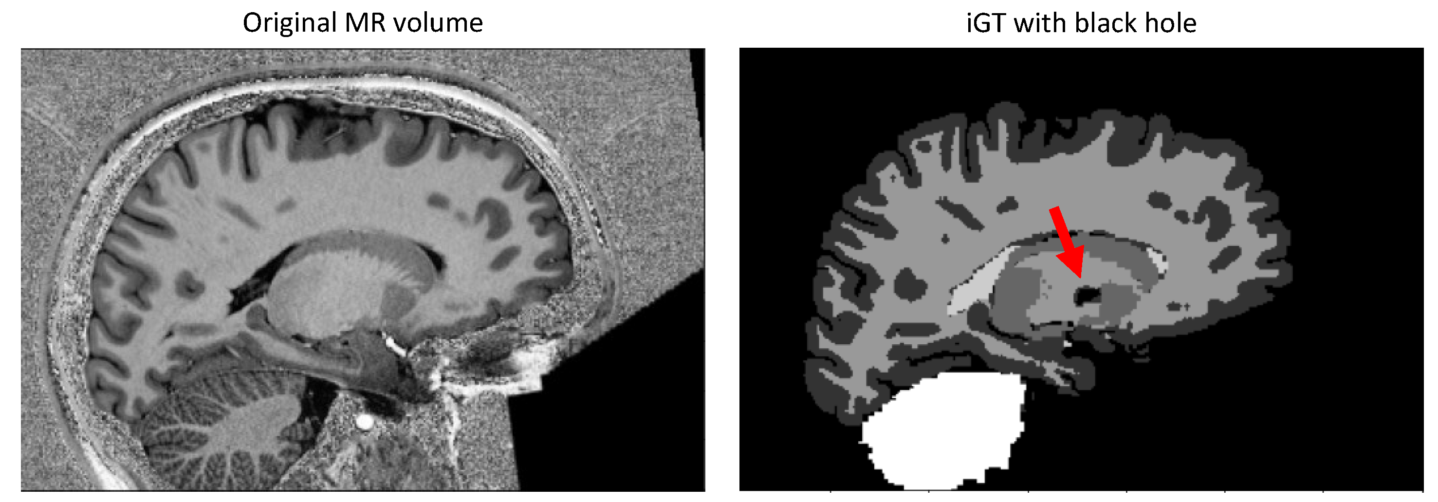
2.1. Data Labeling and Division
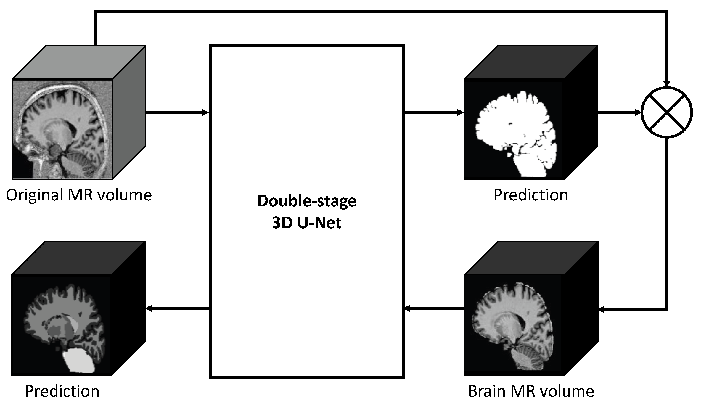
2.2. Double-Stage 3D U-Net
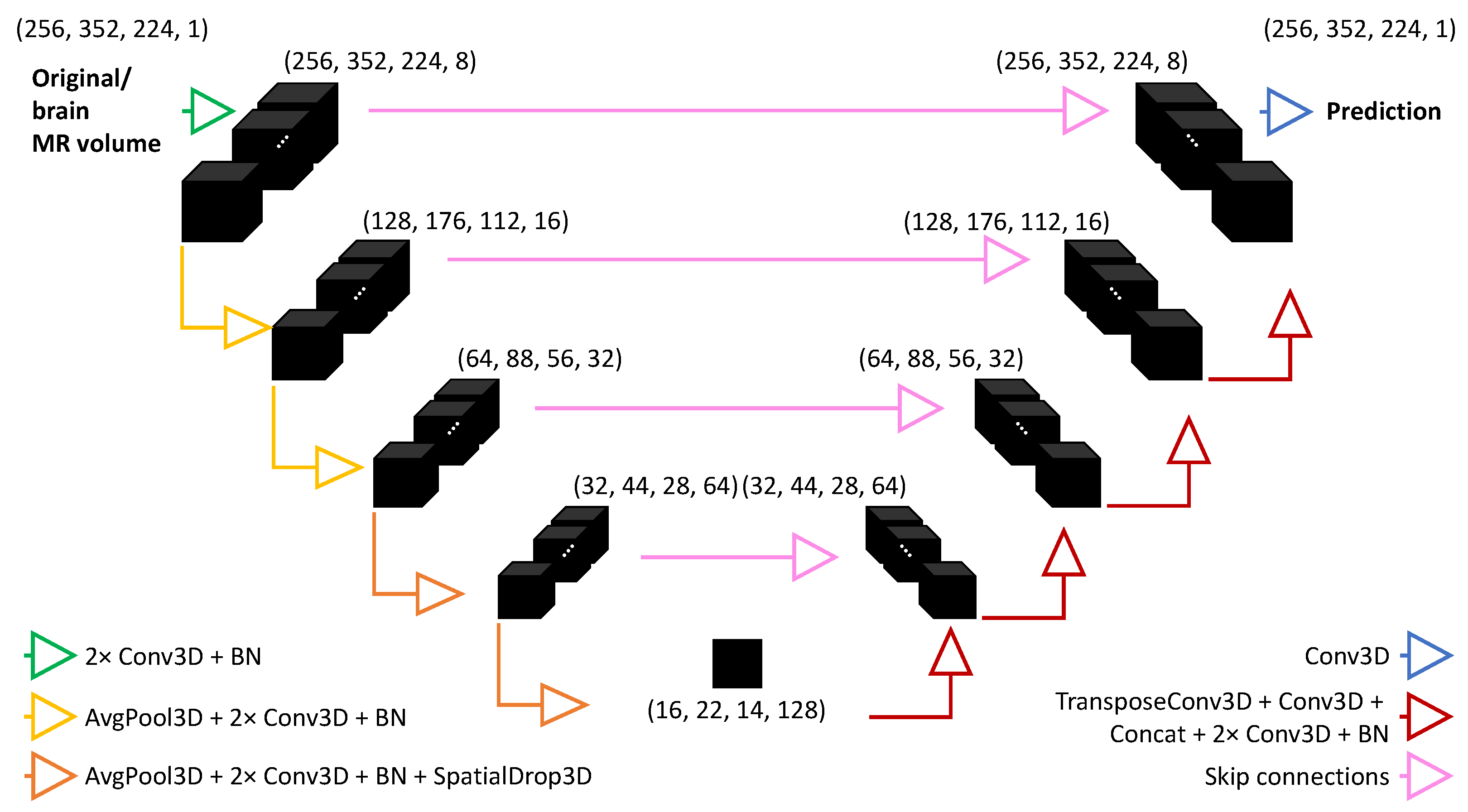
2.2.1. Neural Architecture
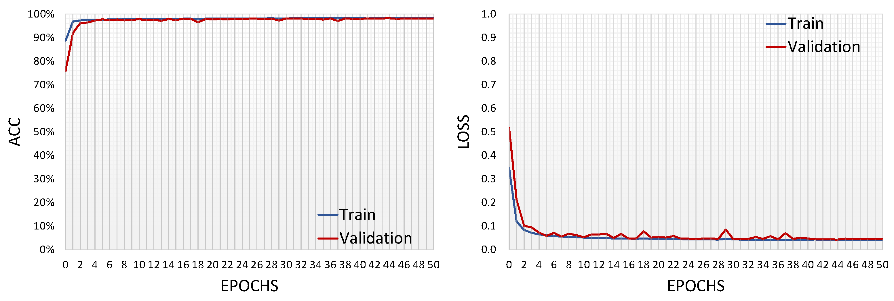
2.2.2. Experimental Setup and Learning Process
2.3. Performance Evaluation and Volume Measure Analysis
3. Results
4. Discussion
5. Conclusions
Author Contributions
Funding
Informed Consent Statement
Data Availability Statement
Acknowledgments
Conflicts of Interest
References
- Haq, E.U.; Huang, J.; Kang, L.; Haq, H.U.; Zhan, T. Image-based state-of-the-art techniques for the identification and classification of brain diseases: A review. Med Biol. Eng. Comput. 2020, 58, 2603–2620. [Google Scholar] [CrossRef] [PubMed]
- Zhao, X.; Zhao, X.M. Deep learning of brain magnetic resonance images: A brief review. Methods 2021, 192, 131–140. [Google Scholar] [CrossRef] [PubMed]
- Tomassini, S.; Sernani, P.; Falcionelli, N.; Dragoni, A.F. CASPAR: Cloud-based Alzheimer’s, schizophrenia and Parkinson’s automatic recognizer. In Proceedings of the IEEE International Conference on Metrology for Extended Reality, Artificial Intelligence and Neural Engineering, Rome, Italy, 26–28 October 2022; pp. 6–10. [Google Scholar]
- Keuken, M.C.; Isaacs, B.R.; Trampel, R.; Van Der Zwaag, W.; Forstmann, B. Visualizing the human subcortex using ultra-high field magnetic resonance imaging. Brain Topogr. 2018, 31, 513–545. [Google Scholar] [CrossRef] [PubMed]
- Helms, G. Segmentation of human brain using structural MRI. Magn. Reson. Mater. Phys. Biol. Med. 2016, 29, 111–124. [Google Scholar] [CrossRef]
- González-Villà, S.; Oliver, A.; Valverde, S.; Wang, L.; Zwiggelaar, R.; Lladó, X. A review on brain structures segmentation in magnetic resonance imaging. Artif. Intell. Med. 2016, 73, 45–69. [Google Scholar] [CrossRef]
- Haque, I.R.I.; Neubert, J. Deep learning approaches to biomedical image segmentation. Inform. Med. Unlocked 2020, 18, 100297. [Google Scholar] [CrossRef]
- Singh, M.K.; Singh, K.K. A review of publicly available automatic brain segmentation methodologies, machine learning models, recent advancements, and their comparison. Ann. Neurosci. 2021, 28, 82–93. [Google Scholar] [CrossRef]
- Despotović, I.; Goossens, B.; Philips, W. MRI segmentation of the human brain: Challenges, methods, and applications. Comput. Math. Methods Med. 2015, 2015, 450341. [Google Scholar] [CrossRef]
- Tomassini, S.; Falcionelli, N.; Sernani, P.; Burattini, L.; Dragoni, A.F. Lung nodule diagnosis and cancer histology classification from computed tomography data by convolutional neural networks: A survey. Comput. Biol. Med. 2022, 146, 105691. [Google Scholar] [CrossRef]
- Fawzi, A.; Achuthan, A.; Belaton, B. Brain image segmentation in recent years: A narrative review. Brain Sci. 2021, 11, 1055. [Google Scholar] [CrossRef]
- Minaee, S.; Boykov, Y.; Porikli, F.; Plaza, A.; Kehtarnavaz, N.; Terzopoulos, D. Image segmentation using deep learning: A survey. IEEE Trans. Pattern Anal. Mach. Intell. 2021, 44, 3523–3542. [Google Scholar] [CrossRef] [PubMed]
- Krithika alias AnbuDevi, M.; Suganthi, K. Review of semantic segmentation of medical images using modified architectures of U-Net. Diagnostics 2022, 12, 3064. [Google Scholar] [CrossRef]
- Sun, L.; Ma, W.; Ding, X.; Huang, Y.; Liang, D.; Paisley, J. A 3D spatially weighted network for segmentation of brain tissue from MRI. IEEE Trans. Med Imaging 2019, 39, 898–909. [Google Scholar] [CrossRef] [PubMed]
- Wang, L.; Xie, C.; Zeng, N. RP-Net: A 3D convolutional neural network for brain segmentation from magnetic resonance imaging. IEEE Access 2019, 7, 39670–39679. [Google Scholar] [CrossRef]
- Bontempi, D.; Benini, S.; Signoroni, A.; Svanera, M.; Muckli, L. CEREBRUM: A fast and fully-volumetric Convolutional Encoder-decodeR for weakly-supervised sEgmentation of BRain strUctures from out-of-the-scanner MRI. Med. Image Anal. 2020, 62, 101688. [Google Scholar] [CrossRef]
- Ramzan, F.; Khan, M.U.G.; Iqbal, S.; Saba, T.; Rehman, A. Volumetric segmentation of brain regions from MRI scans using 3D convolutional neural networks. IEEE Access 2020, 8, 103697–103709. [Google Scholar] [CrossRef]
- Laiton-Bonadiez, C.; Sanchez-Torres, G.; Branch-Bedoya, J. Deep 3D neural network for brain structures segmentation using self-attention modules in MRI images. Sensors 2022, 22, 2559. [Google Scholar] [CrossRef]
- Svanera, M.; Benini, S.; Bontempi, D.; Muckli, L. CEREBRUM-7T: Fast and fully volumetric brain segmentation of 7 Tesla MR volumes. Hum. Brain Mapp. 2021, 42, 5563–5580. [Google Scholar] [CrossRef]
- Cox, R.W. AFNI: Software for analysis and visualization of functional magnetic resonance neuroimages. Comput. Biomed. Res. 1996, 29, 162–173. [Google Scholar] [CrossRef]
- Fracasso, A.; van Veluw, S.J.; Visser, F.; Luijten, P.R.; Spliet, W.; Zwanenburg, J.J.; Dumoulin, S.O.; Petridou, N. Lines of Baillarger in vivo and ex vivo: Myelin contrast across lamina at 7 T MRI and histology. NeuroImage 2016, 133, 163–175. [Google Scholar] [CrossRef]
- Fischl, B. FreeSurfer. NeuroImage 2012, 62, 774–781. [Google Scholar] [CrossRef] [PubMed]
- O’Brien, K.R.; Kober, T.; Hagmann, P.; Maeder, P.; Marques, J.; Lazeyras, F.; Krueger, G.; Roche, A. Robust T1-weighted structural brain imaging and morphometry at 7T using MP2RAGE. PLoS ONE 2014, 9, e99676. [Google Scholar] [CrossRef] [PubMed]
- Yushkevich, P.A.; Piven, J.; Hazlett, H.C.; Smith, R.G.; Ho, S.; Gee, J.C.; Gerig, G. User-guided 3D active contour segmentation of anatomical structures: Significantly improved efficiency and reliability. NeuroImage 2006, 31, 1116–1128. [Google Scholar] [CrossRef]
- Ronneberger, O.; Fischer, P.; Brox, T. U-Net: Convolutional networks for biomedical image segmentation. In Proceedings of the Medical Image Computing and Computer-Assisted Intervention–MICCAI 2015: 18th International Conference, Proceedings, Part III 18, Munich, Germany, 5–9 October 2015; Springer: Berlin/Heidelberg, Germany, 2015; pp. 234–241. [Google Scholar]
- Ioffe, S.; Szegedy, C. Batch normalization: Accelerating deep network training by reducing internal covariate shift. In Proceedings of the International Conference on Machine Learning, Lille, France, 7–9 July 2015; pp. 448–456. [Google Scholar]
- Tomassini, S.; Sbrollini, A.; Covella, G.; Sernani, P.; Falcionelli, N.; Müller, H.; Morettini, M.; Burattini, L.; Dragoni, A.F. Brain-on-Cloud for automatic diagnosis of Alzheimer’s disease from 3D structural magnetic resonance whole-brain scans. Comput. Methods Programs Biomed. 2022, 227, 107191. [Google Scholar] [CrossRef] [PubMed]
- Sugino, T.; Kawase, T.; Onogi, S.; Kin, T.; Saito, N.; Nakajima, Y. Loss weightings for improving imbalanced brain structure segmentation using fully convolutional networks. Healthcare 2021, 9, 938. [Google Scholar] [CrossRef] [PubMed]
- Taha, A.A.; Hanbury, A. Metrics for evaluating 3D medical image segmentation: Analysis, selection, and tool. BMC Med. Imaging 2015, 15, 1–28. [Google Scholar] [CrossRef]
- Le Bihan, D. How MRI makes the brain visible. Make Life Visible; Springer: Singapore, 2020; pp. 201–212. [Google Scholar]
- Ashburner, J.; Barnes, G.; Chen, C.C.; Daunizeau, J.; Flandin, G.; Friston, K.; Kiebel, S.; Kilner, J.; Litvak, V.; Moran, R.; et al. SPM12 Manual; Wellcome Trust Cent. Neuroimaging: London, UK, 2014; Volume 2464. [Google Scholar]
- Jenkinson, M.; Beckmann, C.F.; Behrens, T.E.; Woolrich, M.W.; Smith, S.M. FSL. NeuroImage 2012, 62, 782–790. [Google Scholar] [CrossRef]
- Zhang, F.; Breger, A.; Cho, K.I.K.; Ning, L.; Westin, C.F.; O’Donnell, L.J.; Pasternak, O. Deep learning based segmentation of brain tissue from diffusion MRI. NeuroImage 2021, 233, 117934. [Google Scholar] [CrossRef]
- Kagadis, G.C.; Kloukinas, C.; Moore, K.; Philbin, J.; Papadimitroulas, P.; Alexakos, C.; Nagy, P.G.; Visvikis, D.; Hendee, W.R. Cloud computing in medical imaging. Med. Phys. 2013, 40, 070901. [Google Scholar] [CrossRef]
- Erfannia, L.; Alipour, J. How does cloud computing improve cancer information management? A systematic review. Inform. Med. Unlocked 2022, 33, 101095. [Google Scholar] [CrossRef]


| Layer | Output Shape | Number of Parameters |
|---|---|---|
| Input | (None, 256, 352, 2, 24, 1) | 0 |
| Conv3D | (None, 256, 352, 22, 4, 8) | 224 |
| Conv3D | (None, 256, 352, 22, 4, 8) | 1736 |
| BN | (None, 256, 352, 22, 4, 8) | 32 |
| AvgPool3D | (None, 128, 176, 11, 2, 8) | 0 |
| Conv3D | (None, 128, 176, 11, 2, 16) | 3472 |
| Conv3D | (None, 128, 176, 11, 2, 16) | 6928 |
| BN | (None, 128, 176, 11, 2, 16) | 64 |
| AvgPool3D | (None, 64, 88, 56, 16) | 0 |
| Conv3D | (None, 64, 88, 56, 32) | 13,856 |
| Conv3D | (None, 64, 88, 56, 32) | 27,680 |
| BN | (None, 64, 88, 56, 32) | 128 |
| AvgPool3D | (None, 32, 44, 28, 32) | 0 |
| Conv3D | (None, 32, 44, 28, 64) | 55,360 |
| Conv3D | (None, 32, 44, 28, 64) | 110,656 |
| BN | (None, 32, 44, 28, 64) | 256 |
| SpatialDrop3D | (None, 32, 44, 28, 64) | 0 |
| AvgPool3D | (None, 16, 22, 14, 64) | 0 |
| Conv3D | (None, 16, 22, 14, 128) | 221,312 |
| Conv3D | (None, 16, 22, 14, 128) | 442,496 |
| BN | (None, 16, 22, 14, 128) | 512 |
| SpatialDrop3D | (None, 16, 22, 14, 128) | 0 |
| TransposeConv3D | (None, 32, 44, 28, 64) | 65,600 |
| Conv3D | (None, 32, 44, 28, 64) | 32,832 |
| Concat | (None, 32, 44, 28, 128) | 0 |
| Conv3D | (None, 32, 44, 28, 64) | 221,248 |
| Conv3D | (None, 32, 44, 28, 64) | 110,656 |
| BN | (None, 32, 44, 28, 64) | 256 |
| TransposeConv3D | (None, 64, 88, 56, 32) | 16,416 |
| Conv3D | (None, 64, 88, 56, 32) | 8224 |
| Concat | (None, 64, 88, 56, 64) | 0 |
| Conv3D | (None, 64, 88, 56, 32) | 55,328 |
| Conv3D | (None, 64, 88, 56, 32) | 27,680 |
| BN | (None, 64, 88, 56, 32) | 128 |
| TransposeConv3D | (None, 128, 176, 11, 2, 16) | 4112 |
| Conv3D | (None, 128, 176, 11, 2, 16) | 2064 |
| Concat | (None, 128, 176, 11, 2, 32) | 0 |
| Conv3D | (None, 128, 176, 11, 2, 16) | 13,840 |
| Conv3D | (None, 128, 176, 11, 2, 16) | 6928 |
| BN | (None, 128, 176, 11, 2, 16) | 64 |
| TransposeConv3D | (None, 256, 352, 22, 4, 8) | 1032 |
| Conv3D | (None, 256, 352, 22, 4, 8) | 520 |
| Concat | (None, 256, 352, 22, 4, 16) | 0 |
| Conv3D | (None, 256, 352, 22, 4, 8) | 3464 |
| Conv3D | (None, 256, 352, 22, 4, 8) | 1736 |
| BN | (None, 256, 352, 22, 4, 8) | 32 |
| Conv3D | (None, 256, 352, 22, 4, 2/7) | 18/63 |
| Total: 1,456,890/1,456,935 | ||
| Trainable: 1,456,154/1,456,199 | ||
| Non-trainable: 736 |
| First Learning Stage | Second Learning Stage | ||||
|---|---|---|---|---|---|
| Metrics | Class | Training | Validation | Training | Validation |
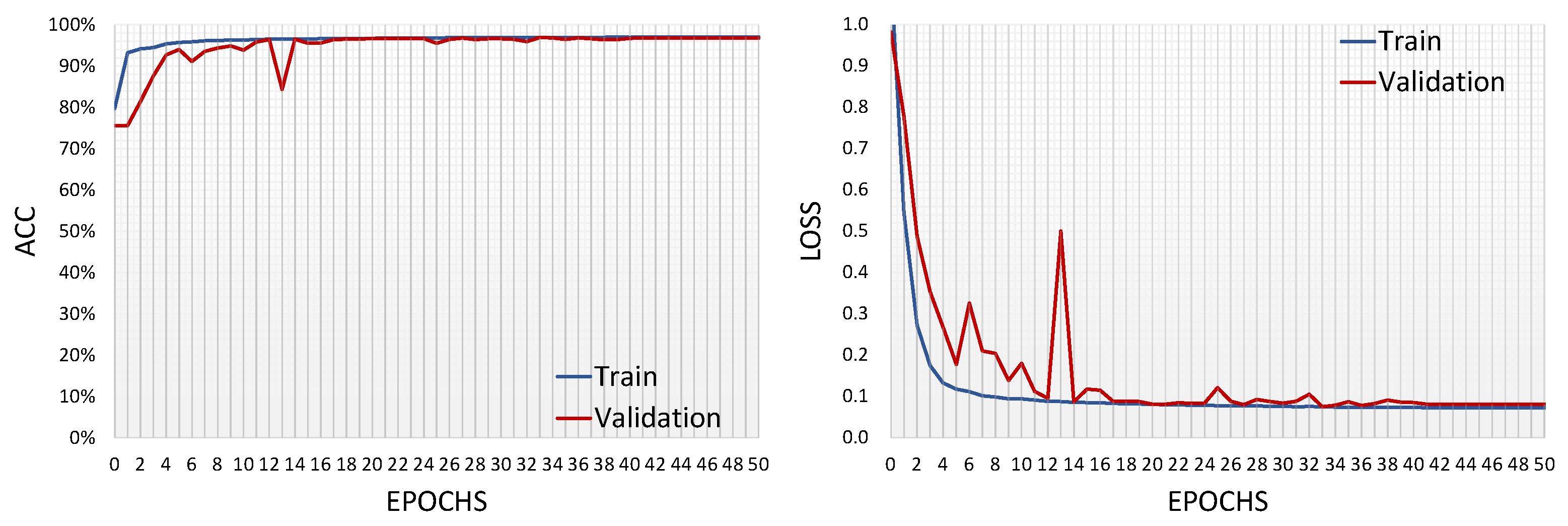
| ACC (%) | All | 98.31 | 98.24 | 96.95 | 96.93 |
| Loss (−) | All | 0.04 | 0.04 | 0.08 | 0.08 |
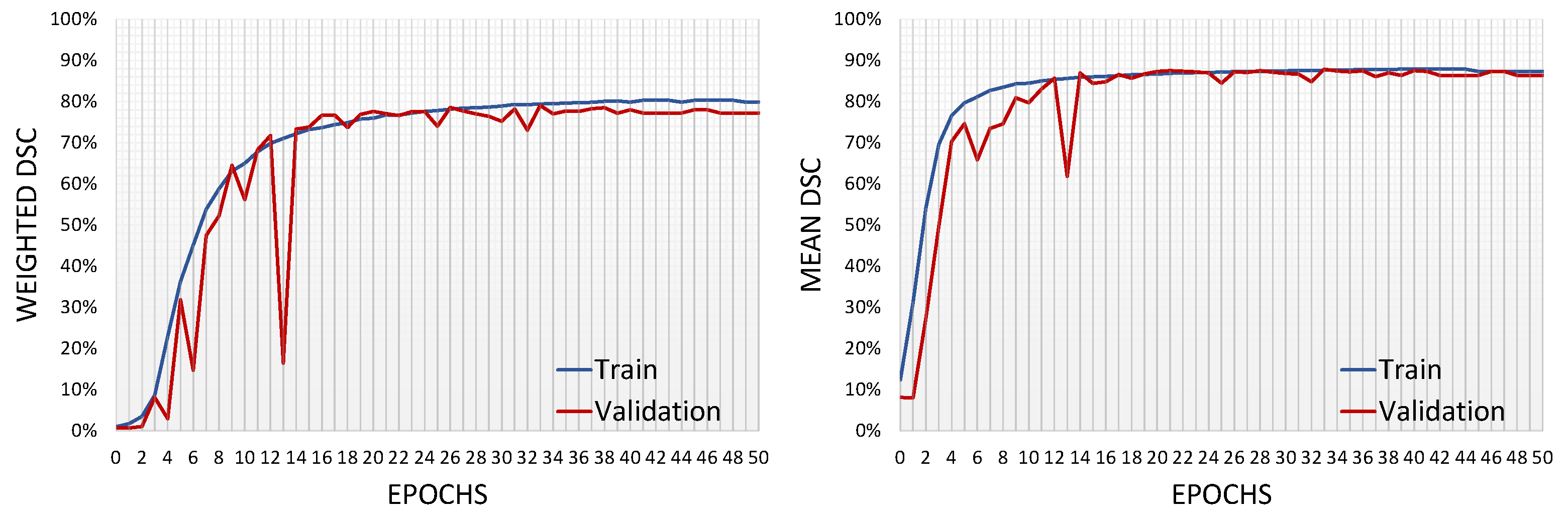
| Weighted DSC (%) | All | - | - | 79.41 | 79.09 |
| Mean DSC (%) | All | - | - | 87.63 | 87.91 |
| DSC (%) | GM | - | - | 86.62 | 87.46 |
| BG | - | - | 80.42 | 80.54 | |
| WM | - | - | 91.46 | 92.53 | |
| VEN | - | - | 82.22 | 82.05 | |
| CB | - | - | 88.81 | 88.48 | |
| BS | - | - | 87.09 | 86.55 | |
| Class | Learning Stage | DSC (%) | VS (%) | HD95 (mm) |
|---|---|---|---|---|
| Background | First | 98.78 ± 0.22 | 99.75 ± 0.25 | 2.74 ± 0.68 |
| Brain | First | 96.33 ± 0.51 | 99.27 ± 0.67 | 3.36 ± 0.54 |
| GM | Second | 90.24 ± 1.04 | 98.61 ± 1.33 | 1.15 ± 0.21 |
| BG | Second | 87.55 ± 0.83 | 94.88 ± 1.82 | 2.94 ± 0.31 |
| WM | Second | 93.82 ± 0.87 | 98.38 ± 1.51 | 1.03 ± 0.11 |
| VEN | Second | 85.77 ± 4.16 | 96.91 ± 2.11 | 2.15 ± 0.94 |
| CB | Second | 91.53 ± 1.96 | 96.87 ± 2.05 | 5.93 ± 1.73 |
| BS | Second | 89.95 ± 2.63 | 97.46 ± 1.36 | 2.92 ± 0.91 |
| Class | Learning Stage | iGT (cm) | Prediction (cm) | MAE (%) |
|---|---|---|---|---|
| Brain | First | 1269 [1152; 1312] | 1253 [1162; 1313] | 1.02 [0.83; 1.73] |
| GM | Second | 624 [581; 663] | 630 [589; 672] | 2.11 [0.55; 3.66] |
| BG | Second | 46 [42; 47] | 50 [48; 54] * | 11.72 [8.69; 14.29] |
| WM | Second | 444 [385; 461] | 421 [386; 446] | 2.45 [1.28; 4.39] |
| VEN | Second | 16 [15; 21] | 16 [15; 21] | 6.56 [0; 8] |
| CB | Second | 109 [104; 115] | 110 [106; 113] | 5.83 [4.27; 10] |
| BS | Second | 17 [16; 18] | 17 [16; 18] | 5.72 [5.26; 7.14] |
Disclaimer/Publisher’s Note: The statements, opinions and data contained in all publications are solely those of the individual author(s) and contributor(s) and not of MDPI and/or the editor(s). MDPI and/or the editor(s) disclaim responsibility for any injury to people or property resulting from any ideas, methods, instructions or products referred to in the content. |
© 2023 by the authors. Licensee MDPI, Basel, Switzerland. This article is an open access article distributed under the terms and conditions of the Creative Commons Attribution (CC BY) license (https://creativecommons.org/licenses/by/4.0/).
Share and Cite
Tomassini, S.; Anbar, H.; Sbrollini, A.; Mortada, M.J.; Burattini, L.; Morettini, M. A Double-Stage 3D U-Net for On-Cloud Brain Extraction and Multi-Structure Segmentation from 7T MR Volumes. Information 2023, 14, 282. https://doi.org/10.3390/info14050282
Tomassini S, Anbar H, Sbrollini A, Mortada MJ, Burattini L, Morettini M. A Double-Stage 3D U-Net for On-Cloud Brain Extraction and Multi-Structure Segmentation from 7T MR Volumes. Information. 2023; 14(5):282. https://doi.org/10.3390/info14050282
Chicago/Turabian StyleTomassini, Selene, Haidar Anbar, Agnese Sbrollini, MHD Jafar Mortada, Laura Burattini, and Micaela Morettini. 2023. "A Double-Stage 3D U-Net for On-Cloud Brain Extraction and Multi-Structure Segmentation from 7T MR Volumes" Information 14, no. 5: 282. https://doi.org/10.3390/info14050282