Article

Energy-Efficient Parallel Computing: Challenges to Scaling

by
Alexey Lastovetsky
and
Ravi Reddy Manumachu
*,†
School of Computer Science, University College Dublin, D04V1W8 Dublin, Ireland
*
Author to whom correspondence should be addressed.
These authors contributed equally to this work.
Information 2023, 14(4), 248; https://doi.org/10.3390/info14040248
Submission received: 13 February 2023 / Revised: 14 April 2023 / Accepted: 18 April 2023 / Published: 20 April 2023
(This article belongs to the Special Issue Advances in High Performance Computing and Scalable Software)

Abstract

:
The energy consumption of Information and Communications Technology (ICT) presents a new grand technological challenge. The two main approaches to tackle the challenge include the development of energy-efficient hardware and software. The development of energy-efficient software employing application-level energy optimization techniques has become an important category owing to the paradigm shift in the composition of digital platforms from single-core processors to heterogeneous platforms integrating multicore CPUs and graphics processing units (GPUs). In this work, we present an overview of application-level bi-objective optimization methods for energy and performance that address two fundamental challenges, non-linearity and heterogeneity, inherent in modern high-performance computing (HPC) platforms. Applying the methods requires energy profiles of the application’s computational kernels executing on the different compute devices of the HPC platform. Therefore, we summarize the research innovations in the three mainstream component-level energy measurement methods and present their accuracy and performance tradeoffs. Finally, scaling the optimization methods for energy and performance is crucial to achieving energy efficiency objectives and meeting quality-of-service requirements in modern HPC platforms and cloud computing infrastructures. We introduce the building blocks needed to achieve this scaling and conclude with the challenges to scaling. Briefly, two significant challenges are described, namely fast optimization methods and accurate component-level energy runtime measurements, especially for components running on accelerators.

1. Introduction

The energy consumption of Information and Communications Technology (ICT) accounted for 7% of the global electricity usage in 2020 and is forecast to be around the average of the best-case and expected scenarios (7% and 21%) by 2030 [1]. This trend makes the energy efficiency of digital platforms a large new technological challenge.
There are two main approaches to responding to this challenge—hardware and software. The first approach deals with energy-efficient hardware devices at a transistor (or gate) level and aims to produce electronic devices consuming as little power as possible.
The second approach deals with the development of energy-efficient software. On the level of solutions, it can be further subdivided into the system-level and applicationlevel approaches. The system-level approach tries to optimize the execution environment rather than the application. It is currently a mainstream approach using Dynamic Voltage and Frequency Scaling (DVFS), Dynamic Power Management (DPM), and energy-aware scheduling to optimize the energy efficiency of the execution of the application. DVFS reduces the dynamic power a processor consumes by throttling its clock frequency. Briefly, dynamic power is consumed due to the switching activity in the processor’s circuits. Static power is consumed when the processor is idle. DPM turns off the electronic components or moves them to a low-power state when idle to reduce energy consumption.
The application-level energy optimization techniques use application-level decision variables and aim to optimize the application rather than the executing environment [2,3]. This category’s most important decision variable is workload distribution.
The development of energy-efficient software employing application-level energy optimization techniques has become an important category owing to the paradigm shift in the composition of digital platforms from single-core processors to heterogeneous platforms integrating multicore CPUs and graphics processing units (GPUs). This paradigm shift has created significant opportunities for application-level energy optimization and bi-objective optimization for energy and performance.
In this work, we present an overview of the application-level bi-objective optimization methods for energy and performance that address two fundamental challenges, nonlinearity and heterogeneity, inherent in modern HPC platforms. Applying the methods requires energy profiles of computational kernels (components) of a hybrid parallel application executing on the different computing devices of the HPC platform. Therefore, we summarize the research innovations in the three mainstream component-level energy measurement methods and present their accuracy and performance trade-offs.
Finally, accelerating and scaling the optimization methods for energy and performance is crucial to achieving energy efficiency objectives and meeting quality-of-service requirements in modern HPC platforms and cloud computing infrastructures. We introduce the building blocks needed to achieve this scaling and conclude with the challenges to scaling. Briefly, two significant challenges are described, namely fast optimization methods and accurate component-level energy runtime measurements, especially for components running on accelerators.
The paper is organized as follows. Section 2 presents the terminology used in energy-efficient computing, including a brief on bi-objective optimization. Section 3 describes the experimental methodology and statistical confidence in experiments used in this work. Section 4 reviews the application-level optimization methods on modern heterogeneous HPC platforms for energy and performance. Section 5 overviews the state-of-the-art energy measurement methods. Section 6 illuminates the building blocks for scaling for energy-efficient parallel computing and highlights the challenges to scaling. Finally, Section 7 provides concluding remarks.

2. Terminology for Energy-Efficient Computing

The static energy consumption during an application execution is the product of the platform’s static power and the execution time of the application. The static power is the idle power of the platform. The dynamic energy consumption during an application execution is the difference between the total energy consumption of the platform and the static energy consumption.

Brief on Bi-Objective Optimization

A bi-objective optimization problem can be mathematically formulated as follows [4,5]:
m i n i m i z e { T ( X ) , E ( X ) } , Subject to X S
where there are two objective functions, T : R k R and E : R k R .
F ( X ) = ( T ( X ) , E ( X ) ) T denotes the vector of objective functions. The decision vectors X = ( x 0 , . . . , x k 1 ) T belong to the (non-empty) feasible region S . S is a subset of the decision variable space R k . Z ( = F ( S ) ) denotes the feasible objective region. It is a subset of the objective space R 2 . The elements of Z are denoted by F ( X ) or z = ( z 1 , z 2 ) T , where z 1 = T ( X ) and z 2 = E ( X ) are objective values.
The objective functions, T and E, are incommensurable. That is, no solution exists that optimizes both objectives simultaneously.
Definition 1.
A decision vector X * S is Pareto-optimal if there does not exist another decision vector X S such that T ( X ) T ( X * ) , E ( X ) E ( X * ) , and either T ( X ) < T ( X * ) or E ( X ) < E ( X * ) or both [4].
An objective vector z * Z is Pareto-optimal if there is not another objective vector z Z such that z 1 z 1 * , z 2 z 2 * , and z j < z j * for at least one index j.
In this work, we focus on single-objective optimization problems for energy and performance and bi-objective optimization problems for dynamic energy and performance and total energy and performance.

3. Experimental Methodology

We present a brief on the methodology of measurement of the execution time and dynamic energy consumption of the hybrid data-parallel applications used in this work.
The hybrid application is composed of several components executed in parallel. There is a one-to-one mapping between the components and computing devices of the hybrid platform. The execution of an accelerator component involves a dedicated CPU core, running the hosting thread, and the accelerator itself, performing the accelerator code. The execution of the accelerator component includes data transfer between the CPU and accelerator memory, computations by the accelerator code, and data transfer between the accelerator memory and CPU. The execution of a CPU component only involves the CPU cores performing the multithreaded CPU code.
The execution time of a component is measured on the CPU side using a CPU processor clock. The measurement step sequence includes querying the processor clock to obtain the start time, executing the component, querying the processor clock to obtain the end time, and calculating the difference between the end and start times to obtain the execution time.
The dynamic energy consumption of a component is also measured on the CPU side using an energy measurement API [6]. First, the total energy consumption of the platform during the component execution is measured. The measurement step sequence includes starting the energy meter, executing the component, stopping the energy meter, and then querying the energy meter for the total energy consumption of the platform. All the steps in the sequence are invoked from the CPU side. The dynamic energy consumption of a component equals the difference between the total energy consumption and the static energy consumption, which is the static power consumption of the platform multiplied by the execution time of the component.

3.1. Precautions to Reduce Noise in Measurements

The hybrid nodes (Figure 1) are fully reserved and dedicated to the experiments during their execution. Several precautions are taken in measuring energy consumption to eliminate any potential interference of the computing elements that are not part of the component running the application kernel.
Energy consumption of a CPU component also includes the contribution from NIC, SSDs, and fans. Therefore, we ensure they are used minimally during the execution of an application to lessen their contribution to dynamic energy consumption. In this way, the contribution of CPUs and DRAM dominates the dynamic energy consumption. The following steps are employed for this purpose:
  • The disk consumption is monitored before and during the application run and ensures no I/O is performed by the application using tools such as sar and iotop.
  • The workload used in the execution of an application does not exceed the main memory, and swapping (paging) does not occur.
  • The application does not use the network by monitoring using tools such as sar and atop.
  • The application kernel’s CPU affinity mask is set using SCHED API’s system call, SCHED_SETAFFINITY().
Fans are significant contributors to energy consumption. On our hybrid nodes, fans are controlled in zones: (a) zone 0: CPU or system fans; (b) zone 1: peripheral zone fans. There are four levels to the control of fan speeds:
  • Standard: Baseboard management controller (BMC) controls both fan zones, with the CPU and peripheral zones set at speed 50%;
  • Optimal: BMC sets the CPU zone at speed 30% and the peripheral zone at 30%;
  • Heavy IO: BMC sets the CPU zone at speed 50% and the Peripheral zone at 75%;
  • Full: All fans run at 100%.
To rule out fans’ contribution to dynamic energy consumption, we set the fans at full speed before launching the experiments. In this way, fans consume the same amount of power, which is included in the static power consumption of the server. Furthermore, we monitored the server’s temperatures and the fans’ speeds with the help of Intelligent Platform Management Interface (IPMI) sensors during the application run and when there is no application run. We found no significant differences in temperature, and the speeds of fans were the same in both scenarios.
Thus, we ensured that the dynamic energy consumption measured reflects the contribution solely by the component executing the given application kernel.

3.2. Statistical Confidence in Our Experiments

For the results shown in this work, a detailed statistical methodology was used to obtain a sample average for a response variable (energy, power, and execution time) from multiple experimental runs to ensure the reliability of the results. The methodology employed Student’s t-test with a 95% confidence interval and precision of 0.05 (5%) for the sample average. In addition, the assumptions in the Student’s t-test of normality and independence of observations were verified using Pearson’s chi-squared test.

4. Application-Level Optimization Methods on Modern Heterogeneous HPC Platforms for Energy and Performance

This section first presents the lack of opportunity for application-level optimization of energy in a linear and homogeneous HPC world. Then, it highlights the challenges posed by non-linearity and heterogeneity inherent in modern HPC platforms to the optimization of applications for the energy and performance on such platforms. Finally, it overviews solutions addressing the challenges.

4.1. Linearity and Homogeneity

In a linear and homogeneous HPC world, there is no room for application-level optimization of energy. The linearity means that both the dynamic energy consumed by a processor and the execution time are linear functions of the size of the executed workload. The homogeneity means that all processors in the system are identical.
The HPC world was linear and homogeneous before the advent of multicore processors and accelerators. To simulate the pre-multicore single-core CPU era, we studied the execution time and dynamic energy consumption profiles of a multi-threaded application executed on a single core of an Intel Haswell multicore CPU, whose specification is shown in Figure 1. The application employs a highly optimized scientific routine, OpenBLAS DGEMM [7], multiplying two square matrices of size n × n . The workload size equals 2 × n 3 . The application employs one thread bound to the core used for executing the application. Therefore, the workload size is executed by one thread.
Figure 2 shows the execution time and dynamic energy profiles of the application. The numactl tool is used to bind the application to one core. The static and dynamic energy consumption during the application execution is obtained using power meters, which is considered the most accurate method of energy measurement [8]. Hereafter, we will refer to this energy measurement approach as the ground-truth method. One can observe that the execution time and dynamic energy profiles are linear functions of workload size.
Now, consider optimizing the application of energy and performance using p such identical linear parallel processors. Mathematically, any workload distribution between identical linear parallel processors will consume the same dynamic energy, and the loadbalanced distribution of the workload will always be optimal for performance and total energy. We provide the theorems and corresponding proofs in Appendix A.

4.2. Impact of Heterogeneity

The assumption of homogeneity was acceptable in the past when HPC platforms were built from identical processors. However, the modern HPC world is increasingly heterogeneous. For example, more than 30% of the Top500 supercomputer list systems are heterogeneous, integrating various CPUs and GPUs [9]. In addition, there is a plethora of research on programming models and tools, benchmark suites, and applications for heterogeneous CPU-GPU compute platforms [10,11,12]. The implications of heterogeneity for bi-objective optimization of applications for performance and energy are profound.
Khaleghzadeh et al. [13] study the bi-objective optimization problem for performance and energy for the simple case of two heterogeneous processors characterized by linear execution time and energy functions. The study reveals an infinite number of globally Pareto-optimal solutions distributing a given workload between the processors. Furthermore, the study found that the only load-balanced solution is Pareto-optimal and will minimize the execution time. The solution using the single most energy-efficient processor will also be Pareto-optimal and minimize dynamic energy consumption.
Figure 3a–c illustrate the results of the study. Figure 3a contains the linear execution time functions of two processors P 1 and P 2 . Figure 3b shows the linear energy functions of the same two processors. The functions were obtained using a well-known and highly optimized matrix multiplication application executing on one core of a multicore CPU. The Pareto front is a linear segment connecting the performance-optimal and energy-optimal endpoints and is shown in Figure 3c. Apart from the performance-optimal solution, all other Pareto-optimal solutions are load-imbalanced.
Motivated by these findings, the authors [14] comprehensively study these implications for the general case of p linear heterogeneous processors executing workload size n. A more general problem is actually solved in this research, allowing performance profiles to be just continuously monotonically increasing, not necessarily linear.
Figure 4 illustrates the p linear heterogeneous processors characterized by p linear increasing time functions, { f 0 , , f p 1 } , in sets F and p linear increasing energy functions, { g 0 , , g p 1 } , in set G. The shape of the Pareto front shown in Figure 4c is found to be a piece-wise continuous linear function consisting of a chain of p 1 linear segments, { S 0 , , S p 2 } , connecting the performance-optimal and energy-optimal endpoints. The other qualitative conclusions apply to the endpoints. The performance-optimal endpoint is the load-balanced solution that distributes the workload in proportion to the speeds of the processors. The energy-optimal endpoint has the total workload assigned to the most energy-efficient processor, the processor with linear energy function with the lowest slope.
Furthermore, the research work [14] proposes efficient exact polynomial algorithms constructing the Pareto front for performance and dynamic energy and performance and total energy. The algorithms exhibit time complexity of O ( p 3 × log 2 n ) . In addition, an exact algorithm is presented that finds the Pareto-optimal solution for a given point in the Pareto front in linear time O ( p ) .
In Appendix B, we illustrate the findings of the study [14] using a highly optimized matrix multiplication application executing on a heterogeneous computing platform shown in Figure 1 comprising five heterogeneous processors ( p = 5 ). The algorithms take input performance and dynamic energy functions that are linear approximations of the profiles. Figure A2 shows the output Pareto fronts for two workloads. Each Pareto front contains p 1 = 4 linear segments. The solution with minimal execution time (shown as a circle) is the load-balancing solution.

4.3. Impact of Non-Linearity

The assumption of linearity was acceptable for single-core processors. However, modern CPUs and accelerators are all multicore, and their performance and energy profiles have proved to be non-linear for popular and carefully optimized applications for such platforms [2].

4.3.1. Multicore CPUs

To illustrate the non-linearity of modern multicore CPUs, we study the performance and energy profiles of two real-life scientific applications executing on the Intel Haswell processor comprising two sockets of 12 cores each (Figure 1). The OpenBLAS DGEMM application [7] multiplies two matrices of size x × n and n × n . The FFTW application [15] computes a 2D fast Fourier transform (FFT) of a dense signal matrix of size n × n . Both applications are multi-threaded and are executed by T threads.
Figure 5 contains the profiles for the OpenBLAS DGEMM application employing 24 threads. Figure 6 contains the profiles for the FFTW application employing 24 threads. The workload size is equally distributed between the threads. The variations in the figures are reproducible owing to the detailed statistical methodology employed in the experiments.
The variations are not due to constant and stochastic fluctuations experienced by a node while executing a workload as an integral part of a common network of computers. Instead, such fluctuations produce variations in the speed that is best represented by a band. The width of the band characterizes the speed variations over time due to load changes [16,17,18]. The width decreases as the workload size increases for uniprocessor (single-core) CPU nodes. However, variations in the presented graph exhibit a different pattern. Therefore, the variations are not caused by random fluctuations in the executing environment. Instead, they are due to the systematic complexity of the integration of resources in multicore processors. Hence, they are an inherent trait of applications executing on multicore servers with resource contention and Non-Uniform Memory Access (NUMA).
Figure 7 graphs the variations for the OpenBLAS DGEMM application as the number of threads executing in the application increases. The fluctuations increase with the number of threads and reach the peak for 24 threads, which equals the total number of physical cores in the server. The figure shows that the variations are noticeable even for a smaller number of threads ( T = 2 ).
Furthermore, Figure 6 illustrates the large magnitude of the variations exhibiting performance drops of around 70% for many workload sizes (in the speed function plot).
This behavior for performance and energy implies that the discrete non-linear functions of the execution time and energy consumption against the workload size are highly irregular and impossible to be approximated by smooth functions.
In addition, the variations in execution time and energy consumption are often not correlated. Namely, the increase in workload can lead to a decrease in execution time and an increase in energy consumption or to an increase in execution time and a decrease in energy consumption. Therefore, the lack of correlation presents a significant opportunity for bi-objective optimization for performance and energy.
To further explore the potential trade-offs between performance and dynamic energy, we look at the improvements in performance obtained when using workload distribution, minimizing the dynamic energy consumption and the improvements in energy obtained when using workload distribution, maximizing performance for the OpenBLAS DGEMM and FFTW applications.
Optimizing for performance alone can lead to a sound reduction in dynamic energy consumption. For OpenBLAS DGEMM, the average and maximum percentage reductions in energy were 12% and 68%, respectively. For FFTW, the average and maximum percentage reductions in energy were 23% and 55%, respectively. However, optimizing for energy alone can cause significant performance degradation. For OpenBLAS DGEMM, the average and maximum performance degradations were 95% and 100%. For FFTW, the average and maximum performance degradations were close to 100% and 100%, respectively.

4.3.2. Graphics Processing Units (GPUs)

Khaleghzadeh et al. [13] studied the execution time and dynamic energy profiles of a matrix multiplication application and a 2D FFT application on two Nvidia GPUs. They show that the GPUs also exhibit drastic variations similar to the multicore CPUs. We present the findings for the 2D-FFT application here.
Figure 8 shows the execution time and dynamic energy profiles of the 2D-FFT application. The application computes a 2D discrete Fourier Transform of a complex signal matrix of size n × n . The workload size is 5.0 × n 2 × log 2 n . It employs CUFFT routines. The same detailed statistical methodology is followed to ensure the reliability of the results. The dynamic energy consumption is obtained using the ground-truth method. CUFFT routines give failures for n that cannot be factored into primes less than or equal to 127. For these matrix sizes, we find a matrix size n l greater than n for which CUFFT provides a solution. Therefore, we pad the input matrix to increase its problem size from n to n l and zero the contents of the extra padded areas. For problem sizes ( n 2 ) exceeding the main memory of the GPU, out-of-core computations are employed.
Figure 9 shows the zoomed plot of the dynamic energy profile. One can see that the execution time and dynamic energy profiles are highly non-linear. Furthermore, we find that the variations in execution time and energy consumption are not correlated.
Therefore, there is a need for novel methods of solving optimization problems on modern HPC platforms for energy and performance that consider the non-linearity and heterogeneity inherent in such platforms. We now review research in this direction.

4.4. Optimization Methods for Energy and Performance on Modern HPC Platforms

This section overviews solutions addressing the challenges posed by non-linearity and heterogeneity inherent in modern HPC platforms to the optimization of applications for energy and performance on such platforms.

4.4.1. Non-Linearity on Homogeneous Platforms

Lastovetsky et al. [2] study the implications of the non-linearity of homogeneous multiprocessors for optimizing applications for performance or energy. They formulate the single-objective optimization problems of data-parallel applications for performance and energy on homogeneous clusters of multicore CPUs. They propose data partitioning algorithms solving the problems that take as input application-specific performance and dynamic energy profiles of the multicore CPU processor. The profiles are discrete functions of workload size of arbitrary shape. They realistically consider the resource contention and NUMA inherent in modern multicore CPU platforms. The algorithms output performance-optimal and energy-optimal workload distributions and exhibit the time complexity of O ( p 2 ) where p is the number of homogeneous processors. The performance-optimal and energy-optimal solutions are not necessarily load-balanced.
Motivated by the findings in [2], Reddy et al. [3] study the bi-objective optimization of data-parallel applications on homogeneous multicore CPU clusters for performance and energy. The problem has workload distribution as the only decision variable. The authors propose an exact global optimization algorithm solving the problem exhibiting time complexity of O ( m 2 × p 2 ) , where m is the cardinality of discrete performance and energy profiles and p is the number of homogeneous processors. The algorithm takes discrete performance and dynamic energy functions against workload size as input and outputs the globally Pareto-optimal set of solutions.
The research work [3] experiments with two highly optimized scientific data-parallel applications, OpenBLAS DGEMM [7] and FFTW [15], executed on the Intel Haswell multicore CPU platform (Figure 1). Figure 10 presents a representative sample of the results for two ( n , p ) combinations for both applications where n is the workload size and p is the number of homogeneous processors. For the OpenBLAS DGEMM application, the ( n , p ) combinations are (1024, 9) and (690, 36), and for the FFTW application, (5000, 9) and (4672, 16). The Pareto front output by the exact global optimization algorithm is shown in each figure, along with the load-balanced solution.
The experiments demonstrate that load-balanced solutions, equally distributing the workload between the homogeneous processors and only considered by the state of the art as optimal, are neither performance-optimal nor energy-optimal, and always far away from the Pareto front of globally optimal solutions. The shape of the Pareto front for both applications suggests that significant reductions in energy consumption over the performance-optimal solution can be achieved at the expense of minor increases in execution time. Similarly, significant improvements in performance over the energy-optimal solution can be achieved at the expense of minor increases in energy consumption. Furthermore, the number of globally Pareto-optimal solutions found by the algorithm was significant, providing a wide range of optimal solutions to pick from.

4.4.2. Non-Linearity on Heterogeneous Platforms

Khaleghzadeh et al. [19] propose a novel data-partitioning algorithm (HPOPTA) that solves the single-objective optimization problems of data-parallel applications for performance on p non-linear heterogeneous processors. The algorithm finds the performanceoptimal solution (workload distribution) for the most general shapes of performance profiles for data-parallel applications executing on such platforms. Moreover, it exhibits a time complexity of O ( m 3 × p 3 ) , where m represents the cardinality of the discrete performance functions. Furthermore, the authors propose data-partitioning algorithms in [20] that solve the single-objective optimization problems of data-parallel applications for dynamic or total energy on p non-linear heterogeneous processors. The algorithms find dynamic energy-optimal and total energy-optimal solutions (workload distributions) for the most general shapes of dynamic energy and total energy profiles for data-parallel applications executing on such platforms.
Khaleghzadeh et al. [13] study the bi-objective optimization problem of data-parallel applications for performance and energy on heterogeneous processors. They propose a solution method (HEPOPTA) comprising an efficient and exact global optimization algorithm. The algorithm takes input performance and dynamic energy profiles of the processors as arbitrary discrete functions of workload size and returns the Pareto-optimal solutions (generally load-imbalanced). It has time complexity O ( m 3 × p 3 × log 2 ( m × p ) ) where m is the maximum cardinality of the discrete sets representing the performance and energy profiles of the h heterogeneous processors. Furthermore, the input dynamic energy profiles are obtained using a methodology [21] that accurately models component-level energy consumption of a hybrid data-parallel application using the ground truth method. The number of globally Pareto-optimal solutions for performance and energy found by these algorithms was significant for real-life performance and energy profiles.
In order to apply the energy-optimization methods [2,3,13,14,19,20], we need energy profiles of individual components of a hybrid parallel application and their performance profiles (for bi-objective optimization). Therefore, we need methods for component-level measurement of the execution time and energy.
While the component-level measurement of execution time may not be trivial for tightly coupled units, it is doable as all processing units are equipped with sufficiently precise clocks. However, methods for the component-level measurement of energy consumption represent a real challenge. In the absence of such methods, the problem of building energy profiles of individual components of a hybrid parallel application becomes intractable. Indeed, in this case, we could only use system-level energy measurements. Therefore for a system integrating p heterogeneous processors, we would have to experimentally build the energy profile of cardinality m p (for all possible combinations of workload distribution) instead of m × p (p individual profiles that can be used to calculate energy consumption for all possible combinations of workload distribution given each profile consists of m data points). We now review research progress on component-level measurement of energy consumption.

5. State-of-the-Art Energy Measurement Methods

There are three mainstream energy measurement methods that can be employed for determining component-level energy consumption. The first method is system-level physical power measurements using external power meters. The second method is power measurements provided by on-chip power sensors embedded in mainstream server processors. The third method is energy-predictive models employing measurable runtime performance-related predictor variables.

5.1. System-Level Physical Power Measurements Using External Power Meters

This approach is the most accurate but very expensive. In our experience, it can take hours and even days to obtain a single experimental point with sufficient statistical confidence. The measurements obtained this way are considered ground truth [8].

5.2. On-Chip Power Sensors

Mainstream CPU and GPU processors now provide on-chip power sensors that give power measurements at a high sampling frequency. The measurements can be collected using special programmatic interfaces.
Intel and AMD are the leading vendors for multicore CPU microprocessors with x86-64 architecture. Intel’s brand of Xeon multicore microprocessors competes with AMD’s line of Eypc multicore microprocessors in the HPC server market. Intel’s multicore CPU processors are equipped with a Running Average Power Limit (RAPL) [22] feature that provides power measurements obtained using programmatic and command-line interfaces of Likwid tool [23]. AMD provides the uProf tool [24], which can be used for energy profiling of applications. Nvidia and AMD are the leading vendors of GPUs employed in the HPC server and data center market. Nvidia’s Ampere architecture GPUs compete with AMD’s Instinct GPUs with Compute DNA for the Data Center (CNDA) architecture.

5.2.1. Intel Running Average Power Limit (RAPL)

Intel multicore CPUs offer Running Average Power Limit (RAPL) [22] capability to monitor power and control frequency (and voltage). In addition, RAPL provides energy counters for CPU and DRAM that are further detailed in Appendix C.
Fahad et al. [8] demonstrate that using Intel RAPL in energy optimization may lead to significant energy losses. Experiments with a DGEMM matrix-multiplication hybrid application have shown that using RAPL for building energy profiles for energy optimization methods results in energy losses ranging from 37% to 84% (depending on matrix sizes) in comparison with the use of accurate ground-truth profiles. Appendix C presents the application and experimental results in detail.

5.2.2. AMD Application Power Management (APM)

AMD processors provide average power estimates through the Application Power Management (APM) [25] interface. However, research work [26] reports that APM provides highly inaccurate data, particularly during the processor sleep states.

5.2.3. Intel Manycore Platform Software Stack (Intel MPSS)

Intel Xeon Phi co-processors host an on-board Intel System Management Controller chip (SMC) [27]. It provides energy consumption that is programmatically obtained using the Intel manycore platform software stack (Intel MPSS) [28]. However, there is no record of the accuracy of Intel MPSS in the literature or Intel manuals. Furthermore, these coprocessors have been discontinued.
Fahad et al. [8] examine the accuracy of MPSS for two highly optimized applications, DGEMM and 2D FFT. The DGEMM application multiplies two square matrices of size N × N using the Intel MKL DGEMM routine. The 2D FFT application computes the 2D discrete Fourier transform of a signal matrix of size N × N using the Intel MKL FFT routine. The Intel Xeon Phi processor employed for the experiments is shown in Figure 1. The authors compare the dynamic energy profiles of the applications obtained using MPSS with ground-truth profiles.
The average and maximum errors of MPSS are found to be 40.68% and 55.78%, respectively. Appendix D presents further details on the results.

5.2.4. Nvidia Management Library (NVML)

Nvidia GPUs have on-chip power sensors providing readings that can be obtained programmatically using the Nvidia Management Library (NVML) [29] interface. The reported accuracy of the energy readings in the NVML manual is 5%.
However, Fahad et al. [8] study the accuracy of NVML for two highly optimized applications, CUBLAS DGEMM and CUBLAS FFT, computing the matrix multiplication of two square matrices of size N × N and 2D discrete Fourier transform of a signal matrix of size N × N . The Nvidia GPU employed for the experiments is Nvidia K40c GPU shown in Figure 1. The authors compare the dynamic energy profiles of the applications obtained using NVML with the ground-truth profiles.
The average and maximum errors of NVML are found to be 10.62% and 35.32% for the DGEMM application and 12.45% and 57.77% for the FFT application. Appendix E contains further details on NVML accuracy on Nvidia P100 PCIe GPU.

5.2.5. Summary

While cheap and efficient, on-chip power sensors have been found to be inaccurate and poorly documented. Extensive and solid experiments with several mainstream CPUs, accelerators, and highly optimized scientific kernels have shown that energy profiles constructed using state-of-the-art on-chip power sensors are qualitatively inaccurate. For example, the shape of a dynamic energy profile determined using on-chip sensors differs significantly from the shape obtained with the ground truth, showing the increase in energy consumption in situations where the ground-truth system-level measurements give a decrease and vice versa. Therefore, the energy measurements using on-chip sensors do not capture the holistic picture of the dynamic energy consumption during application execution.

5.3. Software Energy Predictive Models

The third approach uses software energy-predictive models employing various measurable runtime performance-related predictor variables. State-of-the-art models still need to be more accurate but are improving. Nevertheless, this approach is the only realistic alternative to methods using power meters.
Most popular and studied models use Performance Monitoring Counters (PMCs) as predictor variables. PMCs are special-purpose hardware registers provided in modern processor architectures for low-level performance analysis and tuning. However, they are large in number. For example, the Likwid tool [23] offers 1665 architecture events and 143 counters to store the events for the Intel Haswell multicore processor (Figure 1). Out of the 1665 events, there are 164 core-level general-purpose counters, called PMCs. An application must be executed 41 times to collect all the PMCs since only four counters are provided to store the event values. If one includes the cost of statistical averaging to obtain the mean and variance for each event, then collecting all the PMCs and other architecture events becomes prohibitive and practically infeasible at runtime.
For the Intel Skylake multicore processor (Figure 1), Likwid offers 1993 performance events and 329 counters. Therefore, the number of events increases with each new processor generation. Furthermore, the events are architecture-specific and, therefore, non-portable.
Linear PMC-based dynamic energy-predictive models are the most common. Dominant PMC groups for these models include cache misses, branch instructions, floating point operations, page faults, and memory accesses. The issues with PMC-based models are the large number of PMCs to consider, the tremendous programming effort and time to collect PMCs, and the need for portability.
Before 2017, techniques to select PMCs for a model either considered all PMCs to capture all possible contributors to energy consumption, were based on a statistical methodology such as correlation and Principal Component Analysis (PCA), or used expert advice or intuition to pick a subset.
Numerous PMC-based models have been proposed proposed, but none was sufficiently accurate [30]. Although research on energy predictive models reports excellent accuracy, they typically report the prediction accuracy of total energy with a very high static power base. In addition, most reported results surveyed in [30] were not reproducible. The best verifiable average prediction error of average dynamic power by such models for an Intel Haswell multicore CPU (Figure 1) used to validate these models was in the range of 90–100%.

5.3.1. Additivity of Performance Monitoring Counters

One cause of inaccuracy of PMC-based energy models discovered in 2017 is that many popular PMCs are not additive on modern multicore processors [31]. Energy is additive. Indeed, the energy consumption of serial execution of two applications A and B will be equal to the sum of their individual consumptions, E A B = E A + E B . Therefore, any PMC parameter x in a linear power/energy predictive model should be additive, i.e., x A B = x A + x B .
The details of how to obtain the additivity error of a PMC are presented in Appendix F. While all PMCs are additive by description, PMCs that are most commonly used in state-of-the-art energy models are non-additive in practice, some exhibiting up to 200% deviation from additivity [31]. Numbers of non-additive PMCs increase with the increase in cores (very few non-additive PMCs in the case of single core) [31].

5.3.2. Selection of Model Variables Based on Energy Conservation Laws

Another cause of inaccuracy is the violation of basic laws of energy conservation in these models, including non-zero intercepts in dynamic energy models, negative coefficients in additive terms, and non-linearity of some advanced models (including ML models) [31,32].
To understand the practical implications of the basic energy conservation laws for the accuracy of linear energy-predictive models, we present a digest of the theory of energy-predictive models of computing in Appendix G. Briefly, the theory formalizes properties of PMC-based energy predictive models derived from the fundamental physical law of energy conservation. Then, it provides practical implications, including selection criteria for model variables, model intercept, and model coefficients to construct accurate and reliable linear energy predictive models.
Thus, the accuracy of PMC-based dynamic energy models can be improved by removing non-additive PMCs from models and enforcing basic energy conservation laws. Applying this technique has significantly improved the accuracy of state-of-the-art models, bringing it to 25–30% [33,34].

5.3.3. Best Linear Energy Predictive Models for Intel Multicore CPUs

While the theory of energy-predictive models of computing is proposed with PMC-based energy predictive models as the focal point, it can be applied creatively for model variables (such as resource utilization) that account for energy-consuming activities.
Shahid et al. [34] consider models employing processor and memory utilizations and PMCs as model variables. Appendix H presents the mathematical form of the linear models. The model variables are positive and highly additive to meet the requirements of the theory for better model prediction accuracy.
The best models employing Likwid PMCs and utilization variables achieved 10–20% accuracy on popular scientific kernels [34]. Therefore, while there is still a long way to go, the recent results are promising.

5.3.4. Runtime Energy Modeling on Nvidia GPU Accelerators

The CUDA Profiling Tools Interface (CUPTI) [35] tool provides performance events and metrics for Nvidia k40 GPU and Nvidia P100 PCIe GPU (specifications in Figure 1) that are typically employed for performance profiling. Like the PMCs for multicore CPUs, however, they have also been used in dynamic energy predictive models [36,37,38]. For the Nvidia A40 GPU (Table 1), the Nsight Compute profiler is used to obtain the metrics. However, they are quite large in number.
Based on our experiments on these GPUs, many key events and metrics overflow for large matrix sizes ( N > 2048 ) due to 32-bit integers being dedicated to storing the values. Hence, they are unsuitable for the energy-predictive modelling of HPC applications where the problem sizes can be large. However, this problem is not present in Nvidia A40 GPU (Table 1).
There is no equivalent to CPU utilization for Nvidia GPUs. A proxy for utilization, achieved_occupancy, is commonly employed for modeling GPU energy consumption [39,40,41,42]. However, we observed that achieved_occupancy exhibits a complex non-linear non-functional relationship with energy consumption for the data-parallel applications employed in our experiments. Figure 11 shows the relationship between average dynamic power versus achieved_occupancy and performance versus achieved_occupancy for the matrix multiplication application employing the CUBLAS DGEMM routine on Nvidia P100 PCIe GPU. Each data point in the graph is obtained using a rigorous experimental statistical methodology where the application is run repeatedly until the sample mean lies in the 95% confidence interval and a precision of 0.025 (2.5%) is achieved.
There is no method currently available to implement the additivity test for GPUs to determine the most additive model variables. Therefore, selecting reliable model variables based on energy conservation laws for designing accurate software predictive models for accelerators is currently an open research problem.

5.4. Accuracy vs. Performance of Component-Level Energy Measurement Methods

We conclude our overview of energy measurement methods by summarizing their accuracy and performance trade-offs.
Figure 12 summarizes the trade-offs between the accuracy and the performance of the construction of dynamic energy profiles associated with the three energy measurement methods. The best accuracy obtained using the ground truth is equal to the sum of the statistical accuracy of experiments (typically ± 5 % ) and the inherent accuracy of the power meters ( ± 3 % for WattsUp Pro power meters). However, while the ground-truth method has the highest accuracy (8%), it has the lowest performance. On the other hand, the method based on on-chip power sensors has the ideal performance but exhibits the highest inaccuracy (73%), as presented earlier. Moreover, the dynamic energy profile built using this method has a shape that deviates significantly from the ground truth. The method based on energy-predictive models exhibits a good trade-off between these two extremes. If we exclude the cost of construction of the energy-predictive models, it has an ideal performance equivalent to the method based on on-chip sensors since both methods predict the energy consumption using model variables stored in registers. On the other hand, the method based on energy predictive models has an accuracy (11%) close to the ideal. In addition, the dynamic energy profile built using this method has a shape that follows the ground truth.
Therefore, the approach using software energy-predictive models employing various measurable runtime performance-related predictor variables is the only realistic alternative to methods using power meters. Furthermore, this approach is ideally suited to implement software energy sensors, an essential building block for scaling optimization methods for energy and performance that are presented below.

6. Building Blocks for Scaling for Energy-Efficient Parallel Computing

Accelerating and scaling the optimization methods for energy and performance is crucial to achieving energy efficiency objectives and meeting quality-of-service requirements in modern HPC platforms and cloud computing infrastructures.
To elucidate the building blocks needed to achieve this scaling, we will recapitulate the main steps of the optimization methods [2,3,13,14,19,20].
The first step involves modeling the hybrid application if the execution environment is a heterogeneous hybrid platform comprising different computing devices (multicore CPUs and accelerators). A hybrid application comprises several multithreaded kernels executing simultaneously on different computing devices of the platform. The load of one kernel may significantly affect others’ performance due to severe resource contention arising from tight integration. Due to this, modeling each kernel’s performance and energy consumption individually in hybrid applications becomes a problematic task [43].
Therefore, the research above considers hybrid application configurations comprising no more than one kernel per device. Each group of cores executing a kernel is modeled as an abstract processor. Hence, the executing platform is represented by a set of heterogeneous abstract processors. The grouping aims to minimize the contention and mutual dependence between abstract processors. In addition, the sharing of system resources is maximized within groups and minimized between the groups.
Hence, a hybrid application is represented by a set of computational kernels executing on groups of cores, which we term 
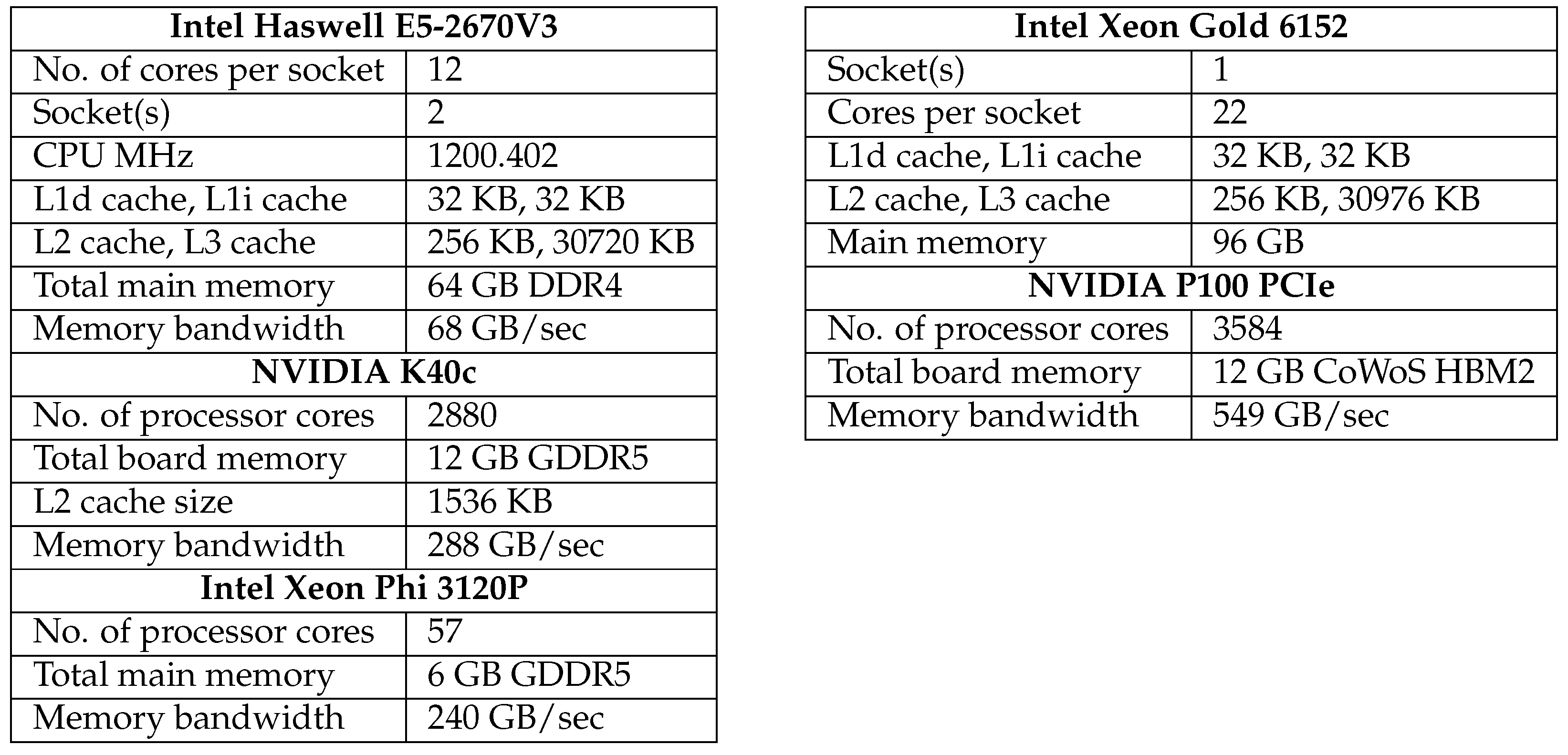
heterogeneous abstract processors. Consider the platform shown in 
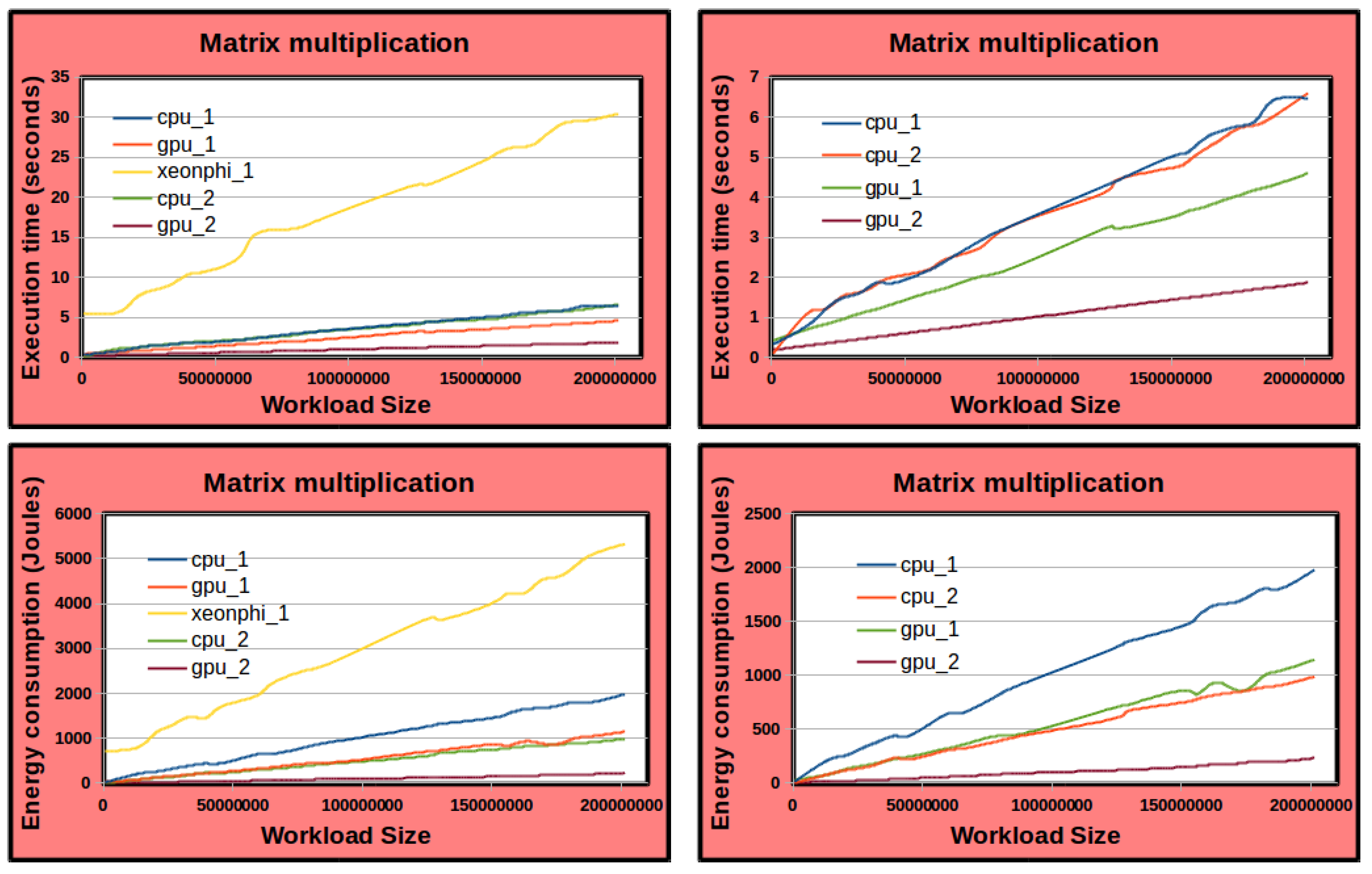
Figure 1 as an example. It consists of two multicore CPUs: a dual-socket Intel Haswell multicore CPU with 24 physical cores with 64 GB main memory and a singlesocket Intel Skylake processor containing 22 cores. The first multicore CPU hosts two accelerators, an Nvidia K40c GPU and an Intel Xeon Phi 3120P. The second multicore CPU hosts an Nvidia P100 PCIe GPU. Therefore, the hybrid application executing on this platform is modeled by four heterogeneous abstract processors, CPU_1, GPU_1, PHI_1, and GPU_2. CPU_1 comprises 22 (out of a total of 24) CPU cores. GPU_1 symbolizes the Nvidia K40c GPU and a host CPU core connected to this GPU via a dedicated PCI-E link. PHI_1 symbolizes the Intel Xeon Phi and a host CPU core connected to this Xeon Phi processor via a dedicated PCI-E link. The Nvidia P100 PCIe GPU and a host CPU core connected to this GPU via a dedicated PCI-E link are denoted by GPU_2.
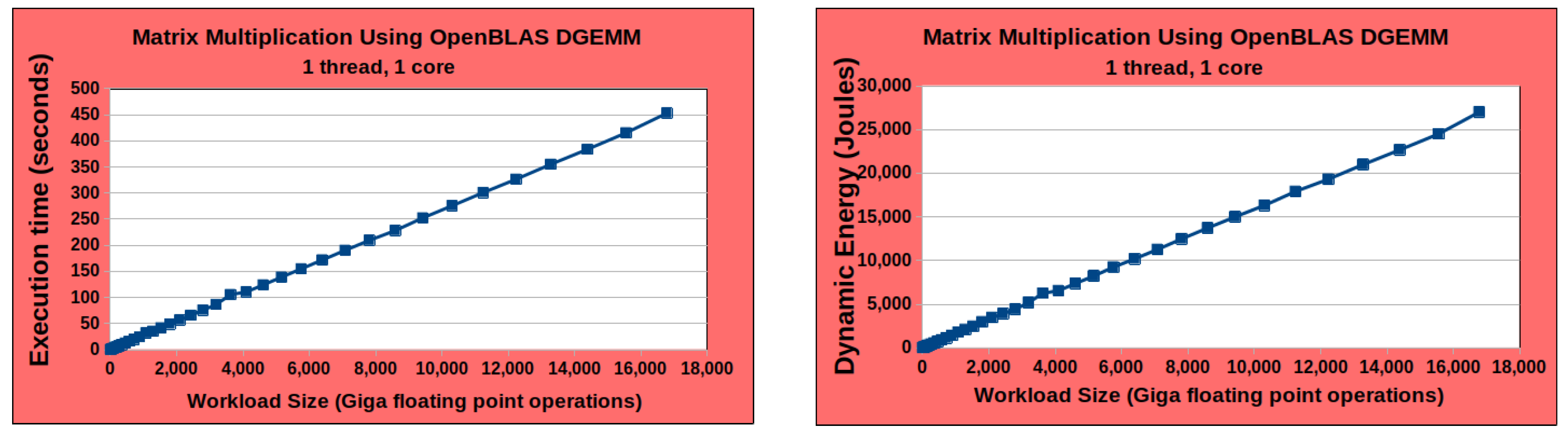
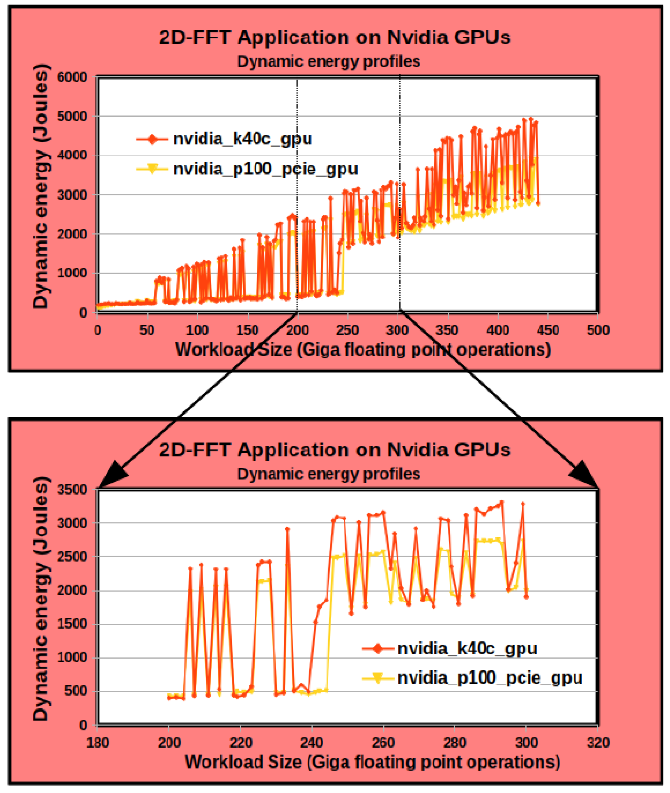
Then, the computational kernels’ performance and dynamic energy profiles are built offline using a methodology based on processor clocks and system-level power measurements provided by external power meters (ground-truth method).
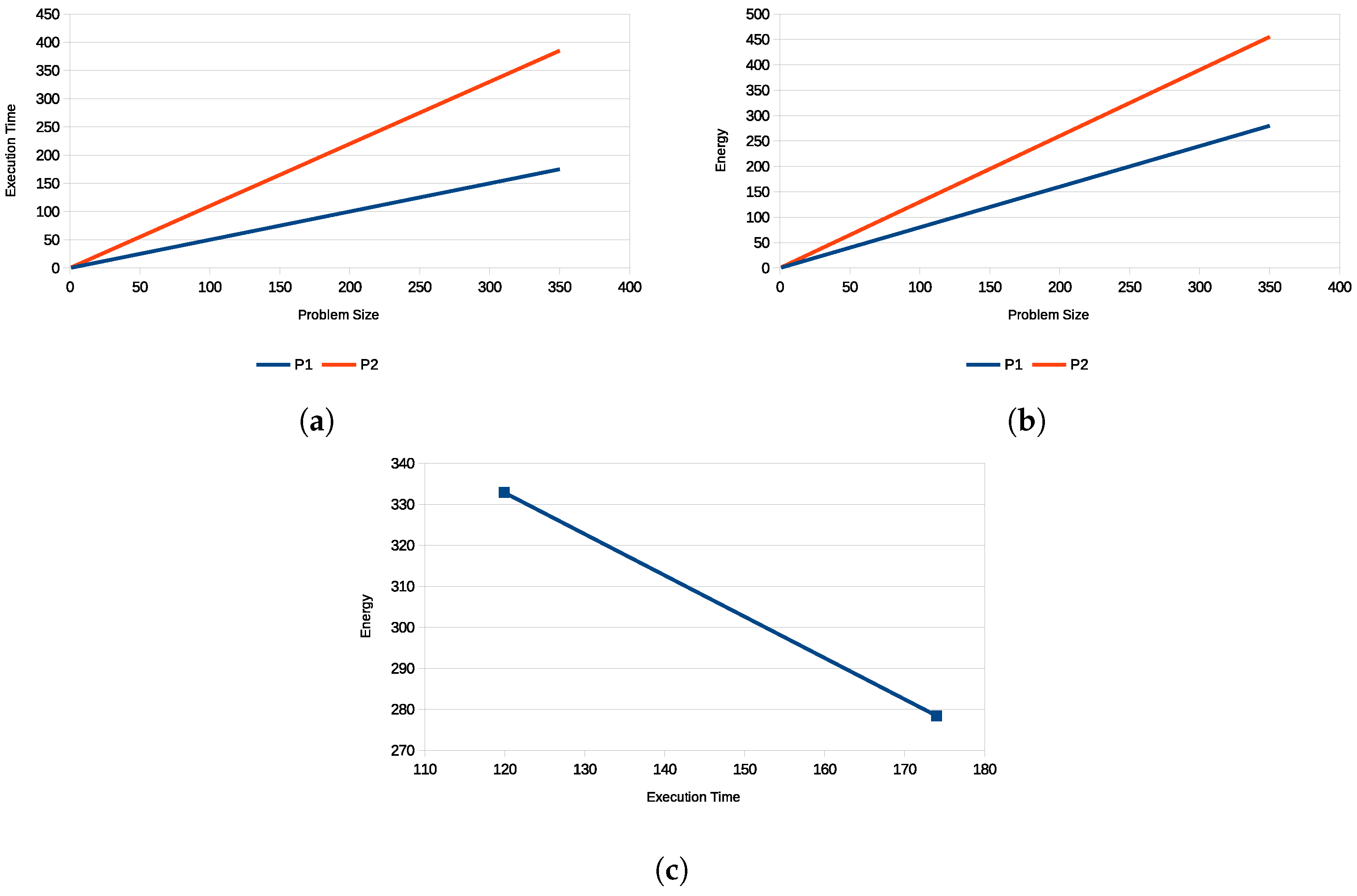
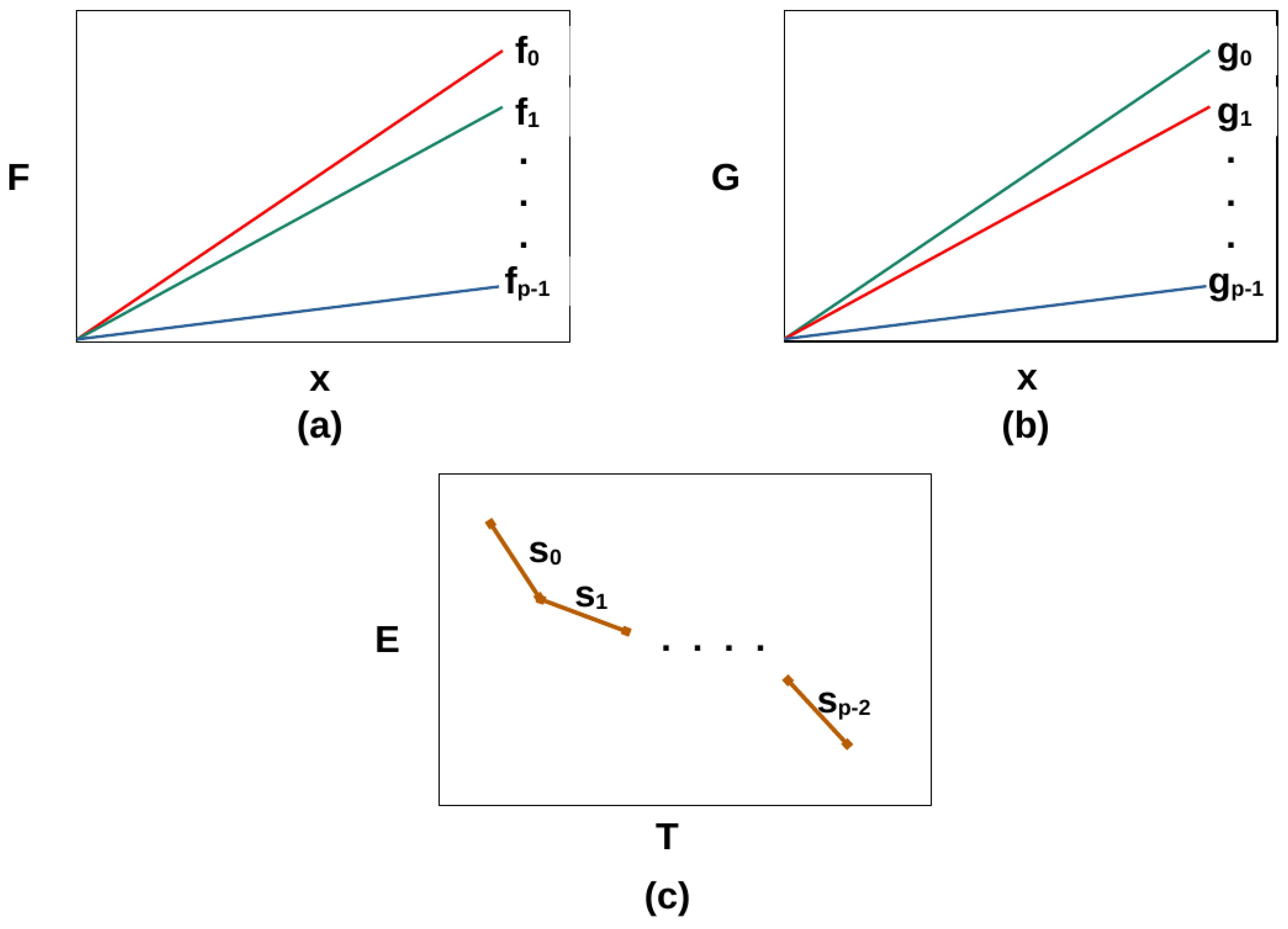
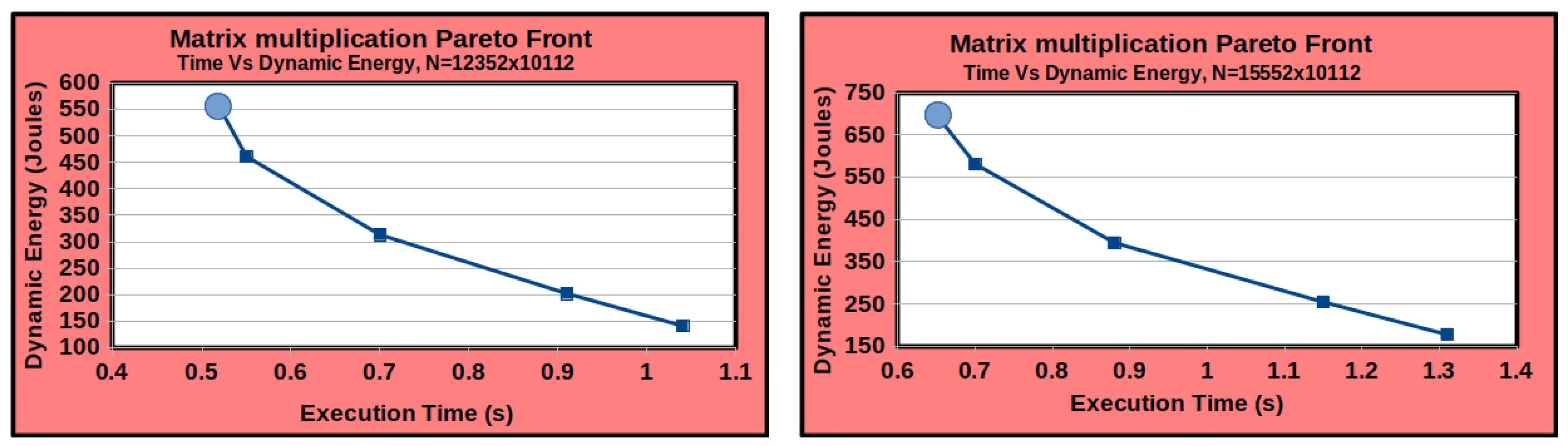
Finally, given the performance or dynamic energy profiles or both, a data-partitioning algorithm solves the single-objective optimization problems for performance or energy or the bi-objective optimization problem for energy and performance to determine the Pareto-optimal solutions (workload distributions), minimizing the execution time and the energy consumption of computations during the parallel execution of the application.
However, two issues hinder the scaling of the proposed optimization methods. We will highlight the issues using as an example the solution method [13] solving the bi-objective optimization problem for energy and performance on p non-linear heterogeneous processors.
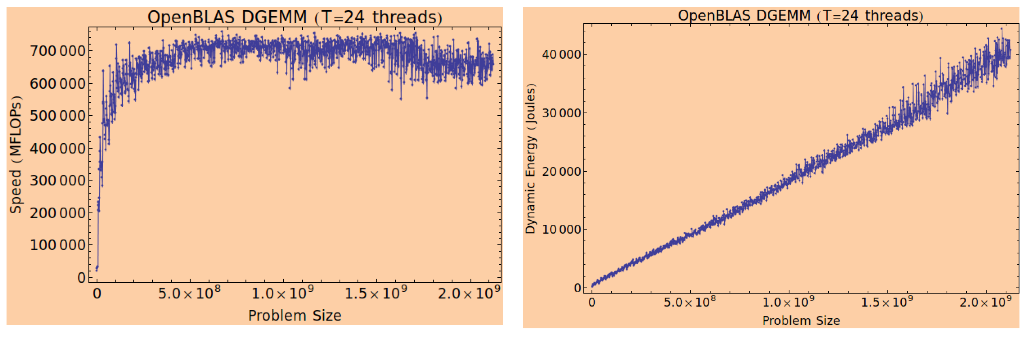
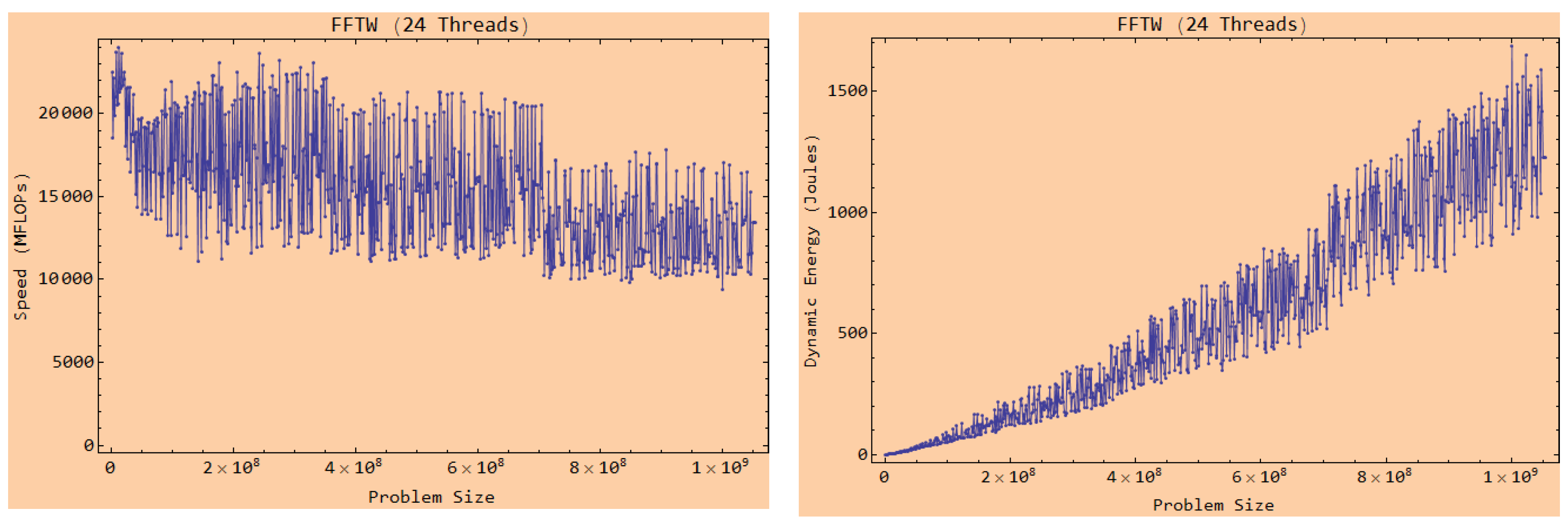
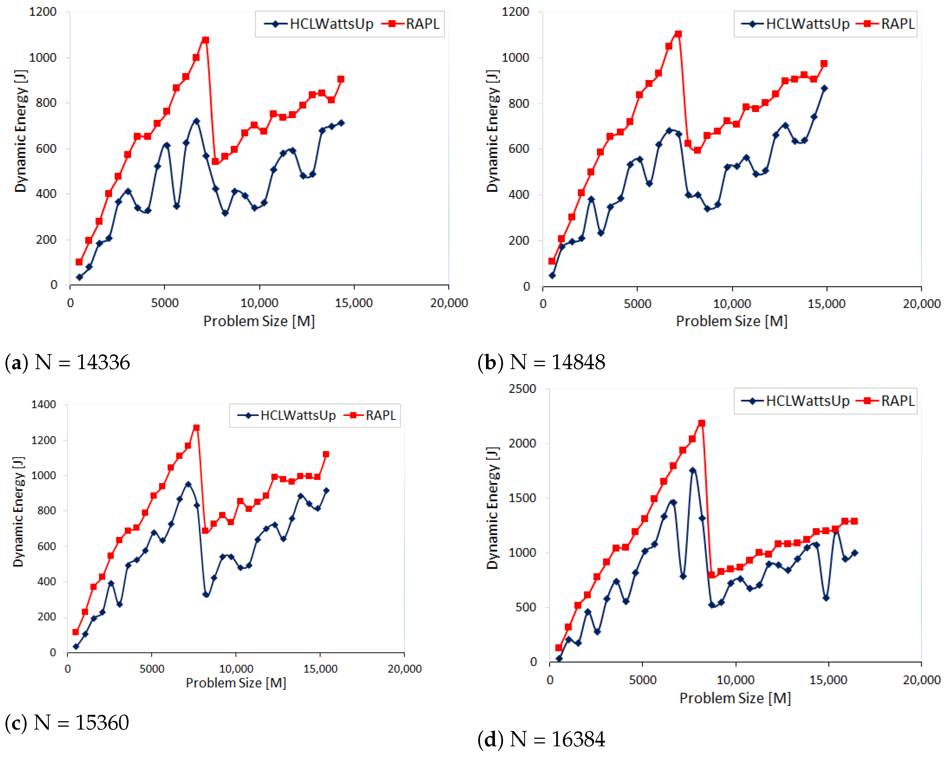
First, constructing the performance and dynamic energy profiles by employing system-level power measurements provided by external power meters (ground-truth method) is sequential and expensive. The execution times of constructing the discrete performance and dynamic energy profiles comprising 210 and 256 workload sizes for the two applications, DGEMM and 2D-FFT, are 8 h and 14 h, respectively. The construction procedure is run on the Intel Skylake processor (
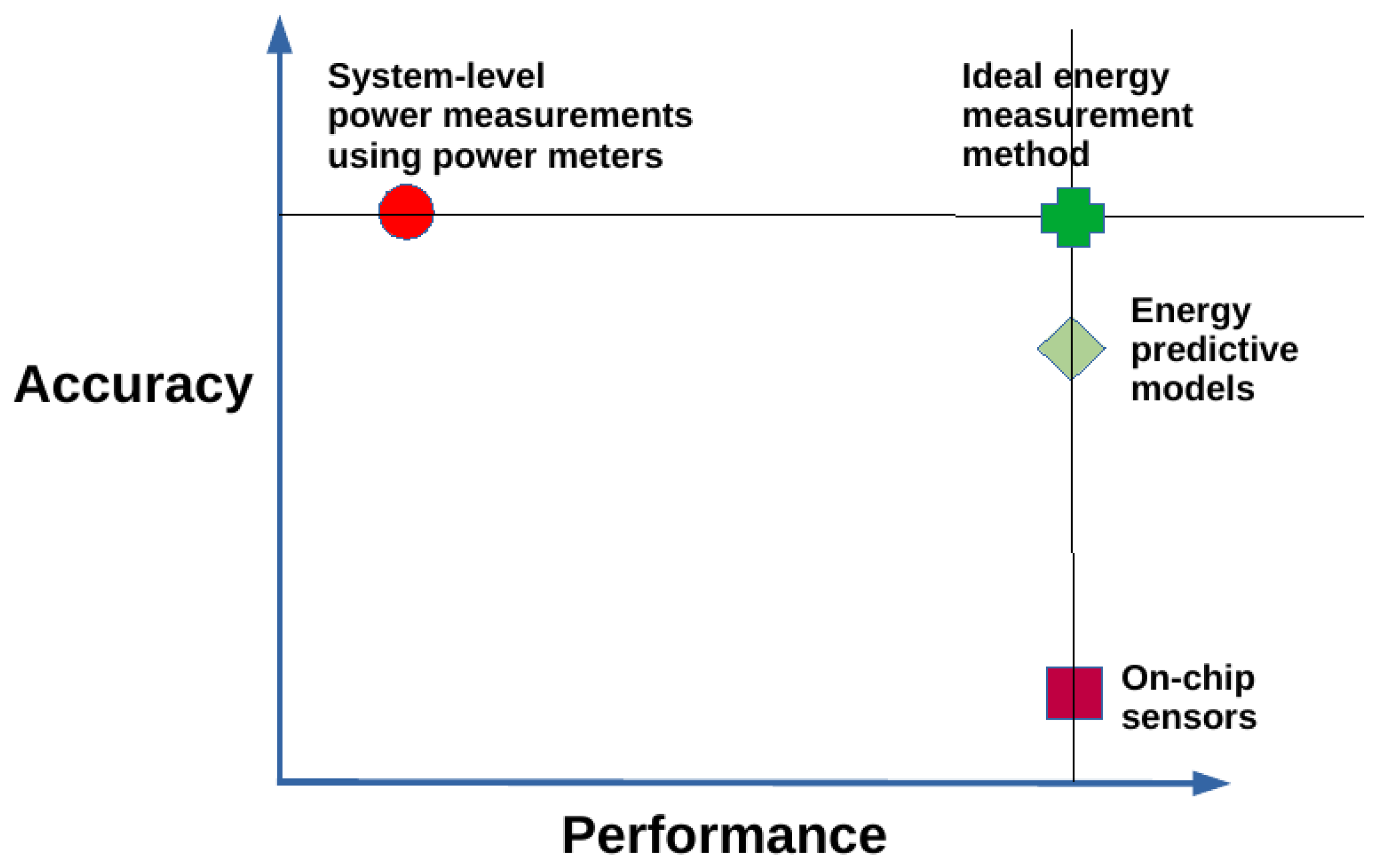
Figure 1). Briefly, while the ground-truth method exhibits the highest accuracy, it is also the most expensive [8]. In addition, it cannot be employed in dynamic environments (HPC platforms and data centers) containing nodes not equipped with power meters.
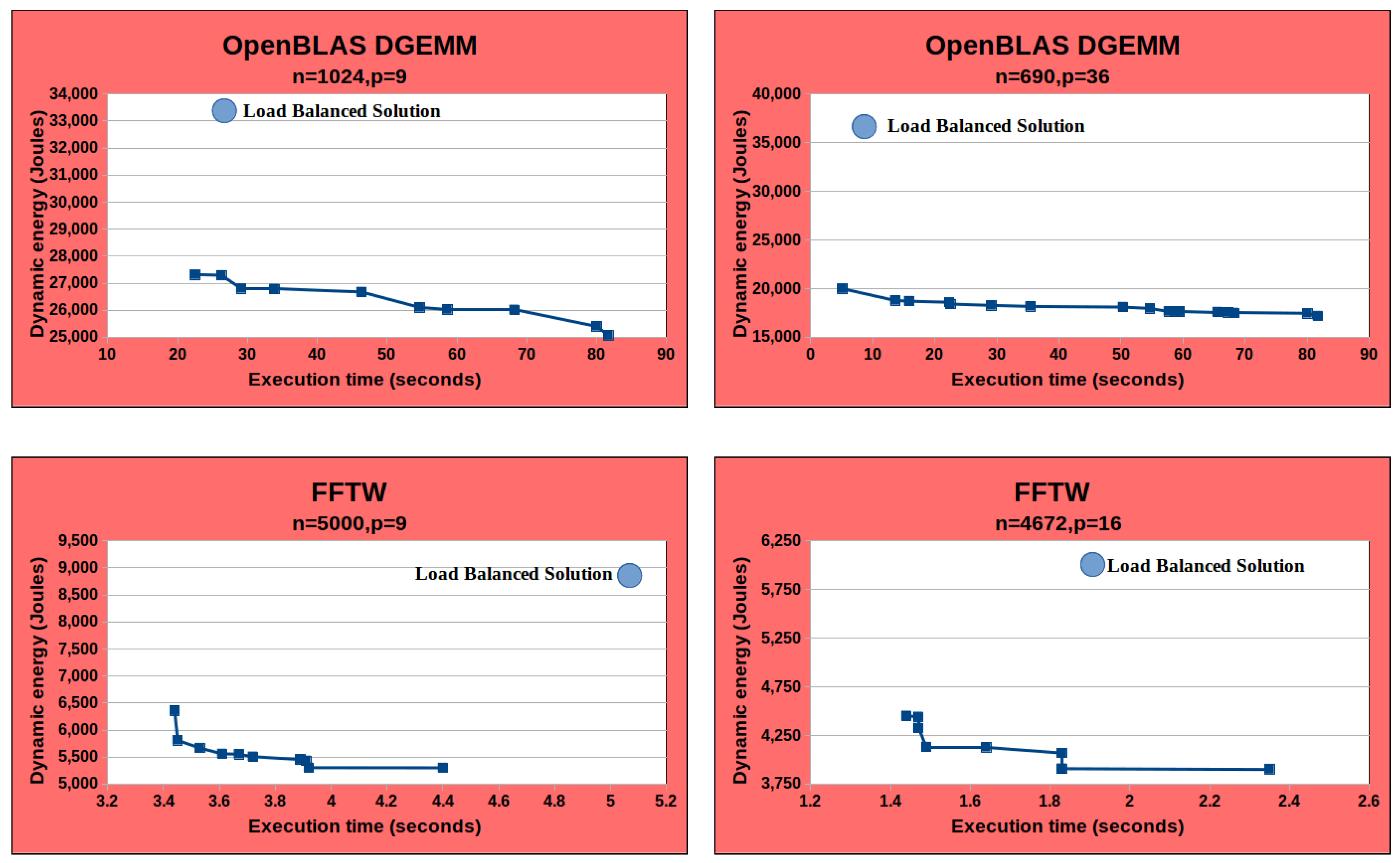
Second, the data-partitioning algorithm is sequential and takes exorbitant execution times for even moderate values of 
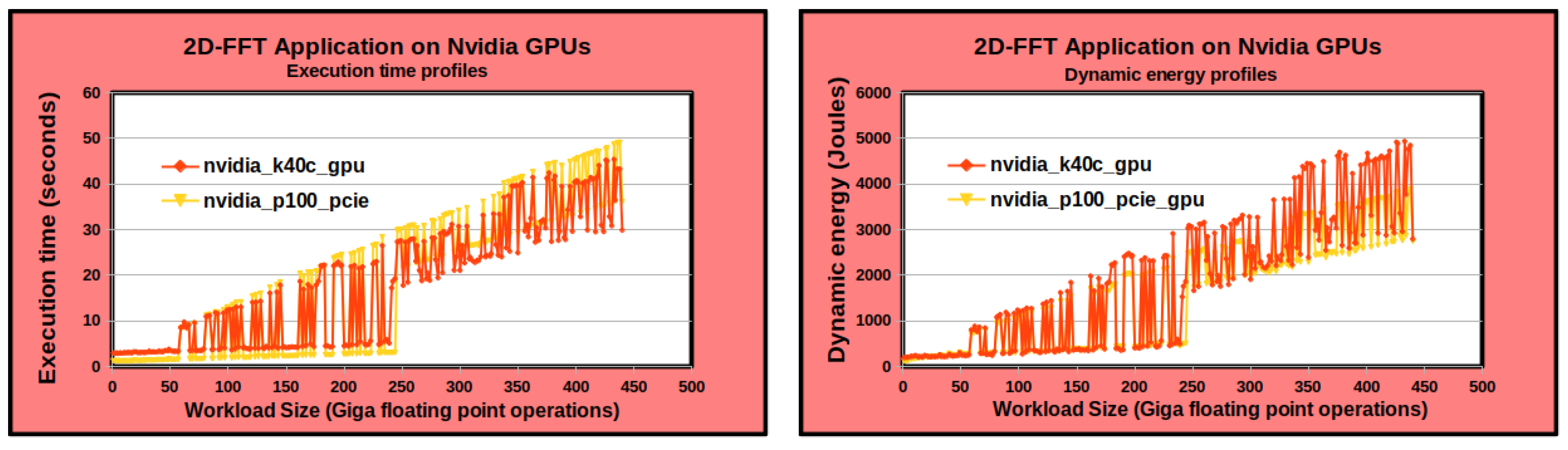
p. For example, consider its execution times for HEPOPTA [13] solving the bi-objective optimization problem for two scientific data-parallel applications, matrix multiplication (DGEMM) and 2D fast Fourier transform (2D-FFT), executed on the hybrid platform (Figure 1). HEPOPTA is sequential and is executed using a single core of the Intel Skylake multicore processor. For the DGEMM application, the data-partitioning algorithm’s execution time ranges from 4 s to 6 h for values of p varying from 12 to 192. For the 2D-FFT application, the execution time increases from 16 s to 16 h for values of p, going from 12 to 192.
Therefore, there are three crucial challenges to accelerating and scaling optimization methods on modern heterogeneous HPC platforms:
  • Acceleration of the sequential optimization algorithms allowing fast runtime computation of Pareto-optimal solutions optimizing the application for performance and energy.
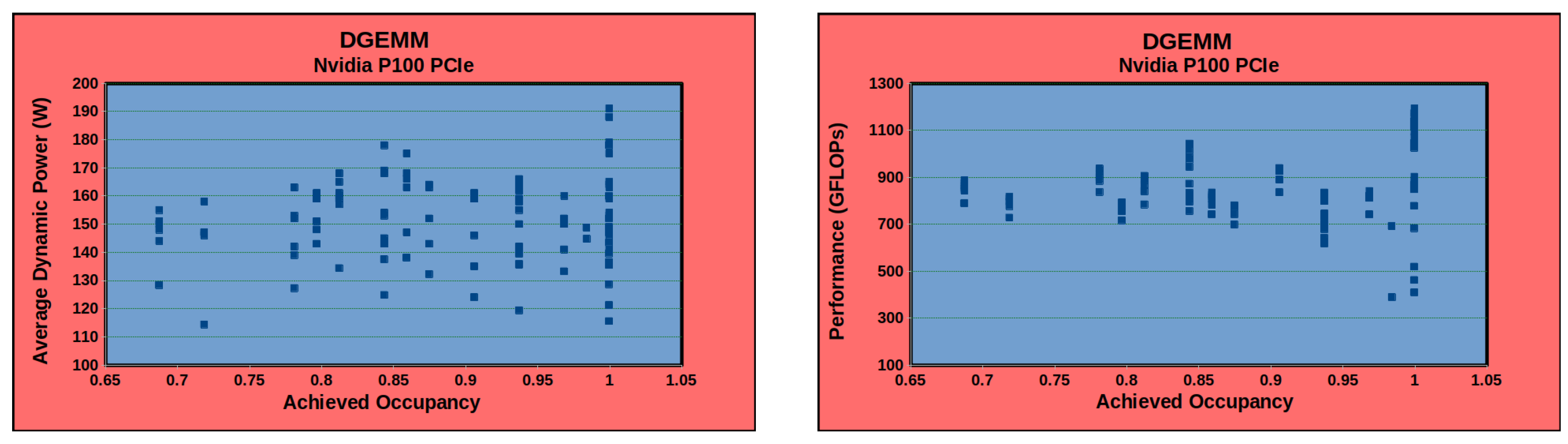
  • Software energy sensors for multicore CPUs and accelerators that are implemented using energy-predictive models employing model variables that are highly additive and satisfying energy conservation laws and based on statistical tests such as high positive correlation.
  • Fast runtime construction of performance and dynamic energy profiles using the software energy sensors.
All three challenges are open problems. However, good progress has been made toward developing software energy sensors for multicore CPUs. For example, the software energy sensor for the Intel multicore CPU can be implemented using a linear energypredictive model based on resource utilization variables and performance monitoring counters (PMCs) that have shown 10-20% accuracy for popular scientific kernels.
Older generations of Nvidia GPUs (Figure 1) were poorly instrumented for runtime energy modeling. However, the latest generation of GPUs, such as Nvidia A40 (Table 1), provide better energy instrumentation support to facilitate the accurate runtime modeling of energy consumption.

7. Concluding Remarks

The paradigm shift in the composition of digital platforms from single-core processors to heterogeneous platforms integrating multicore CPUs and graphics processing units (GPUs) has created significant opportunities for application-level energy optimization and bi-objective optimization for energy and performance. It also engendered two fundamental challenges, non-linearity and heterogeneity.
In this work, we presented an overview of the application-level optimization methods that address the challenges inherent in modern HPC platforms. Applying the methods requires energy profiles of computational kernels (components) of a hybrid parallel application executing on the different computing devices of an HPC platform. Therefore, we summarized the research innovations in the three mainstream component-level energy measurement methods and present their accuracy and performance trade-offs.
Finally, scaling the optimization methods for energy and performance is crucial to achieving energy efficiency objectives and meeting quality-of-service requirements in modern HPC platforms and cloud computing infrastructures. We introduced the building blocks needed to achieve this scaling and concluded with the challenges to scaling. Briefly, two significant challenges are fast optimization methods and accurate component-level energy runtime measurements, especially for components running on accelerators.
Runtime modeling of energy consumption by components running on accelerators is currently in its infancy. So far, the progress in energy modeling concerns CPUs, not accelerators. Older generations of Nvidia GPUs were poorly instrumented for runtime energy modeling. However, the latest generation GPUs, such as Nvidia A40, provide better energy instrumentation support that would facilitate accurate runtime modeling of energy consumption.

Author Contributions

A.L. and R.R.M. have contributed equally. All authors have read and agreed to the published version of the manuscript.

Funding

This publication has emanated from research supported in part by a research grant from Science Foundation Ireland and the Sustainable Energy Authority of Ireland under the SFI Frontiers for the Future Programme 20/FFP-P/8683. This publication has emanated from research conducted with the financial support of the Sustainable Energy Authority of Ireland (SEAI) under Grant Number 21/RDD/664.

Institutional Review Board Statement

Not applicable.

Informed Consent Statement

Not applicable.

Data Availability Statement

Data available on request from the authors.

Acknowledgments

This publication has emanated from research conducted with the financial support of the Sustainable Energy Authority of Ireland (SEAI) under Grant Number 21/RDD/664 and Science Foundation Ireland (SFI) under the SFI Frontiers for the Future Programme 20/FFP-P/8683.

Conflicts of Interest

The authors declare no conflict of interest.

Abbreviations

The following abbreviations are used in this manuscript:
MDPIMultidisciplinary Digital Publishing Institute
ICTInformation and Communications Technology
HPCHigh-performance Computing
DVFSDynamic Voltage and Frequency Scaling
DPMDynamic Power Management
RAPLRunning Average Power Limit
APMAMD Application Power Management
NVMLNVIDIA Management Library
CUPTINVIDIA CUDA Profiling Tools Interface

Appendix A. Optimization for Performance and Energy Using p Identical Linear Parallel Processors

We now prove that any workload distribution between identical linear parallel processors will consume the same dynamic energy, and the load-balanced distribution of the workload will always be optimal for performance and total energy.
Theorem A1.
Consider p identical processors solving a workload n and whose execution time and dynamic energy functions are given by T = { t 1 , t 2 , , t p } , t i ( x ) = a × x and E d = { e d 1 , e d 2 , , e d p } , e d i ( x ) = b × x . Any workload distribution, X = { x 1 , , x p } , i = 1 p x i = n , will consume the same dynamic energy.
Proof. 
Consider an arbitrary workload distribution of n, X = { x 1 , , x p } , i = 1 p x i = n . The total dynamic energy consumption ( E d ) during the execution of the workload n employing X is the following:
E d = e d 1 ( x 1 ) + + e d p ( x p ) = b × x 1 + + b × x p = b × ( x 1 + + x p ) = b × n
Therefore, any workload distribution between identical linear parallel processors will consume the same dynamic energy equal to b × n . □
Theorem A2.
Consider p identical processors solving a workload n and whose execution time and dynamic energy functions are given by T = { t 1 , t 2 , , t p } , t i ( x ) = a × x and E d = { e d 1 , e d 2 , , e d p } , e d i ( x ) = b × x . Let us assume the static power consumption of a processor is P s . Then, the load-balanced distribution of the workload is optimal for performance and total energy.
Proof. 
Consider the load-balanced distribution of the workload n, X l b = { x 1 , , x p } , i = 1 p x i = n . By the definition of load-balanced distribution, t 1 ( x 1 ) = = t p ( x p ) a × x 1 = = a × x p x 1 = = x p . Therefore, the load-balanced distribution is also the load-equal distribution, and the total execution time during the execution of the workload n is equal to any of the execution times, { a × x 1 , , a × x p } .
Consider an arbitrary workload distribution, Y = { y 1 , , y p } , i = 1 p y i = n , other than X l b . Let us assume that processor k takes the longest time t k in solving the workload size, y k , assigned to it. By definition, t k ( y k ) > t i ( x i ) a × y k > a × x i y k > x i . Therefore, the total execution time during the execution of the workload n employing Y is equal to the following:
T = min max ( t 1 ( y 1 ) , , t p ( y p ) ) = min t k ( y k ) = t k ( y k ) > t i ( x i ) i { 1 , , p }
Hence, the load-balanced distribution X l b is optimal for performance.
Since by Theorem 1, any workload distribution between identical linear parallel processors will consume the same dynamic energy equal to b × n , X l b will also consume the same amount of dynamic energy. The total energy consumption ( E T ) during the execution of the workload n employing X l b is the following:
E T = P s × t 1 ( x 1 ) + + P s × t p ( x p ) + b × n = P s × ( a × x 1 + + a × x p ) + b × n = P s × a × ( x 1 + + x p ) + b × n = P s × a × n + b × n
Following on similar lines, consider again an arbitrary workload distribution, Y = { y 1 , , y p } , i = 1 p y i = n , other than X l b . Let us assume that processor k takes the longest time t k in solving the workload size, y k , assigned to it. The total energy consumption ( E T ) during the execution of the workload n employing Y is the following:
E T = P s × t k ( y k ) + + P s × t k ( y k ) + b × n = P s × a × ( y k + + y k ) + b × n = P s × a × n × y k + b × n > P s × a × n + b × n
Therefore, the load-balanced distribution X l b is optimal for total energy. □

Appendix B. Optimization for Performance and Energy Using p Heterogeneous Linear Parallel Processors

We illustrate the study’s findings [14] using a highly optimized matrix multiplication application executing on a heterogeneous computing platform shown in Figure 1. The application computes the matrix product, C = α × A × B + β × C , where A, B, and C are matrices of size M × N , N × N , and M × N , respectively, and α and β are constant floating-point numbers. The application invokes CUBLAS library functions for Nvidia GPUs and Intel MKL DGEMM library functions for CPUs and Intel Xeon Phi. The Intel MKL and CUDA versions used are 2017.0.2 and 9.2.148.
The platform consists of five heterogeneous processors: Intel Haswell E5-2670V3 multi-core CPU, Intel Xeon Gold 6152 multi-core CPU, NVIDIA K40c GPU, NVIDIA P100 PCIe GPU, and Intel Xeon Phi 3120P. In addition, the platform has five heterogeneous abstract processors, CPU_1, GPU_1, xeonphi_1, CPU_2, and GPU_2, each executing a computational kernel.
Figure A1 shows the execution time and dynamic energy functions of the processors against the workload size that ranges from 64 × 10,112 to 19,904 × 10,112 with a step size of 64 for the first dimension M. The static and dynamic energy consumption during the application execution is obtained using the ground-truth method. The shapes of the execution time functions are continuous and strictly increasing. The shapes of the energy functions can be approximated accurately by linear increasing functions.
Figure A1. The figures in the left column show the execution time and energy profiles of the five heterogeneous processors (Figure 1) employed in the matrix multiplication application. The figures in the right column exclude the Xeon Phi profiles since its energy profile dominates the other energy profiles. Note that the execution time profiles of CPU_1 and CPU_2 are close to each other. However, the energy profile of CPU_1 is significantly higher than that of CPU_2.
Information 14 00248 g0a1
Figure A2 shows the Pareto fronts obtained using the algorithms proposed in [14] for the matrix multiplication application for two workloads, 12,352 × 10,112 and 15,552 × 10,112. The algorithms take input performance and dynamic energy functions that are linear approximations of the profiles. Each Pareto front contains four linear segments. The solution (shown as a circle) with minimal execution time is the load-balancing solution.
Figure A2. Pareto fronts for the matrix multiplication application executing on the heterogeneous platform (Figure 1) for two workloads. Each Pareto front contains four linear segments.
Information 14 00248 g0a2

Appendix C. Intel RAPL

Running Average Power Limit (RAPL) [22] provided in Intel multicore CPUs allows for monitoring power and controlling frequency (and voltage). In addition, for processor generations preceding Haswell, such as Sandybridge and Ivybridge E5, it employs a software model using performance monitoring counters (PMCs) as predictor variables to measure energy consumption for CPUs and DRAM [44].
However, for Haswell and later processor generations, RAPL uses separate voltage regulators (VR IMON) for CPU and DRAM. VR IMON is an analog circuit within a voltage regulator (VR). It keeps track of the current estimate. However, there is a latency between the measured current-sense signal and the actual current signal to the CPU, which may affect the accuracy of the readings. The CPU samples this reading periodically (100 μ s to 1 ms) for calculating the power [45].
RAPL provides energy counters in model-specific registers (MSRs). It divides a platform into power domains for fine-grained control. These domains include Package, which includes core and uncore components; DRAM, which is is available only for servers; and CPU cores, the graphics component of the CPU (uncore).
References [26,45] cite systematic errors in RAPL energy counters that are rectified to some extent due to the use of VR IMON for power measurement [46].
We present the findings by Fahad et al. [8]. The authors study the optimization of a parallel matrix multiplication application for dynamic energy using Intel RAPL and the ground-truth method. The ground-truth method comprises system-level physical power measurements obtained using the HCLWattsUp API. The study demonstrates that using Intel RAPL leads to significant energy losses.
The parallel application multiplies two dense square matrices A and B of size N × N and is executed on the two Intel multicore CPU processors shown in Figure 1, Intel Haswell E5-2670V3 (CPU1) and Intel Xeon Gold 6152 (CPU2). Matrix B is replicated at both processors. CPU1 computes the product of matrices A 1 and B, while CPU2 computes the product of matrices A 2 and B. The local matrix products are computed using the Intel MKL DGEMM routine. There are no communications involved.
The matrix A is partitioned into A 1 and A 2 of sizes M × N and K × N between the processors using a model-based data partitioning algorithm where M + K = N .
The algorithm takes as input the matrix size, N, and the discrete dynamic energy functions of the processors, e 1 ( x , y ) and e 2 ( x , y ) . e i ( x , y ) gives the dynamic energy consumption of matrix multiplication of matrices of sizes x × y and y × y . Therefore, the dynamic energy function is represented by a surface. The algorithm outputs M and K.
Informally, the algorithm cuts the surfaces of the dynamic energy functions by a plane y = N . The cut produces two curves. It then determines two points on the curves, ( M , e 1 ( M , N ) ) and ( K , e 2 ( K , N ) ) , whose sum of energy consumptions, e 1 ( M , N ) + e 2 ( K , N ) , is minimal.
Figure A3 illustrates the dynamic energy profiles for four workload sizes (N), {14,336, 14,848, 15,360, 16,384}, using RAPL and HCLWattsUp, respectively.
Figure A3. Dynamic energy consumption profiles of DGEMM on the two Intel multicore CPU processors.
Information 14 00248 g0a3
Intel RAPL reports more dynamic energy consumption than the ground truth for all the workload sizes. The prediction errors of Intel RAPL are tabulated in Table A1. The average errors are { 65 % , 58 % , 56 % , 56 % } .
Table A1. Prediction errors of Intel RAPL against ground-truth for dynamic energy consumption by DGEMM.
Workload Size (N)MinMaxAvg
14,33617%172%65%
14,84812%153%58%
15,36013%240%56%
16,3842%300%56%
The data-partitioning algorithm determines the workload distribution using the inputs, workload size N and the dynamic energy profiles of the two processors. Then, the dynamic energy consumption is obtained by executing the parallel application using the workload distribution. The dynamic energy losses (in percent) incurred by employing Intel RAPL for the four workload sizes are { 54 , 37 , 31 , 84 } .

Appendix D. Accuracy of MPSS against Ground Truth on Intel Xeon Phi Co-Processor

Table A2 compares the accuracy of MPSS for Intel MKL DGEMM and Intel MKL FFT applications against the ground-truth method. Using calibration, the average and maximum errors can be reduced to 9.58% and 32.3%, respectively. Calibration is a constant adjustment made to all the points in a dynamic energy profile to improve its accuracy against the ground truth.
Table A2. Percentage error of MPSS against ground-truth dynamic energy profiles with and without calibration on the Intel Xeon Phi co-processor (Figure 1) for Intel MKL DGEMM and Intel MKL FFT applications.
Without Calibration
ApplicationMinMaxAvg
Intel MKL DGEMM45.1%93.06%64.5%
Intel MKL FFT22.58%55.78%40.68%
With Calibration
ApplicationMinMaxAvg
Intel MKL DGEMM0.06%9.54%2.75%
Intel MKL FFT0.06%32.3%9.58%

Appendix E. Accuracy of NVML against Ground-Truth on Nvidia K40c GPU and Nvidia P100 PCIe

Table A3 and Table A4 illustrate the errors using NVML with and without using calibration on Nvidia K40c and Nvidia P100 PCIe GPUs (Figure 1).
Table A3. Percentage error of dynamic energy consumption obtained using NVML against ground-truth on Nvidia K40c GPU (Figure 1) with and without calibration.
Without Calibration
ApplicationMinMaxAvg
CUBLAS DGEMM0.076%35.32%10.62%
CUBLAS FFT0.52%57.77%12.45%
With Calibration
ApplicationMinMaxAvg
CUBLAS DGEMM0.19%30.50%10.43%
CUBLAS FFT0.18%94.55%10.87%
Table A4. Percentage error of dynamic energy consumption obtained using NVML against the ground truth on Nvidia P100 PCIe GPU (Figure 1) with and without calibration.
Without Calibration
ApplicationMinMaxAvg
CUBLAS DGEMM13.11%84.84%40.06%
CUBLAS FFT17.91%175.97%73.34%
With Calibration
ApplicationMinMaxAvg
CUBLAS DGEMM0.07%26.07%11.62%
CUBLAS FFT0.025%51.24%16.95%

Appendix F. Additivity of Performance Monitoring Counters (PMCs)

The additivity error of a PMC is determined using a procedure. The input to the procedure is a dataset of applications, which are called base applications. The dataset of applications is a collection of well-known benchmarks, highly optimized scientific kernels, and naive unoptimized scientific routines. An example of such a collection is given in [32].
Using the input dataset, a dataset of compound applications is composed. Each compound application is a serial execution of two base applications.
For each compound application in the dataset, the PMC counts for the base applications and the compound application are obtained. The PMC error for the compound application is calculated as follows:
E r r o r ( % ) = | ( e b 1 + e b 2 ) e c ( e b 1 + e b 2 + e c ) / 2 | × 100
where e c , e b 1 , e b 2 are the PMC counts for the compound and constituent base applications, respectively. The sample average of this error is obtained from multiple experimental runs of the compound and base applications.
The additivity error of the PMC is the maximum of errors for all the compound applications in the dataset.

Appendix G. Selection of Model Variables Based on Energy Conservation Laws

We present a review of the theory of energy predictive models of computing proposed in [32]. The theory formalizes properties of PMC-based energy predictive models that are derived from the fundamental physical law of energy conservation. The properties capture the essence of single application runs and characterize the behavior of serial execution of two applications. A PMC vector represents an application run. A null PMC vector contains zeroes for all its PMC values.
The properties are intuitive and experimentally validated. The formulations of the properties are based on the following observations:
  • In a dedicated and stable environment, the PMC vector of the serial execution of two applications will always be the same if the same PMC vector represents each application run.
  • An application run that does not consume energy has a null PMC vector.
  • An application with a non-null PMC vector must consume some energy.
  • Finally, the consumed energy of a compound application is equal to the sum of the energies consumed by the individual applications.
The theory provides practical implications for constructing accurate and reliable linear energy-predictive models. They include selection criteria for model variables, model intercept, and model coefficients that are outlined below:
  • Each model variable must be deterministic and reproducible.
  • Each model variable must be additive.
  • The model intercept must be zero.
  • Each model coefficient must be positive.
The first two properties form the additivity test for selecting PMCs. Therefore, a PMC-based linear energy-predictive model that violates the criteria will have poor prediction accuracy.

Appendix H. Best Linear Energy Predictive Models for Intel Multicore CPUs

Shahid et al. [34] propose linear models employing processor and memory utilizations and PMCs as model variables.
The processor utilization model variable, u p r o c e s s o r , is given by the equation below:
u p r o c e s s o r = ( U ˜ p r o c e s s o r / 100 ) × T D P p r o c e s s o r × t
The parameter U ˜ p r o c e s s o r is the processor utilization. It is the proportion of time the processor is busy doing work divided by the total amount of time. The parameter T D P p r o c e s s o r is the theoretical maximum power consumed by the processor, also known as the thermal design power, TDP. The product of the two parameters gives an estimate of the average power consumption by the processor. The model variable u p r o c e s s o r that multiplies this product by the application’s execution time (t) represents the energy consumption. The details of obtaining the processor utilization are given in [47].
Similarly, the memory utilization model variable, u m e m o r y , is determined using the equation below:
u m e m o r y = ( U ˜ m e m o r y / 100 ) × T D P m e m o r y × t
The parameters U ˜ m e m o r y and T D P m e m o r y are the memory utilization and the thermal design power of the memory (DRAM).
The mathematical form of the dynamic energy predictive models employing both utilization variables and PMCs is shown below:
E u p m c = α 1 × u p r o c e s s o r + α 2 × u m e m o r y + β 1 × p m c 1 + + β n × p m c n
where E u p m c is the dynamic energy consumption and { α 1 , α 2 , β 1 , . . . , β n } are the regression coefficients or the model parameters.

References

  1. Andrae, A. New perspectives on internet electricity use in 2030. Eng. Appl. Sci. Lett. 2020, 3, 19–31. [Google Scholar]
  2. Lastovetsky, A.; Reddy, R. New Model-Based Methods and Algorithms for Performance and Energy Optimization of Data Parallel Applications on Homogeneous Multicore Clusters. IEEE Trans. Parallel Distrib. Syst. 2017, 28, 1119–1133. [Google Scholar] [CrossRef]
  3. Reddy, R.; Lastovetsky, A. Bi-Objective Optimization of Data-Parallel Applications on Homogeneous Multicore Clusters for Performance and Energy. IEEE Trans. Comput. 2018, 67, 160–177. [Google Scholar]
  4. Miettinen, K. Nonlinear Multiobjective Optimization; Springer: New York, NY, USA, 1998. [Google Scholar]
  5. Talbi, E.G. Metaheuristics: From Design to Implementation; John Wiley & Sons: Hoboken, NJ, USA, 2009; Volume 74. [Google Scholar]
  6. Fahad, M.; Manumachu, R.R. HCLWattsUp: Energy API Using System-Level Physical Power Measurements Provided by Power Meters; Heterogeneous Computing Laboratory, University College Dublin: Dublin, Ireland, 2023. [Google Scholar]
  7. OpenBLAS. OpenBLAS: An Optimized BLAS Library. Available online: https://github.com/xianyi/OpenBLAS (accessed on 1 December 2022).
  8. Fahad, M.; Shahid, A.; Reddy, R.; Lastovetsky, A. A Comparative Study of Methods for Measurement of Energy of Computing. Energies 2019, 12, 2204. [Google Scholar] [CrossRef]
  9. Top500. The Top500 Supercomputers List. Available online: https://www.top500.org (accessed on 1 December 2022).
  10. Krommydas, K.; Feng, W.C.; Antonopoulos, C.D.; Bellas, N. OpenDwarfs: Characterization of Dwarf-Based Benchmarks on Fixed and Reconfigurable Architectures. J. Signal Process. Syst. 2016, 85, 373–392. [Google Scholar] [CrossRef]
  11. Kreutzer, M.; Thies, J.; Röhrig-Zöllner, M.; Pieper, A.; Shahzad, F.; Galgon, M.; Basermann, A.; Fehske, H.; Hager, G.; Wellein, G. GHOST: Building Blocks for High Performance Sparse Linear Algebra on Heterogeneous Systems. Int. J. Parallel Program. 2016, 45, 1046–1072. [Google Scholar] [CrossRef]
  12. Papadrakakis, M.; Stavroulakis, G.; Karatarakis, A. A new era in scientific computing: Domain decomposition methods in hybrid CPU–GPU architectures. Comput. Methods Appl. Mech. Eng. 2011, 200, 1490–1508. [Google Scholar] [CrossRef]
  13. Khaleghzadeh, H.; Fahad, M.; Shahid, A.; Reddy, R.; Lastovetsky, A. Bi-Objective Optimization of Data-Parallel Applications on Heterogeneous HPC Platforms for Performance and Energy Through Workload Distribution. IEEE Trans. Parallel Distrib. Syst. 2021, 32, 543–560. [Google Scholar] [CrossRef]
  14. Khaleghzadeh, H.; Reddy, R.; Lastovetsky, A. Efficient exact algorithms for continuous bi-objective performance-energy optimization of applications with linear energy and monotonically increasing performance profiles on heterogeneous high performance computing platforms. Concurr. Comput. Pract. Exp. 2022, e7285. [Google Scholar] [CrossRef]
  15. FFTW. FFTW: A Fast, Free C FFT Library. Available online: https://www.fftw.org (accessed on 1 December 2022).
  16. Lastovetsky, A.L.; Reddy, R. Data partitioning with a realistic performance model of networks of heterogeneous computers. In Proceedings of the Parallel and Distributed Processing Symposium, Hong Kong, China, 13–15 December 2004. [Google Scholar]
  17. Lastovetsky, A.; Reddy, R. Data partitioning with a functional performance model of heterogeneous processors. Int. J. High Perform. Comput. Appl. 2007, 21, 76–90. [Google Scholar] [CrossRef]
  18. Lastovetsky, A.; Twamley, J. Towards a realistic performance model for networks of heterogeneous computers. In High Performance Computational Science and Engineering; Springer: Berlin, Germany, 2005; pp. 39–57. [Google Scholar]
  19. Khaleghzadeh, H.; Reddy, R.; Lastovetsky, A. A novel data-partitioning algorithm for performance optimization of data-parallel applications on heterogeneous HPC platforms. IEEE Trans. Parallel Distrib. Syst. 2018, 29, 2176–2190. [Google Scholar] [CrossRef]
  20. Khaleghzadeh, H.; Fahad, M.; Reddy, R.; Lastovetsky, A. A novel data partitioning algorithm for dynamic energy optimization on heterogeneous high-performance computing platforms. Concurr. Comput. Pract. Exp. 2020, 32, e5928. [Google Scholar] [CrossRef]
  21. Fahad, M.; Shahid, A.; Manumachu, R.R.; Lastovetsky, A. Accurate Energy Modelling of Hybrid Parallel Applications on Modern Heterogeneous Computing Platforms Using System-Level Measurements. IEEE Access 2020, 8, 93793–93829. [Google Scholar] [CrossRef]
  22. Rotem, E.; Naveh, A.; Ananthakrishnan, A.; Weissmann, E.; Rajwan, D. Power-Management Architecture of the Intel Microarchitecture Code-Named Sandy Bridge. IEEE Micro 2012, 32, 20–27. [Google Scholar] [CrossRef]
  23. Treibig, J.; Hager, G.; Wellein, G. Likwid: A lightweight performance-oriented tool suite for x86 multicore environments. In Proceedings of the Parallel Processing Workshops (ICPPW), San Diego, CA, USA, 13–16 September 2010; pp. 207–216. [Google Scholar]
  24. Devices, A.M. AMD uProf User Guide. Available online: https://www.amd.com/content/dam/amd/en/documents/developer/uprof-v4.0-gaGA-user-guide.pdf (accessed on 1 December 2022).
  25. Devices, A.M. BIOS and Kernel Developer’s Guide (BKDG) for AMD Family 15h Models 00h-0Fh Processors. Available online: https://www.amd.com/system/files/TechDocs/42301_15h_Mod_00h-0Fh_BKDG.pdf (accessed on 1 December 2022).
  26. Hackenberg, D.; Ilsche, T.; Schöne, R.; Molka, D.; Schmidt, M.; Nagel, W.E. Power measurement techniques on standard compute nodes: A quantitative comparison. In Proceedings of the 2013 IEEE International Symposium on Performance Analysis of Systems and Software (ISPASS), Austin, TX, USA, 21–23 April 2013; pp. 194–204. [Google Scholar]
  27. Intel Corporation. Intel Xeon Phi Coprocessor System Software Developers Guide. Available online: https://www.intel.com/content/dam/develop/external/us/en/documents/intel-xeon-phi-coprocessor-quick-start-developers-guide-windows-v1-2.pdf (accessed on 1 December 2022).
  28. Intel Corporation. Intel Manycore Platform Software Stack (Intel MPSS). Available online: https://www.intel.com/content/www/us/en/developer/articles/tool/manycore-platform-software-stack-mpss.html (accessed on 1 December 2022).
  29. Nvidia. Nvidia Management Library: NVML API Reference Guide. Available online: https://docs.nvidia.com/deploy/nvml-api/index.html (accessed on 1 December 2022).
  30. O’Brien, K.; Pietri, I.; Reddy, R.; Lastovetsky, A.; Sakellariou, R. A Survey of Power and Energy Predictive Models in HPC Systems and Applications. ACM Comput. Surv. 2017, 50, 1–38. [Google Scholar] [CrossRef]
  31. Shahid, A.; Fahad, M.; Reddy, R.; Lastovetsky, A. Additivity: A Selection Criterion for Performance Events for Reliable Energy Predictive Modeling. Supercomput. Front. Innov. Int. J. 2017, 4, 50–65. [Google Scholar]
  32. Shahid, A.; Fahad, M.; Reddy, R.; Lastovetsky, A.L. Energy Predictive Models of Computing: Theory, Practical Implications and Experimental Analysis on Multicore Processors. IEEE Access 2021, 9, 63149–63172. [Google Scholar] [CrossRef]
  33. Shahid, A.; Fahad, M.; Reddy, R.; Lastovetsky, A. Improving the Accuracy of Energy Predictive Models for Multicore CPUs Using Additivity of Performance Monitoring Counters. In Proceedings of the Parallel Computing Technologies; Malyshkin, V., Ed.; Springer International Publishing: Cham, Switzerland, 2019; pp. 51–66. [Google Scholar]
  34. Shahid, A.; Fahad, M.; Manumachu, R.R.; Lastovetsky, A. Improving the accuracy of energy predictive models for multicore CPUs by combining utilization and performance events model variables. J. Parallel Distrib. Comput. 2021, 151, 38–51. [Google Scholar] [CrossRef]
  35. NVIDIA Corporation. CUDA Profiling Tools Interface (CUPTI)—1.0. Available online: https://developer.nvidia.com/cuda-profiling-tools-interface (accessed on 1 December 2022).
  36. Nagasaka, H.; Maruyama, N.; Nukada, A.; Endo, T.; Matsuoka, S. Statistical power modeling of GPU kernels using performance counters. In Proceedings of the International Green Computing Conference and Workshops (IGCC), Chicago, IL, USA, 15–18 August 2010. [Google Scholar]
  37. Zhang, Y.; Hu, Y.; Li, B.; Peng, L. Performance and Power Analysis of ATI GPU: A Statistical Approach. In Proceedings of the IEEE Sixth International Conference on Networking, Architecture, and Storage, IEEE Computer Society, Washington, DC, USA, 28–30 July 2011; pp. 149–158. [Google Scholar]
  38. Song, S.; Su, C.; Rountree, B.; Cameron, K.W. A Simplified and Accurate Model of Power-Performance Efficiency on Emergent GPU Architectures. In Proceedings of the 27th IEEE International Parallel and Distributed Processing Symposium (IPDPS), Cambridge, MA, USA, 20–24 May 2013; pp. 673–686. [Google Scholar]
  39. Al-Hashimi, M.; Saleh, M.; Abulnaja, O.; Aljabri, N. Evaluation of control loop statements power efficiency: An experimental study. In Proceedings of the 2014 9th International Conference on Informatics and Systems, Cairo, Egypt, 15–17 December 2014; pp. PDC-45–PDC-48. [Google Scholar]
  40. Coplin, J.; Burtscher, M. Effects of Source-Code Optimizations on GPU Performance and Energy Consumption. In Proceedings of the 8th Workshop on General Purpose Processing Using GPUs, San Francisco, CA, USA, 7 February 2015; pp. 48–58. [Google Scholar]
  41. Lee, S.; Kim, K.; Koo, G.; Jeon, H.; Ro, W.W.; Annavaram, M. Warped-Compression: Enabling power efficient GPUs through register compression. In Proceedings of the 2015 ACM/IEEE 42nd Annual International Symposium on Computer Architecture (ISCA), Portland, OR, USA, 13–17 June 2015; pp. 502–514. [Google Scholar]
  42. Ikram, M.J.; Saleh, M.E.; Al-Hashimi, M.A.; Abulnaja, O.A. Investigating the effect of varying block size on power and energy consumption of GPU kernels. J. Supercomput. 2022, 78, 14919–14939. [Google Scholar] [CrossRef]
  43. Zhong, Z.; Rychkov, V.; Lastovetsky, A. Data partitioning on multicore and multi-GPU platforms using functional performance models. Comput. IEEE Trans. 2015, 64, 2506–2518. [Google Scholar] [CrossRef]
  44. David, H.; Gorbatov, E.; Hanebutte, U.R.; Khanna, R.; Le, C. RAPL: Memory power estimation and capping. In Proceedings of the 2010 ACM/IEEE International Symposium on Low-Power Electronics and Design (ISLPED), Austin, TX, USA, 18–20 August 2010; pp. 189–194. [Google Scholar]
  45. Gough, C.; Steiner, I.; Saunders, W. Energy Efficient Servers Blueprints for Data Center Optimization; Apress: New York, NY, USA, 2015. [Google Scholar]
  46. Hackenberg, D.; Schöne, R.; Ilsche, T.; Molka, D.; Schuchart, J.; Geyer, R. An Energy Efficiency Feature Survey of the Intel Haswell Processor. In Proceedings of the 2015 IEEE International Parallel and Distributed Processing Symposium Workshop, Washington, DC, USA, 25–29 May 2015; pp. 896–904. [Google Scholar]
  47. Reddy, R.; Lastovetsky, A. On Energy Nonproportionality of CPUs and GPUs. In Proceedings of the 2022 IEEE International Parallel and Distributed Processing Symposium Workshops (IPDPSW), Lyon, France, 30 May–3 June 2022; pp. 34–44. [Google Scholar] [CrossRef]
Figure 1. Specifications of the five heterogeneous processors, Intel Haswell multicore CPU, Nvidia K40c, Intel Xeon Phi 3120P, Intel Skylake multicore CPU and Nvidia P100 PCIe.
Information 14 00248 g001
Figure 2. Execution time and dynamic energy profiles of OpenBLAS DGEMM application multiplying two square matrices of size n × n on a single core of the Intel Haswell multicore CPU shown in Figure 1. The application is multithreaded and uses only one thread during its execution. The workload size shown on the x-axis equals 2 × n 3 . The workload is shown in Giga floating point operations. The y-axis in the left-hand and right-hand plots show the execution time and dynamic energy consumption of the computations involved in matrix multiplication in the OpenBLAS DGEMM application. The execution time and dynamic energy profiles observed are linear functions of workload size.
Information 14 00248 g002
Figure 3. Solving bi-objective optimization problems for two processors with linear execution time and energy functions results in a linear Pareto front. The endpoints of the front are the solutions for single-objective optimization for performance and energy. (a). Linear execution time functions of workload size of the processors P 1 and P 2 . The units for workload size on the x-axis are Giga floating point operations. (b). Linear energy functions of workload size of the processors P 1 and P 2 . The units for workload size on the x-axis are Giga floating point operations. (c). Pareto-optimal solutions for a workload size 348.
Information 14 00248 g003
Figure 4. Consider the bi-objective optimization problem for performance and energy for p heterogeneous processors characterized by p linear increasing time functions, { f 0 , , f p 1 } , in set F, and p linear increasing energy functions, { g 0 , , g p 1 } in set G. (a). The set of p linear increasing time functions, { f 0 , , f p 1 } , in set F. (b). The set of p linear increasing energy functions, { g 0 , , g p 1 } in set G. (c). The algorithm proposed in [14] solves the problem and returns a piecewise linear Pareto front comprising a chain of p 1 linear segments, { S 0 , , S p 2 } .
Information 14 00248 g004
Figure 5. The speed and dynamic energy consumption profiles for the OpenBLAS DGEMM application employing 24 threads on the Intel Haswell multicore CPU are shown in Figure 1. The application multiplies two matrices of size x × n and n × n where n is 46,080. The problem size in the figure is x × n . The workload size 2 × x × n 2 is proportional to the problem size (since n is kept constant). Note the non-linear profile shapes in the plots are observed for many matrix sizes. We have selected one matrix size (n = 46,080) only for illustration.
Information 14 00248 g005
Figure 6. The speed and dynamic energy consumption profiles for the FFTW application employing 24 threads on the Intel Haswell multicore CPU are shown in Figure 1. The application computes a 2D fast Fourier transform (FFT) of a dense signal matrix of size n × n . The problem size on the x-axis is n 2 . The workload size is 5 × n 2 × log 2 n . Therefore, the speed and dynamic energy profiles versus workload size will still be highly non-linear.
Information 14 00248 g006
Figure 7. The speed (MFLOPs) and dynamic energy consumption profiles of OpenBLAS DGEMM application executing a varying number of threads (T) on the Intel Haswell server. The application multiplies two matrices of size x × n and n × n where n is 46,080. The problem size in the figure is x × n . The workload size 2 × x × n 2 is proportional to the problem size (since n is kept constant).
Information 14 00248 g007
Figure 8. Plots of the execution time and dynamic energy profiles for the 2D-FFT application. The application computes a 2D discrete Fourier Transform of a dense square complex signal matrix of size n × n on two GPUs, an Nvidia K40c GPU and an Nvidia P100 PCIe GPU (Figure 1). The workload size is shown in Giga floating point operations.
Information 14 00248 g008
Figure 9. The dynamic energy consumption profile of the 2D-FFT application. The application computes a 2D discrete Fourier Transform of a dense complex signal matrix of size n × n on two GPUs, an Nvidia K40c GPU, and an Nvidia P100 PCIe GPU (Figure 1). The workload size is 5.0 × n 2 × log 2 n and is shown in Giga floating point operations.
Information 14 00248 g009
Figure 10. Pareto fronts for OpenBLAS DGEMM and FFTW applications for two different workload sizes (n) and the number of homogeneous processors (p). The workload size n is given in multiples of fixed granularity (a basic computation unit that does not differ during the application execution). The Pareto front is the line connected by blue square points. The load-balanced solution is shown as a blue circle.
Information 14 00248 g010
Figure 11. Average dynamic power versus achieved_occupancy and performance versus achieved_occupancy for the matrix multiplication application employing the CUBLAS DGEMM routine on Nvidia P100 PCIe GPU (Figure 1).
Information 14 00248 g011
Figure 12. The accuracy and performance tradeoffs between the different energy measurement methods to construct the dynamic energy profiles. Methods employing the ground truth (systemlevel power measurements using power meters) have the highest accuracy but the lowest performance. On the other hand, methods based on on-chip power sensors exhibit the ideal performance but also the lowest accuracy. The method based on energy predictive models exhibits a good trade-off between these two extremes.
Information 14 00248 g012
Table 1. Specifications of Nvidia A40 GPU.
SpecificationDescription
GPU architectureNVIDIA Ampere
GPU memory48 GB GDDR6
No. of CUDA cores10,752
TDP300 W
CUDA Version12.0
Disclaimer/Publisher’s Note: The statements, opinions and data contained in all publications are solely those of the individual author(s) and contributor(s) and not of MDPI and/or the editor(s). MDPI and/or the editor(s) disclaim responsibility for any injury to people or property resulting from any ideas, methods, instructions or products referred to in the content.

