Article

Enhanced Readability of Electrical Network Complex Emergency Modes Provided by Data Compression Methods

1
Department of Electroenergetics, Power Supply and Power Electronics, Nizhny Novgorod State Technical University n.a. R.E. Alekseev, 603950 Nizhny Novgorod, Russia
2
Department of Research on the Relationship between Energy and the Economy, Energy Research Institute of the Russian Academy of Sciences, 117186 Moscow, Russia
*
Author to whom correspondence should be addressed.
Information 2023, 14(4), 230; https://doi.org/10.3390/info14040230
Submission received: 6 February 2023 / Revised: 31 March 2023 / Accepted: 4 April 2023 / Published: 8 April 2023
(This article belongs to the Special Issue New Applications in Multiple Criteria Decision Analysis II)

Abstract

:
Current microprocessor-based relay protection and automation (RPA) devices supported by IEC 61850 provide access to a large amount of information on the protected or controlled electric power facility in real time. The issue of using such information (Big Data) in order to improve the parameters of technical modification of intelligent electronic devices at digital substations remains unaddressed. Prerequisites arise for designing modern power systems with relay protection devices of a new generation based on new information algorithms. In particular, it is expedient to develop multi-parameter protections using more than one information parameter: modules of current, voltage, derivatives thereof, phase angles, active and reactive resistances, etc. An information approach based on multiple modeling and statistical processing of modeling results is also promising. This article explores the issues of enhanced sensitivity of multi-parameter relay protection using long-range redundancy protection as an example. Transition to “generalized features” is proposed in order to simplify multi-parameter protection and reduction in the computational load on the RPA device. Out of a large number of analyzed indicators (currents, voltages, their derivatives, resistances, increments of currents, angles between current and voltage, etc.), we specify the most informative by using the method of “data compression”. The transition to generalized features simplifies the parameterization of settings, and the process of making a decision by the relay protection device is reduced to obtaining a generalized feature and comparing it with a dimensionless setting in relative terms. For the formation of generalized information features, two mathematical methods are studied: the method of principal components and Fisher’s linear discriminant.

1. Introduction

Reliability is one of the four main principles of relay protection (RP) building. Redundancy is used to increase reliability. This makes it possible to avoid major system accidents in case of equipment failures, increase the survivability of the entire system, and minimize damage and material losses in case of various types of faults [1,2,3]. Redundancy is divided into short-range and long-range [4,5,6,7].
To ensure long-range redundancy protection (LRP) by traditional means of RP, it is necessary to tune the operation setting from the calculated operating modes of networks [8,9,10]. When detuning, the following are taken into account: the influence of the motor and complex load both on the short-circuit currents (SC) and on the load currents, the influence of the transient resistance at the point of appearance of the short circuit, and the presence of branches to other substations (SS) in the line. These factors significantly reduce the sensitivity of the protection installed at the beginning of such a transmission line. The detuning in time leads to long-term dynamic effects of the SC on the power system and large losses in the resource of electrical equipment [11,12,13,14].
The development of software and hardware complexes for simulation makes it possible to create accurate digital twins of energy systems. On verified models, it is possible to perform multiple model experiments using the Monte Carlo method [15] and obtain statistical data (currents, voltages, powers, resistances, phase angles, etc.) for normal and emergency modes.
Thus, in order to increase the sensitivity of protection, and in particular the LRP, it is necessary to improve RP and develop and implement new algorithms and functions based on previously unused methods for constructing RP systems [16,17,18].
The purpose of the article is to study an approach to building a multi-parameter [19,20,21] relay protection that uses several observable features. This approach makes it possible to form a more informative “generalized feature” that increases sensitivity when recognizing emergency modes by long-range reliability protections and reduces the computational load on the RP device. To do this, protections are analyzed using various data compression methods that implement the mode classifier with a decrease in the number of features, without losing the recognition ability of protections. The study analyzes protections using various “data compression” methods that implement a mode classifier with a decrease in the number of features, without losing the recognition ability of protections. The basis for obtaining the initial statistical samples for the modes of the electrical network operation is a preliminary simulation on the digital twin of this electrical network.
The use of a large number of different feature parameters is a promising method and should provide more information for mode recognition [22,23,24]. The modes in the electrical system are characterized by many different parameters (phase currents, voltages, active and reactive powers, etc.). Such parameters may or may not be directly related. A set of information features allows not only to characterize the modes but also to distinguish (classify) them, including separating the normal operation mode from the emergency one [25,26,27,28,29].
There are two main ways to increase the recognition of modes by RP.
The first way is to search for the most informative features that contribute to the greatest separation of the modes of operation of the system. For example, for distribution networks from phase-to-phase short circuits (SC), maximum current protection is used. The most informative feature in this case is the current value. For complex protection options, voltage protection triggering is used, and a second feature is added for greater recognition of modes (for example, the difference between a short circuit mode and a self-starting load mode). Therefore, it is necessary to determine the settings for both current and voltage [30,31,32].
The second way is the use of various methods and algorithms of “data compression” [33,34,35,36], which can be helped by proceeding to “generalized features”—more informative than each of the original ones separately. Such a transition will allow you to extract the maximum useful information from the dataset, as well as make decisions with fewer calculations, thereby simplifying RP.
As methods for the transition to generalized features, the two most simple and effective methods were chosen: the method based on linear discriminant analysis [37,38,39,40] and the method of principal components [41,42,43,44,45]. Both methods lead to obtaining generalized features with the help of significance coefficients for each of the original features (parameters) with their subsequent summation.

2. Materials and Methods

In order to implement the methods of “data compression” and apply them to long-range redundancy protection, it is necessary to have training samples for normal and emergency modes [46,47,48]. Such training samples can be formed either by the accumulation of statistics at the place where the protection is installed or by using simulation. Since the first option requires considerable time, a PSCAD model of a 110 kV network section (Figure 1) was developed for research. It contains 110/10 kV transformers, power transmission lines with branches, complex and motor load, and simulating self-starting modes [49,50,51]. The model provides for obtaining large starting currents and small short-circuit currents to complicate the process of recognizing the emergency mode.
The program of simulation experiments assumed the n-th number of runs in the given network modes that would ensure the formation of training samples under conditions in which the protection of long-range redundancy should and should not work [52,53,54,55]. The model parameters at each run changed randomly in the ranges (Table 1).
In emergency modes, short circuits were randomly simulated behind the transformers on the low side of 10 kV at different points. In the self-start modes, two variants for switching on the load were simulated: All engines on SS-1 are started; all asynchronous engines on SS-3 are started [56]. Additionally, the mode of successful automatic reclosing of the 110 kV transmission line was studied. In this case, the LRP should not work. In this mode, self-starts of engines after the implementation of automatic reclosure were considered. Thus, the result of the simulation is a “normal modes sample” and “emergency modes sample”. In this case, the LRP should be detuned from normal modes. The total number of simulation iterations was 20,000.
As a result of the simulation, the complex values of phase currents ( I ˙ = I e j φ i ) and voltages ( U ˙ = U e j φ u ) are calculated at times of normal operation and various SC (emergency modes). Having received the complexes of currents and voltages, the values can be easily determined by the following informative parameters for the RPA operation: active and reactive current, power and resistance, phase, emergency components of active and reactive current, positive and negative sequence currents, and full current module [57]. It was determined that not one of the features by itself gives an unambiguous separation of the two training samples among themselves. As an example, this is shown in Figure 2, Figure 3 and Figure 4. The current values in Figure 2 and Figure 3 are presented in relative units (r.u.).

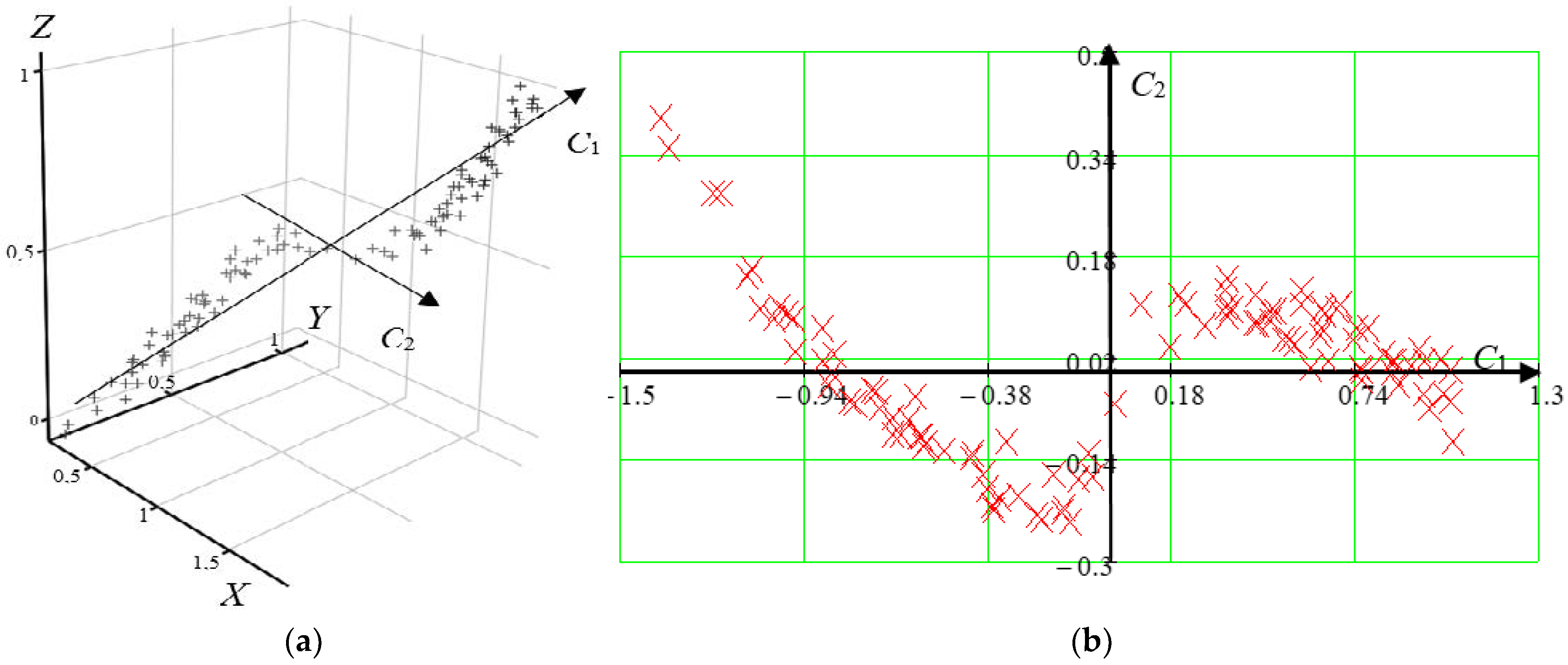
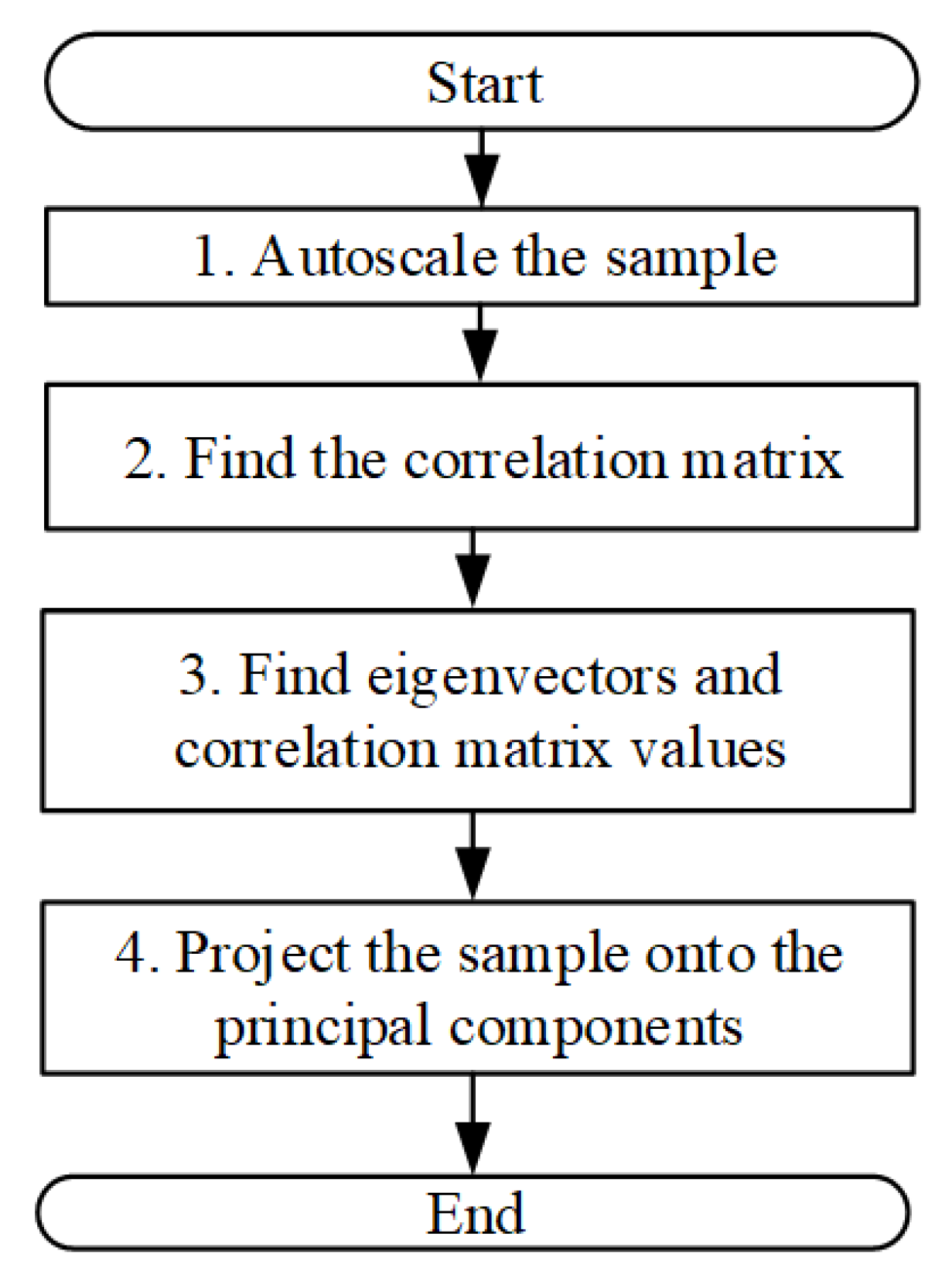
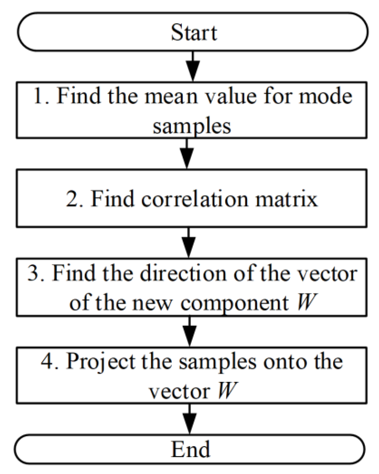
2.1. Implementation of the “Data Compression” Algorithm by Principal Component Analysis Method

One of the options for compressing information and forming generalized features of the relay protection operation is the use of the principal component analysis (PCA) method, also known as the Karhunen–Loev decomposition. This is one of the methods for reducing the dimension of the feature space, which is used in recognition and regression issues [41,42,43,44,45].
The essence of the method lies in the fact that in the initial space of features, a hyperplane of lower dimension is allocated from the condition of the minimum error of projecting the points of the original sample onto this hyperplane. It is proved that the resulting hyperplane will have the following property: The dispersion of the projections of the initial sample on the selected hyperplane will be greater than on any other hyperplane of the same dimension. In other words, the PCA method allows the transition from the feature space of a higher dimension to the space of a lower dimension, while preserving the information contained in the original data as much as possible.
Let us consider a point sampling located in three-dimensional space (Figure 5).
Despite the fact that the sample was initially set in three-dimensional space, Figure 5 shows that the points practically lie in the same plane, which means that their description by three coordinates is redundant. The projection of the sample onto the plane specified by the axes C1 and C2 preserves the internal structure of the initial data with minimal losses. However, due to its smaller dimension, it requires less storage space and is easier to analyze using computer technology.
Thus, by combining the available features for measurement into a single multidimensional space and applying the PCA method to it, we can obtain a dataset of a significantly smaller dimension but reflecting the crucial features of the initial sample. Projections onto the axes of the new feature space (principal component axes) can be considered as new, synthetic features. They have a certain information value, different from the information value of the initial values. In the simplest case, the original feature space can be compressed to one-dimensional, that is, to a straight line. The resulting straight line will “penetrate” the initial sample in the direction of maximum variance.
The Karhunen–Loev transformation is appropriate for use in recognition problems, since it allows one to abandon complex multidimensional classification algorithms and introduce a single generalized feature or feature space that has a significantly lower dimension than the initial training set.
Let us illustrate the application of the PCA method on the following simple example. Let it be necessary to build a one-dimensional classifier that separates two sets of vectors belonging to the classes α and β in the three-dimensional feature space defined by the X, Y, and Z axes. In this case, the features of each class are random variables independent of each other. They are evenly distributed within the given ranges. The distribution ranges of values are given in Table 2.
The location of the points of the training sample in the three-dimensional space of features is shown in Figure 6a. Figure 6b shows a distribution histogram of the sample points projection on the X-axis, and a similar histogram is typical for the other two axes.
If we use projections of sample points on any of the X, Y, or Z-axes as a sign for the functioning of the classifier, then it is possible to accurately classify no more than 90% of the training sample size. Thus, the recognition error will be about 10%.
Let us determine the dispersion D of the distribution of features along the initial axes by Equation (1):
D = 1 N n = 1 N ( a n a ¯ ) 2 ,
where N is the total size of the training sample, which includes classes α and β, an is the projection of the current selection element onto the given axis, and a ¯ is the mathematical expectation of the sample projections on a given axis.
For the example under consideration, the dispersion of the distribution of features along the axes take the following values:
D x = D y = D z = 0.61
Figure 6 shows that the projection of the training sample points onto a straight line passing through the origin at an angle of 45° to each of the X, Y, and Z axes gives the maximum dispersion. Indeed, the calculation shows that the dispersion in the case under consideration is 0.94. Let us construct histograms of the distribution of the training sample projections onto the straight line that specifies the direction of the maximum dispersion (Figure 7). From the analysis of Figure 7, it becomes obvious that the projection under consideration is more informative than the projections on the initial X, Y, and Z axes.
The resulting generalized feature (Figure 7) makes it possible to implement a classifier whose error does not exceed 0.25% of the size of the training sample. The considered example shows that the formation of the initial sample projections on the axes, which provide the greatest dispersion, is expedient for data classification. This allows you to reduce the number of coordinates, while maintaining informativeness. The PCA method is designed to obtain such projections and is applicable for feature space compression [45].
In accordance with this example, it is possible to use only the first principal component and build a one-dimensional relay protection on its basis. Such protection will have the simplest possible implementation, in terms of calculations. It is enough just to compare the linear combination of primary features with the setting.
To find a new feature by the PCA method, it is necessary to perform a number of operations on the training samples that had been obtained earlier (Figure 8).
For autoscaling of the initial sample, it is necessary to perform centering and normalization operations.
The correlation between two random variables is determined by Equation (2):
ρ ( X , Y ) = c o v ( X , Y ) D ( X ) D ( Y )   ,
where cov(X, Y) is the covariance of two random variables X and Y, and D(X), D(Y) is the dispersions of the random variables X and Y, respectively.
A correlation matrix is a matrix that presents the correlation coefficients between features. Its general form is presented in Equation (3):
R x = [ 1 r 12 r 1 k r 21 1 r 2 k r k 1 r k 2 1 ]  
where r is the pairwise correlation coefficients between different k features.
Calculation of eigenvectors and eigenvalues of the correlation matrix is implemented by the rotation method [58]:
  • The initial correlation matrix A is set, and the initial value k = 0 and the error value ℇ > 0 are set.
  • In the upper triangular over-diagonal part of the matrix A, the maximum modulo element aij is singled out.
  • This element is compared with the error value ℇ. If this element is less than the specified error, then the iterative process ends; if it is greater, then the process continues.
  • The angle of rotation is found by Equation (4):
φ ( k ) = 1 2 2 a i j ( k ) a i i ( k ) a j j ( k ) .
5.
The rotation matrix H is compiled.
6.
The next approximation of the matrix A is calculated by Equation (5):
A ( k + 1 ) = ( H ( k ) ) T A ( k ) H ( k ) .
Further, it is necessary to assume that k = k + 1, and proceed to the second point.
After the completion of the iterative process, the main diagonal of the matrix A will contain the eigenvalues of the correlation matrix.
In order to find the eigenvectors, it is necessary to multiply all the rotation matrices H(k). Eigenvectors will be the columns of the matrix obtained as a result of multiplication.
To project the training data onto a new coordinate, the principal component (PC), it is necessary to multiply the autoscaled training sample (B) by the eigenvector of the correlation matrix V1:
P C 1 = B V 1 .
The direction coordinates of such a principal component will essentially be weight coefficients. The input values of the samples are multiplied by them, thereby projecting these values onto this new component.
The above algorithm was implemented by programming in the VBA (Visual Basic for Applications) environment.

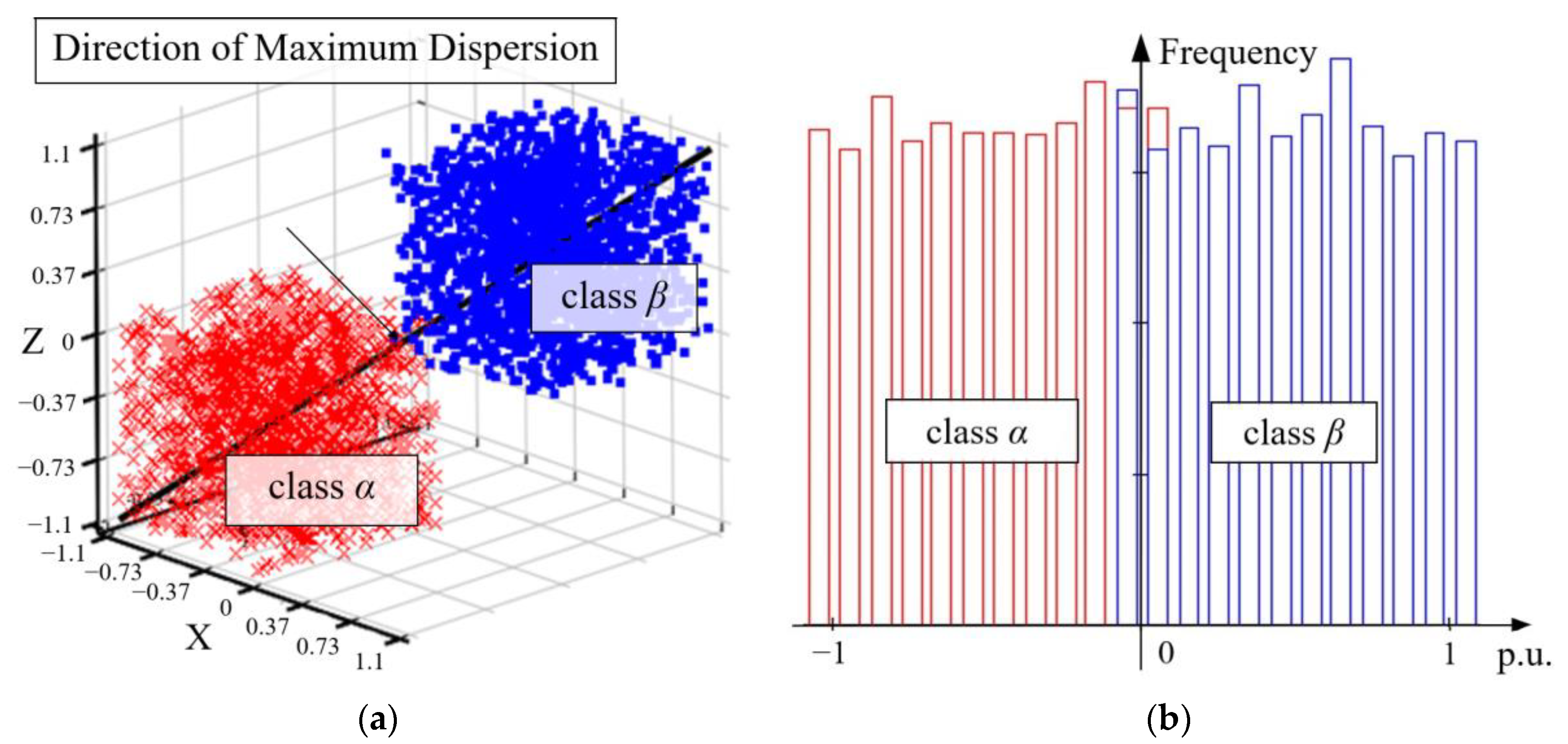
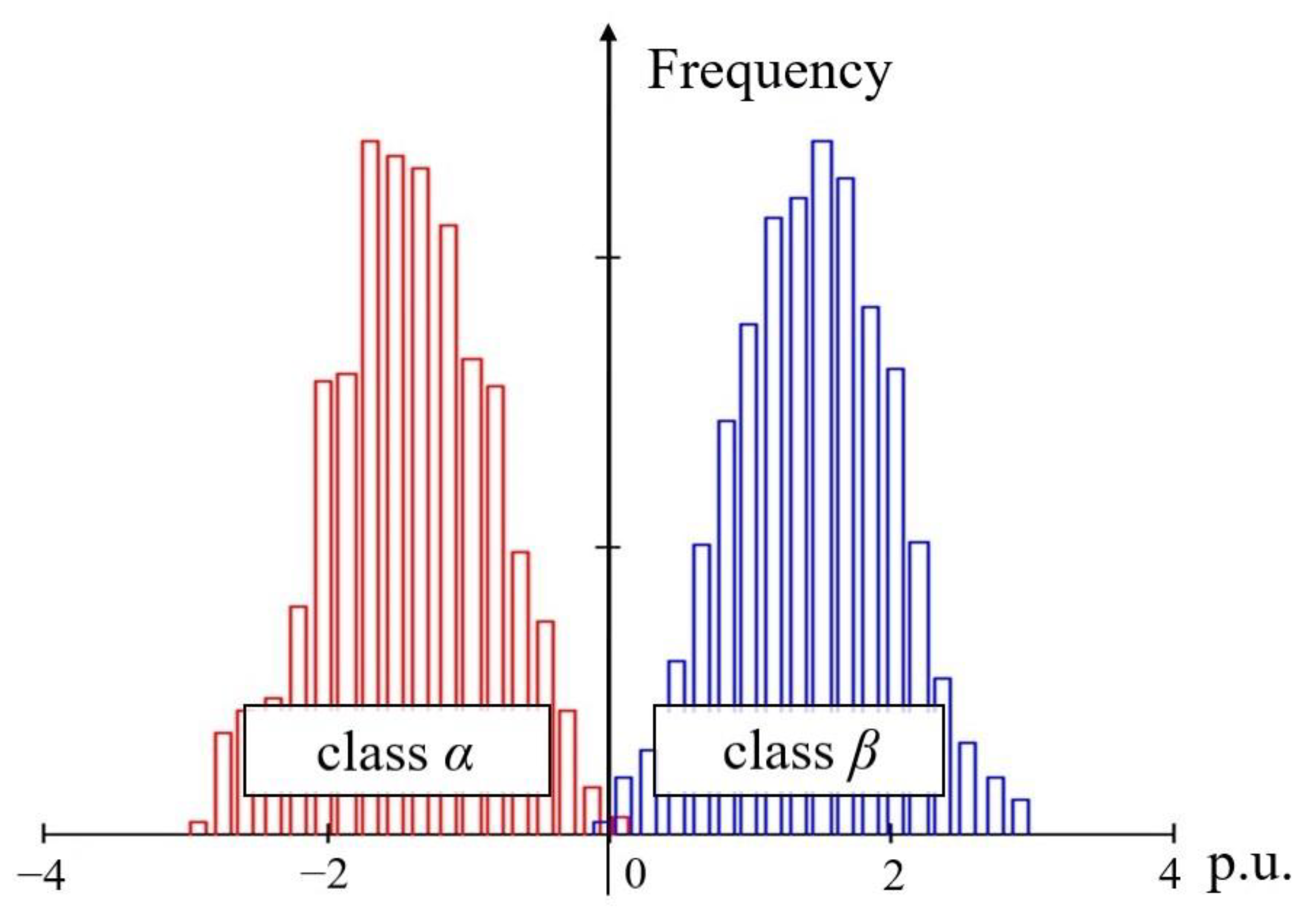
2.2. Implementation of the “Data Compression” Algorithm by the Fisher Linear Discriminant Analysis Method

Similar to the PCA method, linear discriminant analysis (LDA) [39,40,59] makes it possible to single out a subspace of a lower dimension in the initial feature space.
In order to try to separate two samples based on a linear discriminant, an additional criterion is used—the Fisher criterion. Thus, the linear discriminant analysis turns into essentially Fisher’s linear discriminant (FLD).
This method is based on the following conditions:
  • Maximizing the distance between the means of training samples;
  • Minimization of the dispersion within each sample.
The last principle allows you to minimize the overlap of classes.
Suppose we have a set of n d-dimensional samples x1, …, xn, n1 in the subset X1 and n2 in the subset X2. Let us form a linear combination of the components of the vector X and obtain a scalar value:
y = W t X .
Let us introduce the corresponding set n of samples y1, …, yn, divided into subsets Y1 and Y2. If ||W|| = 1, then each component yi is the projection of the corresponding xi onto the line in the direction W.
In this case, FLD is defined as such a linear separating function WtX for which the function is maximum [33]:
J ( W ) = ( m 2 m 1 ) 2 s 1 2 + s 2 2
where m2 and m1, the averages for projected points samples on the resulting axis; s 1 2 and s 2 2 are the scatter for each of the samples. This is an analogue of the dispersion within the sample. That is, the larger it is, the more scattered are the values in this sample.
To obtain J as an explicit function of W, we define the scatter matrices Si and SW by:
S i = x X i ( x m i ) ( x m i ) t .
and
S W = S 1 + S 2 .
Then,
S i 2 = x X i ( W t x W t m i ) 2 = x X i W t ( x m i ) ( x m i ) t W = W t S i W ,
So,
S 1 2 + S 2 2 = W t S W W .
The SW matrix is called the intra-class scatter matrix. It is proportional to the sample covariance matrix for the d-dimensional dataset. It will be symmetric, positive semi-definite, and as a rule, non-degenerate if n > d.
Based on the criterion presented above (Equation (8)), the Fisher linear discriminant is determined. The direction of the new W component onto which the samples are projected maximizes the J(W) function. In the W direction, the projections of the initial samples x1, …, xn are maximally removed from each other.
Fisher determined that the function J(W) reaches its maximum value at:
W = S W 1 ( m 1 m 2 )
where S W 1 is the inverted, averaged scatter matrix within the class.
Thus, applying this method on the sample presented above, we obtain the following result, which is shown in Figure 9. Areas of emergency modes of features x1 and x2 and their linear combination according to the FLD method are shown in red. Areas of normal modes of features x1 and x2 and their linear combination according to the FLD method are shown in blue.
As can be seen from Figure 9, the two-sample data become completely separable. In this case, only one component is used. That is, in this particular case, using FLD, it was possible to reduce the number of components (features), while not losing the information content.
To solve the problem of finding a new feature for recognizing the relay protection mode using the FLD method, it is necessary to perform a number of operations on the training samples obtained earlier (Figure 10).
To find the average values of the training samples, we use Equations (14) and (15):
m 1 = 1 n 1 i = 1 n 1 x i ( 1 ) ,
m 2 = 1 n 2 i = 1 n 2 x i ( 2 ) .
Next, you should find the correlation matrices for the samples corresponding to the normal and emergency modes.
Let us form the internal scatter matrices of data in the sample and find the value for each pair of features according to Equation (9).
The next step is to find the overall matrix by adding the internal scatter matrices.
Next, the direction of the vector W is calculated using Equation (13).
The last operation is to project the sample onto the new resulting vector. This happens by multiplying the initial features by weight coefficients and subsequent addition (Equation (7)). The weight coefficients correspond to the values of the coordinates of the vector W direction.

3. Results

As a result of the algorithm based on the PCA method, orthogonal vectors were obtained that indicate the direction of new features. Thus, having projected the training samples onto the obtained new feature, we obtain two samples located in the new coordinate plane. To demonstrate the results, we present them in the form of graphs and distribution diagrams (Figure 11 and Figure 12).
The following initial features were used: increment of active (∆Ia) and reactive current (∆Ir), negative sequence current (I2), phase value (φ), and active (R) and reactive (X) resistance. Table 3 shows the weight coefficients (K1–K6) for each information feature obtained from the results of a preliminary multiple simulation of modes in the section of the 110/10 kV electrical network (Figure 1) and the use of the PCA method. These weight coefficients are the direction coordinates of the principal component. The initial values of information features are multiplied by the obtained weight coefficients, and thus, these values are projected onto a new component.
Based on the analysis of the obtained graphs, it was found that the use of the most severe case to determine the parameters and coefficients has a positive effect on the recognition of modes. As the most severe mode, a short circuit behind the transformer (110/10 kV, Snom = 6.3 MVA), SS-2 was considered (Figure 1). The samples excluded from training and projected onto the newly obtained vector do not negatively affect the recognition in any way, since they are far from the dividing line of the two samples.
Displaying the results of the FLD algorithm is similar to the PCA algorithm (Figure 13 and Figure 14). It should be noted that in the process of calculations it was found that the most effective initial parameters taken for calculating a new component are: an active and a reactive current increment (∆Ia and ∆Ir), a negative sequence current (I2), a positive sequence current (I1), and an active and a reactive resistance (R and X).
Table 4 shows the weight coefficients (K1-K6) obtained by the FLD method by preliminary simulation similar to the PCA.
It can be seen from the graphs (Figure 13 and Figure 14) that the separation of the two modes of network operation is also achieved. However, a distinctive feature of this approach and the use of FLD as a method of “data compression” is that for training it is necessary to use the most boundary situations. That is, use the most severe case to recognize.

4. Discussion

Various network configuration options were used to estimate the efficiency of the proposed methods. As a result, object characteristics were built [60,61]. They represent the dependence of the limiting transient resistance (RT) at the fault location (at which the protection will be able to recognize the emergency mode) on the remoteness of the fault location from the protection installation site (f(z)) (Figure 15).
Current protections based on full current (I) and reactive current (Ir) were considered when comparing protections that use only one feature to recognize emergency modes. It is clearly seen that the new features obtained by the PCA and LDF methods are many times greater than all the presented features, which could be used to recognize modes. This occurs with a significant removal of the short circuit location. They provide recognition of a short circuit in relation to the normal mode in conditions exceeding 5–6 times the transient resistance.
To demonstrate the possibility of using generalized features when recognizing emergency modes by long-range redundancy relay protection, it is necessary to implement such algorithms on the basis of commercially available relay protection devices [62,63,64].
LRP is the most common means of redundant protection in a low, medium, and high voltage network. It is implemented as a separate function and is usually built using a simple overcurrent protection.
Figure 16 and Figure 17 present variants of the circuits of triggering elements for the LRP based on the PCA method (Figure 16) and FLD method (Figure 17).
In Figure 16, ∆Ia is the active current increment, ∆Ir is the reactive current increment, I2 is the negative sequence current, φ is the phase value, R is the active resistance, X is the reactance, K1–K6 are weight coefficients for each initial feature, and μ is the generalized feature.
In Figure 17, ∆Ia is the active current increment, ∆Ir is the reactive current increment, I2 is the negative sequence current, I1 is the positive sequence current, R is the active resistance, X is the reactance, K1–K6 are the weight coefficients for each initial feature, and μ is the generalized feature.
Structural schemes of the triggering elements of the considered methods are similar and provide for two types of settings [65,66]. The first type of setting is used to obtain a generalized feature μ by weighted summation. This involves multiplying each initial feature by its pre-obtained weight coefficients and summing up with each other. The second type of setting is used to make a decision on the operation of relay protection by comparing the generated generalized feature with the setting. This happens on the principle of simple current protection. At the output of the triggering element, a binary signal is generated for launch (“1”) or not launch (“0”) of the relay protection.
Additionally, in the PCA method, advance autoscaling is applied to its own parameters (Figure 16). This involves subtracting the mean value of the calculated sample from each initial feature and dividing by the mean square value of the calculated sample. In other words, all parameters are reduced to normalized values by the reduction to zero mathematical expectation (mi = 0) and unit dispersion (Di = 1).
The frequency of updating the value in the triggering element is equal to the sampling rate of the RP terminal.
Triggering of the LRP leads to shutdown of the circuit breaker on the protected line, as well as the appearance of the corresponding indication on the RPA terminal [67,68].
In the case of the reconstruction of the electrical network (for example, a change in the composition of consumers, the addition of new power lines, and the emergence of new energy sources), the repeated simulation will be required to form new settings of the first and second types and correct them in the RPA terminal [69,70].
It should be noted that the work of the proposed algorithms is not provided in the “online” mode, which requires a significant computational load on the processor. All calculations are carried out in advance with the receipt of the first type settings and the second type setting in the “offline” mode on specialized software for multiple simulation.
The implementation of the proposed algorithms will not require a significant change in the hardware of the RPA devices. Only a slight modification of the existing software of the device used in operation is required.

5. Conclusions

This article presents examples of the implementation the methods of “data compression” (principal component analysis, Fisher’s linear discriminant analysis) for the transition to a generalized feature of the multi-parameter relay protection, which increases the recognition of electrical network modes.
A PSCAD simulation model has been developed that allows generating statistical data for finding weight coefficients in the multi-parameter relay protection using generalized features.
Long-range redundancy protection using a generalized feature is more effective in recognizing emergency modes (by 5–6 times) than classical protections using a single feature.
The proposed options for the use of generalized features for relay protection-triggering elements can be implemented in modern relay protection and automation terminals without a significant upgrade of their hardware and software.

Author Contributions

Conceptualization, A.K. and A.L.; methodology, P.I.; software, A.L.; validation, A.K., P.I., and A.L.; formal analysis, A.K.; investigation, A.L.; resources, P.I.; data curation, P.I.; writing—original draft preparation, A.L.; writing—review and editing, A.K. and P.I; visualization, A.L. and P.I; supervision, A.K.; project administration, P.I.; funding acquisition, A.L. All authors have read and agreed to the published version of the manuscript.

Funding

This research received no external funding.

Institutional Review Board Statement

Not applicable.

Informed Consent Statement

Not applicable.

Data Availability Statement

Data sharing not applicable. No new data were created or analyzed in this study. Data sharing is not applicable to this article.

Conflicts of Interest

The funders had no role in the design of the study; in the collection, analyses, or interpretation of data; in the writing of the manuscript, or in the decision to publish the results.

References

  1. Lu, X.; Wang, H.; Liu, H.; Xu, C.; Zhang, L.; Jin, Z. Research on Real-time Reliability of Relay Protection System in Intelligent Substation. J. Phys. Conf. Ser. 2020, 1601, 022007. [Google Scholar] [CrossRef]
  2. Chen, J.; Yue, F.; Zhang, Y. A Design to Improve the Reliability of Relay Protection Control Equipment. In Lecture Notes in Electrical Engineering, Proceedings of the 16th Annual Conference of China Electrotechnical Society, Beijing, China, 24–26 September 2021; Springer: Singapore, 2022; Volume 891, p. 891. [Google Scholar] [CrossRef]
  3. Yang, Y. Automatic Calculation and Simulation of Time-Varying Failure Rate of Digital Relay Protection Device. Math. Probl. Eng. 2022, 16, 1–9. [Google Scholar] [CrossRef]
  4. McCalley, J.; Oluwaseyi, O.; Krishnan, V.; Dai, R.; Singh, C.; Jiang, K. System Protection Schemes: Limitations, Risks, and Management; Report Power Systems Engineering Research Center: Tempe, AZ, USA, 2010. [Google Scholar] [CrossRef]
  5. Ilyushin, P.; Volnyi, V.; Suslov, K.; Filippov, S. Review of Methods for Addressing Challenging Issues in the Operation of Protection Devices in Microgrids with Voltages of up to 1 kV that Integrates Distributed Energy Resources. Energies 2022, 15, 9186. [Google Scholar] [CrossRef]
  6. Chen, Q.; Zhou, X.; Sun, M.; Zhang, X. Fault Tracking Method for Relay Protection Devices. Energies 2021, 14, 2723. [Google Scholar] [CrossRef]
  7. Ghahremani, E.; Heniche-Oussedik, A.; Perron, M.; Racine, M.; Landry, S.; Akremi, H. A Detailed Presentation of an Innovative Local and Wide-Area Special Protection Scheme to Avoid Voltage Collapse: From Proof of Concept to Grid Implementation. IEEE Trans. Smart Grid 2019, 10, 5. [Google Scholar] [CrossRef]
  8. Subkhanverdiev, K.S. Calculation of specific operating modes of relay protection for AC traction networks. Vestn. Railw. Res. Inst. 2020, 79, 245–248. [Google Scholar] [CrossRef]
  9. Zhang, Z.; Kang, Y.; Xie, X. Online Verification method of Relay Protection Settings Based on ETAP software. IOP Conf. Ser. Earth Environ. Sci. 2020, 514, 042060. [Google Scholar] [CrossRef]
  10. Sharygin, M.; Vukolov, V.; Petrov, A. Adaptive multivariable relay protection of reconfigurable distribution networks. In E3S Web Conf. 2019, 139, 01048. [Google Scholar] [CrossRef]
  11. Romanov, Y.V.; Voronov, P.I. Assessing the Sensitivity of Relay Protection. Power Technol. Eng. 2018, 51, 728–731. [Google Scholar] [CrossRef]
  12. Nedelchev, N.; Matsankov, M. Increasing the Sensitivity of the Digital Relay Protection Against Turn-to-turn Short Circuits and Asymmetries in Wind Power Generators. E3S Web Conf. 2020, 186, 03001. [Google Scholar] [CrossRef]
  13. Ilyushin, P.V. Emergency and post-emergency control in the formation of micro-grids. E3S Web Conf. 2017, 25, 02002. [Google Scholar] [CrossRef]
  14. Zhang, J.; Lin, R.; Tao, W. Study of relay protection modeling and simulation on the basis of DIgSILENT. Dianli Xitong Baohu Yu Kongzhi/Power Syst. Prot. Control. 2018, 46, 62–67. [Google Scholar] [CrossRef]
  15. Kurihara, I.; Takehara, A.; Nakachi, Y.; Kato, Y.; Iwabuchi, N. Development of power system reliability analysis program with consideration of system operation. Wiley. Electr. Eng. Jpn. 2005, 153, 4. [Google Scholar] [CrossRef]
  16. Huang, S. Research on Relay Protection Technology Based on Smart Grid. IOP Conf. Ser. Earth Environ. Sci. 2021, 714, 042084. [Google Scholar] [CrossRef]
  17. Kochetov, I.D.; Liamets, Y.Y.; Martynov, M.V.; Maslov, A.N. Individual and Collective Recognition Capability of the Measuring Elements of Relay Protection. Power Technol. Eng. 2020, 53, 772–776. [Google Scholar] [CrossRef]
  18. Nan, D.; Tan, J.; Zhang, L.; Jingus, J.; Wang, C.; Liu, W. Research on the remote automatic test technology of the full link of the substation relay protection fault information system. Energy Rep. 2022, 8, 1370–1380. [Google Scholar] [CrossRef]
  19. Loskutov, A.A.; Pelevin, P.S.; Vukolov, V.Y. Improving the recognition of operating modes in intelligent electrical networks based on machine learning methods. In Proceedings of the E3S Web of Conferences, Kazan, Russia, 21–25 September 2020; Volume 216, p. 1034. [Google Scholar] [CrossRef]
  20. Loskutov, A.A.; Pelevin, P.S.; Mitrovic, M. Development of the logical part of the intellectual multi-parameter relay protection. In Proceedings of the E3S Web of Conferences, Tashkent, Uzbekistan, 23–27 September 2019; Volume 139, p. 1060. [Google Scholar] [CrossRef]
  21. Kulikov, A.; Loskutov, A.; Bezdushniy, D. Relay Protection and Automation Algorithms of Electrical Networks Based on Simulation and Machine Learning Methods. Energies 2022, 15, 6525. [Google Scholar] [CrossRef]
  22. Atat, R.; Liu, L.; Wu, J.; Li, G.; Ye, Y.; Yi, Y. Big Data Meet Cyber-Physical Systems: A Panoramic Survey. IEEE Access 2018, 6, 73603–73636. [Google Scholar] [CrossRef]
  23. Sharma, M.; Rajpurohit, B.S.; Agnihotri, S.; Singh, S.N. Data Analytics Based Power Quality Investigations in Emerging Electric Power System Using Sparse Decomposition. IEEE Trans. Power Deliv. 2022, 37, 4838–4847. [Google Scholar] [CrossRef]
  24. Wang, Y.; Chen, Q.; Hong, T.; Kang, C. Review of Smart Meter Data Analytics: Applications, Methodologies, and Challenges. IEEE Trans. Smart Grid 2019, 10, 3125–3148. [Google Scholar] [CrossRef]
  25. Ivanov, I.Y.; Novokreshchenov, V.V.; Ivanova, V.R. Current state of the problems of functioning of relay protection and automation complexes used in an active adaptive network. Power Eng. Res. Equip. Technol. 2023, 24, 102–123. [Google Scholar] [CrossRef]
  26. Rylov, A.; Ilyushin, P.; Kulikov, A.; Suslov, K. Testing Photovoltaic Power Plants for Participation in General Primary Frequency Control under Various Topology and Operating Conditions. Energies 2021, 14, 5179. [Google Scholar] [CrossRef]
  27. Wang, Q. Feeder segment switch-based relay protection for a multilayer differential defense-oriented distribution network. Soft Comput. 2022, 26, 4895–4904. [Google Scholar] [CrossRef]
  28. Ilyushin, P.; Filippov, S.; Kulikov, A.; Suslov, K.; Karamov, D. Specific Features of Operation of Distributed Generation Facilities Based on Gas Reciprocating Units in Internal Power Systems of Industrial Entities. Machines 2022, 10, 693. [Google Scholar] [CrossRef]
  29. Tiwari, S.; Jain, A.; Ahmed, N.; Lulwah, C.; Alkwai, M.; Dafhalla, A.; Hamad, S. Machine learning-based model for prediction of power consumption in smart grid- smart way towards smart city. Expert Syst. 2021, 39, 5. [Google Scholar] [CrossRef]
  30. Xu, Y.; Shen, N.; Zhu, X.; Han, D. Equivalent model of DFIG for relay protection setting calculation. Dianli Xitong Baohu Yu Kongzhi/Power Syst. Prot. Control. 2018, 46, 114–120. [Google Scholar] [CrossRef]
  31. Ilyushin, P.; Filippov, S.; Kulikov, A.; Suslov, K.; Karamov, D. Intelligent Control of the Energy Storage System for Reliable Operation of Gas-Fired Reciprocating Engine Plants in Systems of Power Supply to Industrial Facilities. Energies 2022, 15, 6333. [Google Scholar] [CrossRef]
  32. Chen, X.; Xiong, X.; Qi, X.; Zheng, C.; Zhong, J. A big data simplification method for evaluation of relay protection operation state. Proc. Chin. Soc. Electr. Eng. 2015, 35, 538–548. [Google Scholar] [CrossRef]
  33. Duda, R.O.; Hart, P.E. Pattern Classification and Scene Analysis, 1st ed.; Wiley: New York, NY, USA, 1973; p. 512. [Google Scholar]
  34. Witten, I.H.; Frank, E. Data Mining: Practical Machine Learning Tools and Techniques, 2nd ed.; Elsevier: Amsterdam, The Netherlands, 2005; p. 525. [Google Scholar]
  35. Michie, D.; Spiegelhalter, D.; Taylor, C. Machine Learning, Neural and Statistical Classification; Ellis Horwood: Bromley, UK, 1994; p. 290. [Google Scholar]
  36. Bishop, C.M. Pattern Recognition and Machine Learning; Springer: Amsterdam, The Netherlands, 2006; p. 738. [Google Scholar]
  37. Jaen-Cuellar, A.Y.; Trejo-Hernández, M.; Osornio-Rios, R.A.; Antonino-Daviu, J.A. Gear Wear Detection Based on Statistic Features and Heuristic Scheme by Using Data Fusion of Current and Vibration Signals. Energies 2023, 16, 948. [Google Scholar] [CrossRef]
  38. Grimm, A.; Schönfeldt, P.; Torio, H.; Klement, P.; Hanke, B.; von Maydell, K.; Agert, C. Deduction of Optimal Control Strategies for a Sector-Coupled District Energy System. Energies 2021, 14, 7257. [Google Scholar] [CrossRef]
  39. Choubineh, A.; Wood, D.; Choubineh, Z. Applying separately cost-sensitive learning and Fisher’s discriminant analysis to address the class imbalance problem: A case study involving a virtual gas pipeline SCADA system. Int. J. Crit. Infrastruct. Prot. 2020, 29, 100357. [Google Scholar] [CrossRef]
  40. Singh, G.; Pal, Y.; Dahiya, A. Classification of Power Quality Disturbances using Linear Discriminant Analysis. Elsevier. Appl. Soft Comput. 2023, 138, 110181. [Google Scholar] [CrossRef]
  41. Divyasri, K.; Bhat, S.S.; Reddy, A. Traveling-wave distance protection using principal component analysis for a doubly fed system with synchronized measurements. In Proceedings of the 2017 International Conference on Power and Embedded Drive Control (ICPEDC), Chennai, India, 16–18 March 2017. [Google Scholar] [CrossRef]
  42. Yang, Q.; Yin, S.; Li, Q.; Li, Y. Analysis of electricity consumption behaviors based on principal component analysis and density peak clustering. Concurr. Comput. Pract. Exp. 2022, 34, 21. [Google Scholar] [CrossRef]
  43. Amaral, T.G.; Pires, V.F.; Pires, A.J. Fault Detection in PV Tracking Systems Using an Image Processing Algorithm Based on PCA. Energies 2021, 14, 7278. [Google Scholar] [CrossRef]
  44. Fukunaga, K. Introduction to Statistical Pattern Recognition, 2nd ed.; Gardners Books: Tulsa, OK, USA, 1990; 591p. [Google Scholar]
  45. Singh, I. Data Mining and Warehousing; Khanna Book Publishing Co., Ltd.: Delhi, India, 2022; p. 442. [Google Scholar]
  46. Wang, J.; Ma, Y.; Liu, M.; Huang, T.; Xin, G.; Zhuang, B. Research on Relay Protection and Security Automatic Equipment Based on the Last Decade of Big Data. J. Phys. Conf. Ser. 2022, 2276, 012024. [Google Scholar] [CrossRef]
  47. Nithya, P.; Vengattaraman, T.; Sathya, M. Survey on Parameters of Data Compression. REST J. Data Anal. Artif. Intell. 2023, 2, 1–7. [Google Scholar] [CrossRef]
  48. Chen, C.; Xi, W.; Cui, Y.; Dong, T.; Zhang, X.; Shang, W.; Li, N.; Qin, C.; Zhao, Y. Compression algorithm for relay protection equipment data. In Proceedings of the 2019 IEEE 3rd Conference on Energy Internet and Energy System Integration (EI2), Changsha, China, 8–10 November 2019; pp. 1803–1806. [Google Scholar] [CrossRef]
  49. Kucuk, S.; Ajder, A. Analytical voltage drop calculations during direct on-line motor starting: Solutions for industrial plants. Ain Shams Eng. J. 2022, 13, 101671. [Google Scholar] [CrossRef]
  50. Filippov, S.P.; Dilman, M.D.; Ilyushin, P.V. Distributed Generation of Electricity and Sustainable Regional Growth. Therm. Eng. 2019, 66, 869–880. [Google Scholar] [CrossRef]
  51. Aree, P. Dynamic performance of self-excited induction generator with electronic load controller under starting of induction motor load. In Proceedings of the 5th International Conference on Electrical, Electronics and Information Engineering (ICEEIE), Malang, Indonesia, 6–8 October 2017. [Google Scholar] [CrossRef]
  52. Li, X.; Zhang, J.; Luo, Q.; Wang, C. Simulation Application and Research of Relay Protection Project under Virtual Reality Technology. IOP Conf. Ser. Earth Environ. Sci. 2020, 514, 042045. [Google Scholar] [CrossRef]
  53. Dementiy, Y.A. Active Learning of Intelligent Relay Protection: Opposing Modes. Power Technol. Eng. 2022, 55, 939–946. [Google Scholar] [CrossRef]
  54. Ying, L.; Jia, Y.; Li, W. Research on State Evaluation and Risk Assessment for Relay Protection System Based on Machine Learning Algorithm. IET Gener. Transm. Distrib. 2020, 14, 3619–3629. [Google Scholar] [CrossRef]
  55. Stepanova, D.A.; Antonov, V.I.; Naumov, V.A. Compression of the Training Sample of the Smart Protection Device without Compromising its Information Capacity. In Proceedings of the International Ural Conference on Electrical Power Engineering (UralCon), Magnitogorsk, Russia, 24–26 September 2021. [Google Scholar] [CrossRef]
  56. Ilyushin, P.V.; Filippov, S.P. Under-frequency load shedding strategies for power districts with distributed generation. In Proceedings of the 2019 International Conference on Industrial Engineering, Applications and Manufacturing (ICIEAM), Sochi, Russia, 25–29 March 2019. [Google Scholar] [CrossRef]
  57. Ilyushin, P.V.; Pazderin, A.V. Requirements for power stations islanding automation an influence of power grid parameters and loads. In Proceedings of the 2018 International Conference on Industrial Engineering, Applications and Manufacturing (ICIEAM), Moscow, Russia, 15–18 May 2018. [Google Scholar]
  58. Matrices and Eigenvectors. Available online: http://www.casaxps.com/help_manual/mathematics/Matrices_and_EigenvectorsRev6.pdf (accessed on 29 January 2023).
  59. Hastie, T.; Tibshirani, R.; Friedman, J. The Elements of Statistical Learning; Springer Series in Statistics; Springer: New York, NY, USA, 2017. [Google Scholar]
  60. Lyamets, Y.Y.; Antonov, V.I.; Nudelman, G.S. Method of object characteristics for analysis and synthesis of distance protection. Electromechanics 1999, 1, 95. (In Russian) [Google Scholar]
  61. Lyamets, Y.Y.; Nikolaeva, N.V.; Pavlov, A.O. Object characteristics of remote protection. In Proceedings of the 2nd All-Russia Sci.-Tech. Conf. on Information Technologies in Electrical Engineering and Electric Power Industry, Cheboksary, Russia, 4–5 June 1998; Chuvash State University: Cheboksary, Russia, 1998; pp. 141–144. (In Russian). [Google Scholar]
  62. Summers, A.; Patel, T.; Matthews, R.; Reno, M.J. Prediction of Relay Settings in an Adaptive Protection System. 2022 IEEE Power & Energy Society Innovative Smart Grid Technologies Conference (ISGT), New Orleans, LA, USA, 24–28 April 2022; pp. 1–5. [Google Scholar] [CrossRef]
  63. Abbaspour, E.; Fani, B.; Heydarian-Forushani, E.; Al-Sumaiti, A. A multi-agent based protection in distribution networks including distributed generations. Energy Rep. 2022, 8, 163–174. [Google Scholar] [CrossRef]
  64. Yang, T.; Qian, X.; Ren, L. Application of Artificial Intelligence Algorithm in Relay Protection of Distribution Network. Int. Trans. Electr. Energy Syst. 2022, 2022, 7138367. [Google Scholar] [CrossRef]
  65. Bonetti, A.; Larsson, S.; Schottenius, L.; Wetterstrand, N. Relay protection test challenges in smart grid DER. 2022 IEEE International Conference on Power Systems Technology (POWERCON), Kuala Lumpur, Malaysia, 12–14 September 2022; pp. 1–6. [Google Scholar] [CrossRef]
  66. Doletskaya, L.; Ziryukin, V.; Solopov, R. An electric power system object model creating experience for researching the operation of digital means of relay protection and automation. J. Appl. Inform. 2021, 16, 83–95. [Google Scholar] [CrossRef]
  67. Kulikov, A.; Ilyushin, P.; Loskutov, A.; Suslov, K.; Filippov, S. WSPRT Methods for Improving Power System Automation Devices in the Conditions of Distributed Generation Sources Operation. Energies 2022, 15, 8448. [Google Scholar] [CrossRef]
  68. Hao, G.; Lin, Z.; Wu, X.; Chen, X. The Comprehensive Recognition Method of Critical Lines Based on the Principal Component Analysis. J. Electr. Eng. Technol. 2023, 1–10. [Google Scholar] [CrossRef]
  69. Andreev, M.V. Investigation of Processes in the Measuring Part of Digital Devices of Relay Protection in the MATLAB Software Package. Russ. Electr. Eng. 2019, 90, 530–537. [Google Scholar] [CrossRef]
  70. Andreev, M.; Suvorov, A.; Askarov, A.; Rudnik, V.; Bhalja, B.R. Novel Approach for Relays Tuning Using Detailed Mathematical Model of Electric Power System. Int. J. Electr. Power Energy Syst. 2022, 135, 107572. [Google Scholar] [CrossRef]
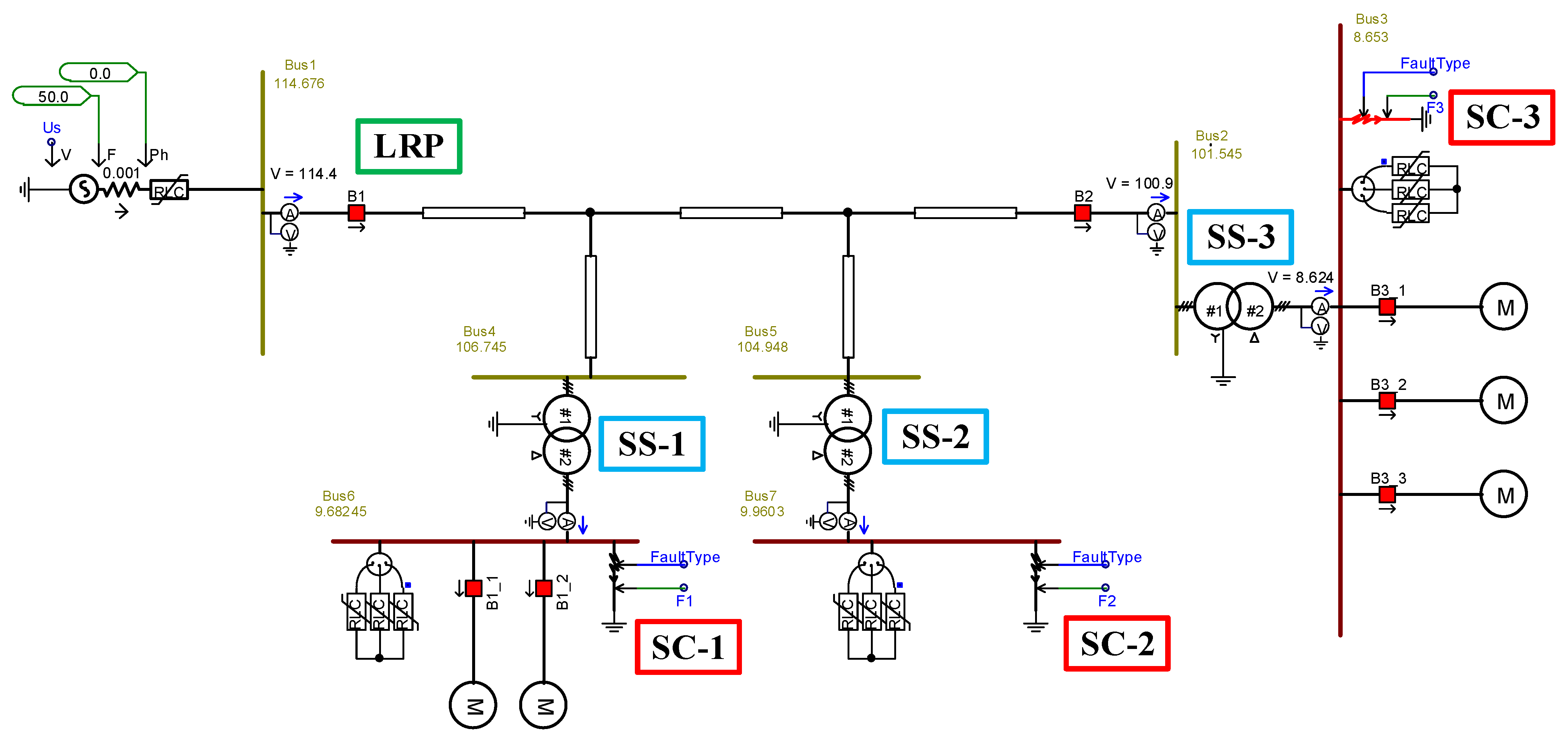
Figure 1. PSCAD model of a 110/10 kV network section (LRP – long-range redundancy protection; SS-1, SS-2, SS-3—substations; SC-1, SC-2, SC-3—short-circuit currents points).
Information 14 00230 g001
Figure 2. Distribution of total currents in normal and emergency modes.
Information 14 00230 g002
Figure 3. Distribution of reactive currents in normal and emergency modes.
Information 14 00230 g003
Figure 4. Active resistances and reactances.
Information 14 00230 g004
Figure 5. Graphical representation of a point sampling: (a) point sampling in three-dimensional space; (b) projection of the initial sample onto the plane C1-C2 (C1-C2—the first and second components).
Information 14 00230 g005
Figure 6. Distribution of feature values: (a) position of points in three-dimensional space; (b) histogram of the distribution of feature projections on the X-axis.
Information 14 00230 g006
Figure 7. Distribution of training sample points projections on the direction of maximum dispersion.
Information 14 00230 g007
Figure 8. Principal component learning algorithm.
Information 14 00230 g008
Figure 9. Projected samples on the component obtained using the Fisher criterion.
Information 14 00230 g009
Figure 10. Fisher’s linear discriminant learning algorithm.
Information 14 00230 g010
Figure 11. Full emergency sampling for the first principal component (PC1).
Information 14 00230 g011
Figure 12. The most severe emergency sampling for the second principal component (PC2).
Information 14 00230 g012
Figure 13. Full emergency sampling for the FLD component.
Information 14 00230 g013
Figure 14. The most severe emergency sampling for the FLD component.
Information 14 00230 g014
Figure 15. Object characteristic.
Information 14 00230 g015
Figure 16. Scheme of the triggering element based on the PCA method.
Information 14 00230 g016
Figure 17. Scheme of the triggering element based on the FLD method.
Information 14 00230 g017
Table 1. Randomly changing parameters of the PSCAD model.
ParameterChange Range
System Voltage[0.95… 1.05] p.u.
System impedance modulus[6… 12] Ohm
System resistance angle[80… 90] deg.
Line resistance[0.95… 1.05] p.u.
Load value SS-1Active load power[9… 36] kW
tgφ[0.2… 0.6] p.u.
Load value SS-2Active load power[1.2… 6] kW
tgφ[0.2… 0.6] p.u.
Load value SS-3Active load power[5… 18] kW
tgφ[0.2… 0.6] p.u.
For short circuitsTransient resistance[0… 5] Ohm
Type of short circuitABC; AB; BC; CA
Table 2. Distribution ranges of features in the training sample.
FeatureClass αClass β
X−1.1… 0.1−0.1… 1.1
Y−1.1… 0.1−0.1… 1.1
Z−1.1… 0.1−0.1… 1.1
Table 3. Output values of the weight coefficients of the PCA algorithm.
TrainingWeight Coefficients
K1K2K3K4K5K6
Initial features ΔIa ΔIrRXI2φ
Full emergency sample−0.5470.534−0.4410.454−0.0751
Most severe emergency sample−0.754−0.707−0.746−0.9421−0.037
Table 4. Output values of the weight coefficients of the FLD algorithm.
TrainingWeight Coefficients
K1K2K3K4K5K6
Initial features ΔIa ΔIrRXI2I1
Full emergency sample0.469−0.351−0.0006−0.0017510.485
Most severe emergency sample0.83810.00014−0.00150.186−0.159
Disclaimer/Publisher’s Note: The statements, opinions and data contained in all publications are solely those of the individual author(s) and contributor(s) and not of MDPI and/or the editor(s). MDPI and/or the editor(s) disclaim responsibility for any injury to people or property resulting from any ideas, methods, instructions or products referred to in the content.

