Adaptive Kernel Graph Nonnegative Matrix Factorization

Abstract

Nonnegative matrix factorization (NMF) is an efficient method for feature learning in the field of machine learning and data mining. To investigate the nonlinear characteristics of datasets, kernel-method-based NMF (KNMF) and its graph-regularized extensions have received much attention from various researchers due to their promising performance. However, the graph similarity matrix of the existing methods is often predefined in the original space of data and kept unchanged during the matrix-factorization procedure, which leads to non-optimal graphs. To address these problems, we propose a kernel-graph-learning-based, nonlinear, nonnegative matrix-factorization method in this paper, termed adaptive kernel graph nonnegative matrix factorization (AKGNMF). In order to automatically capture the manifold structure of the data on the nonlinear feature space, AKGNMF learned an adaptive similarity graph. We formulated a unified objective function, in which global similarity graph learning is optimized jointly with the matrix decomposition process. A local graph Laplacian is further imposed on the learned feature subspace representation. The proposed method relies on both the factorization that respects geometric structure and the mapped high-dimensional subspace feature representations. In addition, an efficient iterative solution was derived to update all variables in the resultant objective problem in turn. Experiments on the synthetic dataset visually demonstrate the ability of AKGNMF to separate the nonlinear dataset with high clustering accuracy. Experiments on real-world datasets verified the effectiveness of AKGNMF in three aspects, including clustering performance, parameter sensitivity and convergence. Comprehensive experimental findings indicate that, compared with various classic methods and the state-of-the-art methods, the proposed AKGNMF algorithm demonstrated effectiveness and superiority.

1. Introduction

In pattern recognition, machine learning and data mining, clustering can help to decipher the data distribution and cluster data characteristics. The key point of clustering tasks is to find the internal structure information of the original data and make them more discriminative [1,2,3,4]. Several methods have been developed for clustering, including spectral clustering and k-means [5,6,7], which rely on the metric of data similarity [8,9,10]. Due to the potential clustering representation, nonnegative matrix factorization, which is an effective method for data dimensionality reduction and feature extraction, has been widely used in clustering tasks [11,12]. NMF expresses part-based data by finding two nonnegative matrices whose product is close to the raw data and only allows additive combinations of data. Differently from the interpretability limitations of other matrix-factorization methods involving singular value decomposition (SVD) [13], independent component analysis (ICA) [14], principal component analysis (PCA) [15], etc., with a negative decomposition component, NMF can provide the nonnegative factorization of multivariate data [16,17]. NMF also offers ease of implementation and decomposition, and the interpretability of factorization results.

Many studies show that real-world data can be considered as representations from a nonlinear low-dimensional manifold [18,19,20]. Ordinary NMF [21] ignores the intrinsic manifold structure of the data space. Therefore, Cai et al. [22] proposed graph regularization NMF (GNMF) to explore the geometric relationship of the data as a graph-regularization method for improving the performance of clustering. However, GNMF is a linear method that fails to exploit the nonlinear characteristics of the data. In the work of Tolić et al. [23], the nonlinear graph-regularized KNMF (KOGNMF) was further proposed, where the nonlinear properties of the manifold and its global geometric structure are induced. However, the graph adjacency matrix employed in the KOGNMF is predefined by the k-nearest-neighborhood (knn) or $ϵ$ ball graph technique. The graph constructed by these methods is sensitive to noise and outliers in the data [24,25,26]. In order to overcome this drawback, a learning method is utilized to generate the graph similarity matrix and then regularize the NMF method [27]. Nevertheless, graph learning and matrix factorization are still performed as two separate steps, which leads to suboptimal performance for clustering.

Recently, Peng et al. [28] proposed a flexible NMF with adaptively learned graph regularization (FNMFG), where the graph is jointly learned with matrix factorization. Analogously, the adaptive graph-regularized NMF (NMFAN) method was proposed [29]. Yi et al. [30] proposed the NMF with locality constrained adaptive graph (NMF-LCAG), which can integrate nonnegative matrix factorization and adaptive graph learning with two locality constraints. Instead of predefined graph-based manifold regularization terms, the unified formulations can simultaneously optimize the similarity matrix and the data representation, resulting in better performance. To avoid situations where the non-convexity of NMF models frequently reaches poor local solutions in the presence of noise or outliers, Chen et al. [31] proposed sparsity-constrained graph non-negative matrix factorization (SGNMF) to enhance robustness and eliminate noise, and sparse graph non-negative matrix factorization was presented as a global optimization problem by applying the sum of the different smooth functions to approximate the ${\mathbf{l}}_0$ norm. Yang et al. [32] proposed self-paced nonnegative matrix factorization with adaptive neighbors (SPLNMFAN). Self-paced regularization is introduced to find a better factorized matrix by sequentially selecting data, and the adaptive graph learns the data graph by selecting the local optimal neighbors for each data point. However, since the existing graph-based NMF models are essentially linear, they are not suitable for tasks that deal with nonlinear data.

In this paper, we propose a novel, graph-regularized NMF model referred to as the adaptive kernel graph nonnegative matrix factorization (AKGNMF) model to overcome the above limitations from a new point of view and explore the manifold structure on nonlinear subspaces by adaptively learning the kernel similarity of high-dimensional mappings. Compared with traditional nonnegative matrix-factorization methods, AKGNMF maps origin data to high-dimensional subspaces and learns global similarity through adaptive graphs, further introducing a flexible graph regularization item that preserves local manifold structures. This strategy is able to exploit nonlinear structural information and obtain factorizations with efficient feature representations. In order to mine the potential structural information of nonlinear data, we used the idea of subspace clustering based on Gaussian kernels to project the original data. Specifically, we tried to acquire the global kernel similarity between the original high-dimensional feature space and the mapped subspace; decomposed the sample matrix of the nonlinear mapping to obtain the feature matrix and coefficient matrix; and used the manifold structure obtained by adaptive learning to constrain it to obtain the features under the high-dimensional nonlinear space. Importantly, we presented a unified framework for graph learning and matrix factorization simultaneously. The learned graph was optimized by combining the kernel matrix and the coefficient matrix to alternate iterations jointly, so that the global structure information of the similarity matrix and the local topology of the coefficient representation can be used simultaneously. During the learning procedure, the factorization matrix and the similarity matrix negotiate with each other to find the optimal subspace that maintains the original structure information to the greatest extent. Moreover, an efficient iterative solution was derived to optimize our problem. The convergence of the solution is also demonstrated. The major contributions are summarized as follows:

(1)

We performed learning using an optimal graph that most closely approximates the initial kernel matrix, and attempted to preserve the sample’s similarity. This adaptive strategy can better accomplish manifold structure learning.

(2)

Both the similarity matrix of graphs and the decomposition matrix from the high-dimensional nonlinear mapping features of the original data can be learned in the proposed model. All variables are reciprocally updated in an alternating iterative optimization algorithm, and we simultaneously obtained similarity information and valid feature representation.

(3)

Our method takes non-linear mapping into consideration, meaning it is more capable of handling both linear and non-linear data. Instead of using the previous constructed and fixed graph-regularization term, the adaptively learned similarity preserves the ideal local geometry structure for feature representation. Moreover, the kernel matrix itself contains global similarity information of data points; hence, it is feasible to conserve the overall relations by learning the graph close to the kernel.

(4)

Comprehensive experiments were conducted on both synthetic and real-world datasets to exhibit the effectiveness of the proposed algorithms and demonstrate their superiority.

AKGNMF has potential application value in real-world scenarios such as face recognition, speech recognition, and biomedical engineering. From the perspective of pattern recognition, NMF is essentially a method of dimensionality reduction and feature extraction. For the feature extraction of a face or a voice, the aim is to obtain a matrix-factorization method with sparser decomposition results, a greater number of obvious local features, less redundancy between data and a faster decomposition speed. These real-world data are often nonlinear, and AKGNMF can capture the structural information of the data in a high-dimensional space and has the potential to obtain more effective features with higher precision. In addition, to manage the complex data in biomedicine and chemical engineering, AKGNMF can provide efficient and fast preprocessing for the analysis of these data. As the decomposition of NMF does not have negative values, combining the structural information of adaptive learning to analyze the molecular sequence of gene DNA can make the analysis results more reliable.

The rest of this paper is organized as follows: In Section 2, we briefly introduce NMF, GNMF and similarity-preserving clustering for graph learning. In Section 3, we propose the AKGNMF model framework and algorithm and discuss solutions. Section 4 introduces the comparison and initial analysis of the experimental results of our method and other nonnegative factorization clustering methods on seven datasets. Finally, conclusions are provided in Section 5.

2. Related Work

In this work, all vectors are denoted with boldface lowercase letters and all matrices are denoted with boldface uppercase letters. The important notation mentioned in the following is summarized in

Table 1. Notation.

Notations	Definition
m	the dimensionality of a dataset
n	the number of data points
c	the number of clusters
$\mathbf{K}\in {\mathbb{R}}_n^n$	the kernel matrix
$\mathbf{X}\in {\mathbb{R}}_m^n$	the input data matrix
$\mathbf{L}\in {\mathbb{R}}_n^n$	the graph Laplacian matrix
$\Phi (·)\in {\mathbb{R}}_D^n$	the nonlinear mapping function
$\mathbf{W}\in {\mathbb{R}}_m^k$	the basis matrix in input space
$\mathbf{H}\in {\mathbb{R}}_n^k$	the cluster indicator matrices
$\mathbf{F}\in {\mathbb{R}}_n^k$	the basis matrix in mapped space
$\mathbf{1}$	the all-one column vector
$\mathbf{I}$	the identity matrix
$\mathbf{S}\in {\mathbb{R}}_n^n$	the similarity matrix
Tr(·)	the trace operator of a matrix
${∥·∥}_F$	the Frobenius norm

.

2.1. Graph-Regularized Nonnegative Matrix Factorization

NMF is a matrix decomposition method under the constraint that all elements in the matrix are nonnegative numbers. The main idea is that for any given nonnegative matrix $\mathbf{X}$, the NMF algorithm can find a nonnegative matrix $\mathbf{W}$ and a nonnegative matrix $\mathbf{H}$, thereby decomposing a nonnegative matrix into the left and right nonnegative matrices. Let $\mathbf{X}=[{\mathbf{x}}_{\mathbf{1}},...,{\mathbf{x}}_{\mathbf{n}}]$ be a matrix with column vectors ${\mathbf{x}}_i\approx {\mathbb{R}}^m$; thus, the NMF problem can be formulated as follows:

$$\mathbf{X}\approx {\mathbf{WH}}^{\top }$$

(1)

where $\mathbf{W}=({\mathbf{w}}_{\mathbf{1}},...,{\mathbf{w}}_{\mathbf{n}})\in {\mathbb{R}}^{m\times k}$ and $\mathbf{H}=({\mathbf{h}}_{\mathbf{1}},...,{\mathbf{h}}_{\mathbf{n}})\in {\mathbb{R}}^{n\times k}$ are two nonnegative matrices, and k is a prespecified rank parameter. The column vectors of $\mathbf{W}$ are called the basis vectors, and the column vectors of $\mathbf{H}$ are called the encoding vectors. Two mechanisms are proposed to estimate the quality of NMF in Equation (1). The former is based on the Euclidean distance, and the latter is based on the divergence distance [33]. In this paper, we focus on the former, and the corresponding objective function can be formulated as follows:

$$\underset{\mathbf{W},\mathbf{H}\ge \mathbf{0}}{min}{∥\mathbf{X}-{\mathbf{WH}}^{\top }∥}_F^2$$

(2)

where $∥·∥$ denotes the Frobenius norm of a matrix.

When being performed within the Euclidean space, the NMF-based method is inappropriate for revealing the intrinsic geometric structure of data space in common cases. Cai et al. [22] proposed a novel graph-regularized nonnegative matrix-factorization algorithm that, in addition to learning a parts-based representation, can also combine a geometric-based regularizer. Thus, the intrinsic geometrical and discriminating structures of the data space are available to be discovered. The GNMF is effective at solving clustering problems, since the intrinsic geometrical structure is revealed by incorporating a Laplacian regularization term.

The GNMF objective function based on Euclidean distance is minimized as follows:

$${\mathcal{O}}_{\mathrm{GNMF}}={\parallel \mathbf{X}-{\mathbf{WH}}^{\top }\parallel }_F^2+\beta Tr\left({\mathbf{H}}^{\top }\mathbf{L}\mathbf{H}\right)$$

(3)

where $\beta >0$ is the regularization parameter, $Tr(·)$ indicates the trace of a matrix and $\mathbf{L}$ is the graph Laplacian which satisfies the equation $\mathbf{L}=\mathbf{D}-\mathbf{W}$, where $\mathbf{D}$ is a diagonal matrix in which the entries are column (or row, since $\mathbf{W}$ is symmetric) sums of $\mathbf{W}$.

The aim of GNMF is to find a parts-based representation space in which two data points are sufficiently close to each other when they are connected in the graph. The geometric information is encoded by constructing a nearest neighbor graph; however, the graph-based methods can be easily affected by the input affinity matrix and use of Laplacian graphs. Namely, these methods are affected by several elements such as the neighborhood size, choices of weighting metric, etc.

2.2. Graph Learning

Recently, graph learning methods, including adaptive local structure learning and adaptive global structure learning techniques, have been proposed to obtain the structural information of the data automatically. To preserve the local manifold structure, adaptive-neighbor-based methods [34,35] have been proposed to obtain an optimal graph of input data in several machine learning tasks.

The self-expression method is a global similarity learning approach in graph learning [36]. It assumes that each data point can be expressed as a linear combination of other data points of the dataset. If data points $x_i$ and $x_j$ are similar to each other, the corresponding weight $z_{ij}$ (and $z_{ji}$) is assigned a larger value. Therefore, Z can be regarded as the similarity matrix, and the self-expression-based graph learning problem can be formulated as follows:

$$\underset{\mathbf{Z}}{min}\frac{1}{2}{\parallel \mathbf{X}-\mathbf{XZ}\parallel }_F^2+\mu \rho \left(\mathbf{Z}\right)s.t.\mathbf{Z}\ge 0$$

(4)

where $\mu >0$ is a trade-off parameter and $\rho \left(\mathbf{Z}\right)$ is a regularizer of $\mathbf{Z}$. Two commonly used assumptions about $\mathbf{Z}$ are low-rank and sparse assumptions, which means the learned $\mathbf{Z}$ can reveal the low-dimensional structure of data and can also be robust to the data scale. Equation (4) can be used to identify the neighbors automatically corresponding to the optimization process and utilizes all data points to capture the global structural information. In this way, the individual pairwise similarity information hidden in the data is explored [34] and the graph similarity matrix can be obtained automatically from data.

The graph learning techniques lead to a better structural representation of data relationships than the traditional method in many tasks of machine learning [8]. However, most existing methods are linear models for original data, which ignore the nonlinear hidden structures in data.

3. Adaptive Kernel Graph Nonnegative Matrix Factorization

In this section, we propose a nonlinear adaptive graph-regularized NMF algorithm that can jointly perform nonnegative matrix factorization with graph-similarity learning in kernel spaces. The nonlinear relationship between input samples is also explored, which promotes the improvement of clustering performance.

3.1. Kernel Nonnegative Matrix Factorization Review

In order to handle nonlinear data, we consider the basic idea of kernel subspace clustering. Then, the data can be mapped into a nonlinear transformation to the higher D-dimensional space by performing kernel tricks. We assume that $\Phi \left(x_i\right)$ represents the subspaces of the kernel space, and let $\mathbf{K}\in {\mathbb{R}}_n^n$ be a kernel matrix whose elements are computed as follows:

$${\mathbf{K}}_{ij}={({\Phi }^{\top }\left(\mathbf{X}\right)\Phi \left(\mathbf{X}\right))}_{ij}={\Phi }^{\top }\left(x_i\right)\Phi \left(x_j\right)=ker(x_i,x_j)$$

(5)

where $ker:{\mathbb{R}}^d\times {\mathbb{R}}^d\to R$ is the kernel function and

$$\Phi \left(\mathbf{X}\right)=[\Phi \left(x_1\right),\Phi \left(x_2\right),...,\Phi \left(x_n\right)].$$

(6)

The nonlinear NMF problem aims to find two nonnegative matrices, $\mathbf{W}$ and $\mathbf{H}$, whose product can be used to approximate the mapping of the original matrix:

$$\begin{array}{c}\hfill \Phi \left(\mathbf{X}\right)\approx {\mathbf{WH}}^{\top }\end{array}$$

(7)

where $\mathbf{W}$ is the basis in feature space and $\mathbf{H}$ is the clustering matrix. As $\Phi$ is derived from the representation of high-dimensional space, it is unreasonable to decompose $\Phi \left(\mathbf{X}\right)$ directly [37,38]. According to [37], we use $\mathbf{W}$ as a linear combination of transformed input data points to solve this problem. Thus, we assume that $\mathbf{W}$ lies in the column space of $\Phi \left(\mathbf{X}\right)$:

$$\mathbf{W}=\Phi \left(\mathbf{X}\right)\mathbf{F}$$

(8)

Equation (2) can be interpreted as a representation of simple conversion to the new basis, and the minimization problem can be generalized as follows:

$$\underset{\mathbf{F},\mathbf{H}\ge 0}{min}{\parallel \Phi \left(\mathbf{X}\right)-\Phi \left(\mathbf{X}\right){\mathbf{FH}}^{\top }\parallel }_F^2.$$

(9)

3.2. Adaptive Kernel Graph Nonnegative Matrix Factorization

To exploit the geometric structure of the data in the nonlinear feature space, the kernel-graph-regularization term is integrated within the KNMF method. As mentioned previously, the NMF aims to identify the best-approximated basis vectors applied to the data $\Phi \left(\mathbf{X}\right)={\mathbf{WH}}^{\top }$. Let ${\mathbf{h}}_i=[h_{i1},...,h_{ik}]$ imply the ith column of $\mathbf{H}$, i.e., the ${\mathbf{h}}_i$ representing the ith data point with respect to the basis $\mathbf{W}=\Phi \left(\mathbf{X}\right)\mathbf{F}$. According to the local invariance assumption of the graph-regularization term [39,40,41], for a data distribution, if there exist two data points $\Phi \left(x_i\right)$ and $\Phi \left(x_j\right)$ with significant similarity in the original geometry, then the low dimensional representations of ${\mathbf{h}}_i$ and ${\mathbf{h}}_j$ can retain the same relationship. This can be measured, as shown below:

$$\begin{array}{cc}\hfill \frac{1}{2}\sum _{i,j=1}^n{∥{\mathbf{h}}_i-{\mathbf{h}}_j∥}_F^2{\mathbf{S}}_{ij}& =\sum _{i=1}^n{\mathbf{h}}_i{\mathbf{h}}_i^{\top }{\mathbf{D}}_{i,i}-\sum _{i,j=1}^n{\mathbf{h}}_i{\mathbf{h}}_j^{\top }{\mathbf{S}}_{i,j}\hfill \\ \hfill & =Tr\left({\mathbf{H}}^{\top }{\mathbf{D}}_{\mathbf{S}}\mathbf{H}\right)-Tr\left({\mathbf{H}}^{\top }\mathbf{S}\mathbf{H}\right)\hfill \\ \hfill & =Tr\left({\mathbf{H}}^{\top }{\mathbf{L}}_{\mathbf{S}}\mathbf{H}\right)\hfill \end{array}$$

(10)

where Laplacian matrix ${\mathbf{L}}_{\mathbf{S}}={\mathbf{D}}_{\mathbf{S}}-\mathbf{S}$, and $\mathbf{S}$ is a symmetric similarity matrix. $\mathbf{S}=\frac{\mathbf{S}+{\mathbf{S}}^{\top }}{2}$. ${\mathbf{D}}_{\mathbf{S}}$ is a diagonal matrix whose elements are the column sums of $\mathbf{S}$. Then, we can obtain the following KNMF model with graph regularization, as follows:

$$\begin{array}{c}\underset{\mathbf{F},\mathbf{H}}{min}{\parallel \Phi \left(\mathbf{X}\right)-\Phi \left(\mathbf{X}\right)\mathbf{F}{\mathbf{H}}^{\top }\parallel }_F^2+\beta Tr\left({\mathbf{H}}^{\top }{\mathbf{L}}_{\mathbf{S}}\mathbf{H}\right)\\ s.t.\mathbf{H}\ge 0,\mathbf{F}\ge 0.\end{array}$$

(11)

The fixed similarity matrix in Equation (11) is predefined by the original input data, which may be sub-optimal for the embedded representation $\mathbf{H}$. We also note that the representation matrix $\mathbf{H}$ is computed from the nonlinear feature space of input data, but the graph is obtained from the original input data space. To exploit the nonlinear graph information of input data in kernel spaces, we induce the self-expression-based, global graph-learning term to solve Equation (11) in the kernel spaces. Then, our objective function is formulated as follows:

$$\begin{array}{c}\underset{\mathbf{H},\mathbf{F},\mathbf{S}}{min}\parallel \Phi \left(\mathbf{X}\right)-\Phi \left(\mathbf{X}\right)\mathbf{F}{\mathbf{H}}^{\top }{\parallel }_F^2+\beta Tr\left({\mathbf{H}}^{\top }{\mathbf{L}}_{\mathbf{S}}\mathbf{H}\right){+\gamma \parallel \Phi \left(\mathbf{X}\right)-\Phi \left(\mathbf{X}\right)\mathbf{S}\parallel }_F^2+\mu {\parallel \mathbf{S}\parallel }_F^2\\ s.t.\mathbf{H}\ge 0,\mathbf{F}\ge 0,\mathbf{S}\ge 0\end{array}$$

(12)

where $\gamma$ is a trade-off parameter. In this way, we unified the graph similarity learning and NMF in nonlinear space. We noticed that the graph similarity in Equation (12) considers both the nonlinear mapping feature $\Phi \left(\mathbf{X}\right)$ and the embedded representation $\mathbf{H}$, which leads to a much more flexible regularization for the first error term. By substituting the quadratic terms with a kernel matrix, Equation (12) can be further transformed to the following formulation:

$$\begin{array}{c}\underset{\mathbf{H},\mathbf{F},\mathbf{S}}{min}Tr\left(\mathbf{K}-2{\mathbf{KFH}}^{\top }+{\mathbf{FH}}^{\top }{\mathbf{KHF}}^{\top }\right)+\beta Tr\left({\mathbf{H}}^{\top }{\mathbf{L}}_{\mathbf{S}}\mathbf{H}\right)+\gamma Tr\left(\mathbf{K}-\mathbf{2}\mathbf{KS}+{\mathbf{S}}^{\top }\mathbf{KS}\right)+\mu {\parallel \mathbf{S}\parallel }_F^2\\ s.t.\mathbf{H}\ge 0,\mathbf{F}\ge 0,\mathbf{S}\ge 0\end{array}$$

(13)

where $Tr(·)$ is the trace operator and $\mathbf{K}$ is the kernel matrix of dataset $\mathbf{X}$. The graph similarity matrix $\mathbf{S}$ can be optimized jointly by performing matrix factorization. The linear relations among the data in the high-dimensional space are recovered through this model, which is equivalent to discovering the nonlinear characteristics of the original data. Considering that the kernel matrix $\mathbf{K}$ itself contains the similarity information of data points, the graph $\mathbf{S}$ is expected to be close to $\mathbf{K}$ [8]; i.e., the graph $\mathbf{S}$’s learning will benefit from the preservation of manifold geometric structures in kernel space. Mathematically, we can optimize the following objective function:

$$\underset{\mathbf{S}}{max}<\mathbf{K},\mathbf{S}>\iff \underset{\mathbf{S}}{max}Tr\left(\mathbf{KS}\right)\iff \underset{\mathbf{S}}{min}-Tr\left(\mathbf{KS}\right).$$

(14)

By introducing a coefficient $\theta >1$, we combined Equations (13) and (14); formally, our proposed objective function is as follows:

$$\begin{array}{c}\underset{\mathbf{H},\mathbf{F},\mathbf{S}}{min}Tr\left(\mathbf{K}\right)-2Tr\left(\mathbf{F}{\mathbf{H}}^{\top }\mathbf{K}\right)+Tr\left({\mathbf{FH}}^{\top }{\mathbf{KHF}}^{\top }\right)+\beta Tr\left({\mathbf{H}}^{\top }{\mathbf{L}}_{\mathbf{S}}\mathbf{H}\right)+\gamma Tr\left(\mathbf{K}+{\mathbf{S}}^{\top }\mathbf{K}\mathbf{S}\right)-2\theta Tr\left(\mathbf{K}\mathbf{S}\right)+\mu {\parallel \mathbf{S}\parallel }_F^2\\ s.t.\mathbf{H}\ge 0,\mathbf{F}\ge 0,\mathbf{S}\ge 0\end{array}$$

(15)

where $\beta ,\gamma ,\theta$ and $\mu$ are the parameters to balance the representation structure, data global structure, kernel similarity and regularization, respectively. We refer to the model satisfying Equation (15) as AKGNMF. Since representation matrix $\mathbf{H}$ and similarity matrix $\mathbf{S}$ are used for extracting features and capturing the data structure, respectively, the proposed approach performs matrix factorization and graph-structure learning simultaneously. In the next section, we propose a novel algorithm to solve Equation (15) and optimize its objective function with alternating rules.

3.3. Optimization

Solving Equation (15) to provide each variable with an optimized solution at once is challenging, since all the variables in the loss function are coupled together. Here, we develop an alternating iterative algorithm to solve Equation (15) efficiently.

3.3.1. Update $\mathbf{H}$ and $\mathbf{F}$

We fix $\mathbf{S}$, and Equation (15) becomes

$$\begin{array}{c}\underset{\mathbf{H},\mathbf{F}}{min}-2Tr\left(\mathbf{F}{\mathbf{H}}^{\top }\mathbf{K}\right)+Tr\left({\mathbf{FH}}^{\top }{\mathbf{KHF}}^{\top }\right)+\beta Tr\left({\mathbf{H}}^{\top }{\mathbf{L}}_{\mathbf{S}}\mathbf{H}\right)\\ s.t.\mathbf{H}⩾0,\mathbf{F}⩾0.\end{array}$$

(16)

Although the optimization problem of Equation (16) is convex in $\mathbf{H}$ only or $\mathbf{F}$ only, it is not convex if both variables are used together, which means that the algorithm can only converge to a local minimum. To solve the problem of Equation (16), a two-step iterative strategy can be adopted to alternatively optimize $(\mathbf{F}$ and $\mathbf{H})$. Meanwhile, the kernel matrix $\mathbf{K}\in {\mathbb{R}}_{n\times n}$ is defined as $\mathbf{K}\equiv {\Phi }^{\top }\left(\mathbf{X}\right)\Phi \left(\mathbf{X}\right)$ [42]. $\mathrm{\Psi }=\left[{\psi }_{ij}\right]$ is defined as the Lagrange multiplier for constraint $\mathbf{H}\ge 0$, as $\mathrm{\Psi }=\left[{\psi }_{ij}\right]$ gives the KKT condition [43] ${\psi }_{ij}{\mathit{H}}_{ij}=0$. The Lagrange multiplier matrix for constraint $\mathbf{F}\ge 0$ is defined in the same way. By repeatedly adopting the same iterative procedure to fix the matrices $\mathbf{F}$ and $\mathbf{H}$ alternatively, the multiplicative update rules of $\mathbf{F}$ and $\mathbf{H}$ can be obtained as follows:

$$H_{ij}\leftarrow H_{ij}\frac{{\left(\mathbf{K}{\mathbf{F}}^{\top }+\beta \mathbf{S}\mathbf{H}\right)}_{ij}}{{\left(\mathbf{K}\mathbf{F}{\mathbf{F}}^{\top }\mathbf{H}+\beta \mathbf{D}\mathbf{H}\right)}_{ij}},$$

(17)

$$F_{jl}\leftarrow F_{jl}\frac{{\left(\mathbf{K}\mathbf{H}\right)}_{jl}}{{\left(\mathbf{K}\mathbf{H}{\mathbf{H}}^{\top }\mathbf{F}\right)}_{jl}}.$$

(18)

3.3.2. Update $\mathbf{S}$ Given $\mathbf{H}$ and $\mathbf{F}$

The subproblem for updating $\mathbf{S}$ is denoted as follows:

$$\begin{array}{c}\underset{\mathbf{S}}{min}\gamma Tr\left(\mathbf{K}+{\mathbf{S}}^{\top }\mathbf{KS}\right)-2\theta Tr\left(\mathbf{KS}\right)+\mu {\parallel \mathbf{S}\parallel }_F^2+\beta Tr\left({\mathbf{H}}^{\top }{\mathbf{L}}_{\mathbf{S}}\mathbf{H}\right)\\ s.t.\mathbf{S}\ge 0.\end{array}$$

(19)

When $\mathbf{H}$ is fixed, we use the equality ${\sum }_{i,j}\frac{1}{2}{∥{\mathbf{h}}_i-{\mathbf{h}}_j∥}_F^2{\mathbf{S}}_{ij}=Tr\left({\mathbf{H}}^{\top }\mathbf{L}\mathbf{H}\right)$. We donate $d_{ij}={∥{\mathbf{h}}_i-{\mathbf{h}}_j∥}_F^2$, and $d_i={\sum }_{j=1}^n{∥{\mathbf{h}}_i-{\mathbf{h}}_j∥}_F^2$. Then, Equation (19) can be reformulated column-wise as follows:

$$\underset{{\mathbf{S}}_i}{min}\gamma {\mathbf{S}}_i^{\top }{\mathbf{KS}}_i-2\theta {\mathbf{K}}_{i,:}{\mathbf{S}}_i+\mu {\mathbf{S}}_i^{\top }{\mathbf{S}}_i+\beta d_i^{\top }{\mathbf{S}}_{i}s.t.{\mathbf{S}}_i\ge 0.$$

(20)

The closed-form solution is presented as follows:

$${\mathbf{S}}_i={(\gamma \mathbf{K}+\mu \mathbf{I})}^{-1}\left(2\theta {\mathbf{K}}_{i,:}-\beta d_i\right).$$

(21)

We summarize the detailed updating procedure of AKGNMF in Algorithm 1.

Algorithm 1 Adaptive kernel graph nonnegative matrix factorization (AKGNMF).

Input: $\mathbf{X}\in {\mathbb{R}}_{m\times n}$, number of clusters c, parameters $\beta$, $\gamma$, $\mu$, $\theta$. Output: $\mathbf{H},\mathbf{F},\mathbf{S}.$ Calculate Kernel matrix $\mathbf{K}$. repeat     Update $\mathbf{H}$ by solving Equation (17).     Update $\mathbf{F}$ by Equation (18).     For each i, update the ith column of $\mathbf{S}$ according to Equation (21). until Stopping criterion is met.

3.4. Convergence Analysis

Here, we investigate the convergence of the proposed algorithm on a feasible solution and conclude with the following theorem:

Theorem 1.

For $\mathbf{H}\ge 0$, $\mathbf{F}\ge 0$, the objective in Equation (16) is non-increasing under the updating rules in Equations (17), (18) and (21); hence, it converges.

Detailed proof of the above theorem is illustrated in Appendix A. The proof derives from the viewpoints in Lee’s [21] and Cai’s [22] papers for NMF and GNMF.

3.5. Complexity

The updating of $\mathbf{H}$, $\mathbf{F}$ and $\mathbf{S}$ dominantly decides on the main computational cost of Algorithm 1. For updating $\mathbf{H}$, the complexity is $\mathcal{O}\left(k{n}^2\right)$. Updating $\mathbf{F}$ has the same complexity as $\mathbf{H}$. Both $\mathbf{H}$ and $\mathbf{F}$ involve the matrix inverse, which requires $\mathcal{O}\left(k{n}^2\right)$. To update S, the computational complexity magnitude of matrix inverse operation (i.e., ${(\gamma \mathbf{K}+\mu \mathbf{I})}^{-1}$) is $\mathcal{O}\left(n^3\right)$. Therefore, the whole run-time complexity is equal to $\mathcal{O}\left(t(k{n}^2+n^3)\right)$ for clustering n data points into k clusters, where t is the number of iterations.

4. Experiment

In this section, the performances of the proposed AKGNMF algorithm in clustering tasks on both synthetic and real-world datasets is presented and compared with the performances of classical approaches.

4.1. Datasets and the Evaluation Metrics

We conducted our experiments with seven datasets, including UCI, corpus and face datasets for clustering experiments. The UCI datasets were Soybean [44], Dermatology [45], Glass [46] and Vehicle [47]. The corpus dataset was the NIST Topic Detection and Tracking (TDT2) corpus [48]. YALE [49] and JAFFE [50] are face databases, in which the images of the same person correspond to the same cluster. Divergent factors such as time, illumination condition and with/without glasses, lead to various facial expressions or configurations illustrated by each image. The YALE face database has 165 grayscale images of 15 individuals, and the JAFFE face database contains 213 images of 7 facial expressions posed by 10 Japanese females. The specification of these datasets is listed in

Table 2. Description of the datasets.

Datasets	Instances	Features	Classes
Soybean	47	35	4
Dermatology	366	33	6
Glass	214	10	6
Vehicle	846	18	4
YALE	165	1024	15
JAFFE	213	676	10
TDT2	653	36,771	10

, including the numbers of instances and features and the number of clusters.

The clustering tasks were used to verify the performance of our proposed method. The effectiveness of our method in clustering tasks was quantitatively evaluated using the following three widely used metrics: accuracy (ACC), normalized mutual information (NMI) and Purity.

The calculation of accuracy stands for the percentage of data points that are correctly clustered with respect to the external ground-truth labels. For each data point $x_i$, let $g_i$ and $c_i$ be the clustering results and the ground truth cluster label, respectively. Then, the ACC is defined as follows:

$$\mathrm{ACC}=\frac{{\sum }_{i=1}^n\delta \left({\widehat{g}}_i,\mathit{f}\left(c_i\right)\right)}{n}$$

where n suggests the overall amount of data points, and $\mathit{f}(·)$ is the best permutation mapping function that maps each clustered index to a true class label based on the Kuhn–Munkres algorithm. The Kronecker delta function $\delta$ is defined as follows:

$$\delta \left(g_i,c_i\right)=\left\{\begin{array}{cc}1:\hfill & g_i=f\left(c_i\right)\hfill \\ 0:\hfill & g_i\ne f\left(c_i\right)\hfill \end{array}\right..$$

The NMI is intended to assess the quality of clustering. $p\left(l\right)$ and $p\left(\widehat{l}\right)$ can be induced from the joint distribution $p(l,\widehat{l})$, as the marginal probability distribution functions of two sets of clusters L and $\widehat{L}$. $H(·)$ is the entropy function. Then, the NMI can be defined as follows:

$$\mathrm{NMI}(L,\widehat{L})=\frac{{\sum }_{l\in L,\widehat{l}\in \widehat{L}}p(l,\widehat{l})log\left(\frac{p(l,\widehat{l})}{p\left(l\right)p\left(\widehat{l}\right)}\right)}{max(H\left(L\right),H\left(\widehat{L}\right))}.$$

The Purity represents the most common category in each cluster. The purity of the clusters can be calculated as a weighted sum of the purity values of each cluster, which is defined as follows:

$$\mathrm{Purity}=\sum _{i=1}^c\frac{n_i}{n}P\left(C_i\right),P\left(C_i\right)=\frac{1}{n_i}ma{x}_j\left(n_i^j\right)$$

where $n_i$ is the number of points in cluster $C_i$, $n_i^j$ represents the total number of points assigned to the j-th cluster for the i-th input group and c is the number of clusters.

4.2. Comparison Methods

To investigate the performance of our clustering method, we compared our method to eight recent clustering approaches with significant performances. In general, these methods can be classified into direct clustering approaches of (graph/kernel) nonnegative matrix factorization-based clustering methods.

• K-means [51]. The most famous and commonly used clustering algorithm is based on Euclidean distance. It is widely used among all clustering algorithms because of its simplicity and efficiency.
• Nonnegative matrix factorization (NMF) [21]. As a classical multivariate analysis method, it incorporates extra constraints, such as locality, which can be shown to improve decomposition performance, while identifying better local features or providing a more sparse representation.
• Graph-regularized nonnegative matrix factorization (GNMF) [22]. In this method, an affinity graph is constructed to encode the geometric information and provide greater discriminating power than with the standard NMF algorithm.
• Kernel-based nonnegative spectral clustering methods KNSC-Ncut and KNSC-Rcut [23]. The kernel matrix under the kernel-based NMF multiplicative update rules refers to the nonlinear graph affinity matrix in Ncut and Rcut spectral clustering.
• Clustering with adaptive neighbor (CAN) [34]. Based on adaptive local structure learning, CAN constructs the classic similarity graph.
• Kernel-based orthogonal graph-regularized NMF (KOGNMF) [23]. By incorporating the graph constraint into the nonlinear NMF framework, this method formulates kernel-based graph-regularized orthogonal nonnegative matrix factorization.
• Clustering with similarity preserving (SPC) [8]. Single kernel learning based on similarity-preserving clustering methods.
• AKGNMF. Our proposed non-negative matrix-factorization method explores the graph’s structure in the nonlinear feature space, and the similarity matrix is automatically learned from the nonlinear mapping data. The similarity matrix can be learned jointly with matrix decomposition.

We further present the computational complexity of other competing methods, as shown in

Table 3. Comparison of computational complexity.

Methods	Complexity	Methods	Complexity
K-means	$\mathcal{O}\left(n^2\right)$	NMF	$\mathcal{O}\left(kmn\right)$
GNMF	$\mathcal{O}\left(kmn\right)$	CAN	$\mathcal{O}\left(k{n}^2\right)$
KNSC-RCut	$\mathcal{O}\left(k{n}^2\right)$	KNSC-NCut	$\mathcal{O}\left(k{n}^2\right)$
KOGNMF	$\mathcal{O}\left(k{n}^2\right)$	SPC	$\mathcal{O}\left(k{n}^3\right)$
AKGNMF	$O(n^3+k{n}^2)$

.

Concerning the parameters of the comparison methods, we tuned the key parameters meticulously for a fair comparison. To achieve the best performance of each method, we used the grid-search method to obtain the parameters for the compared algorithms.

4.3. Results

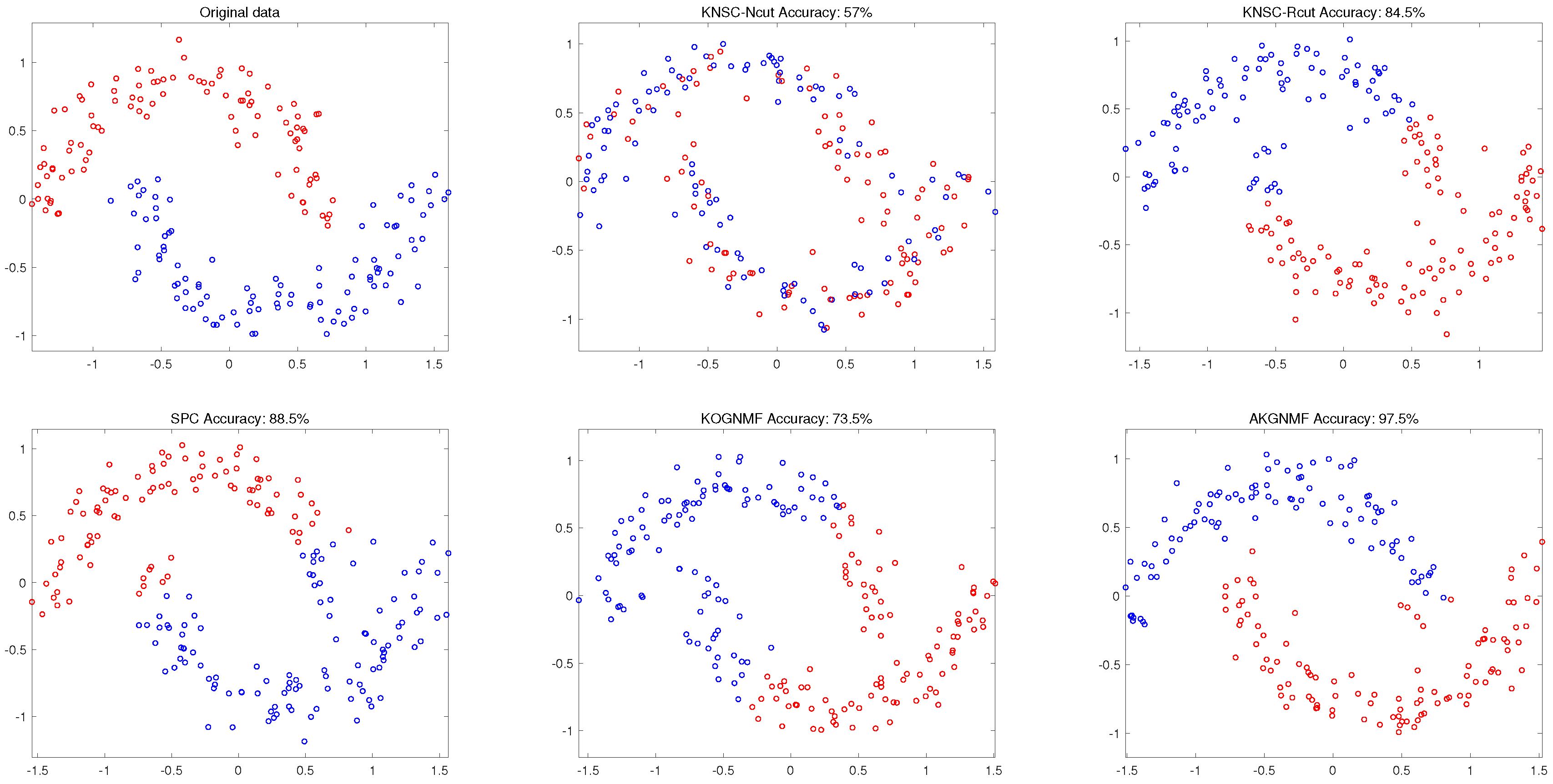
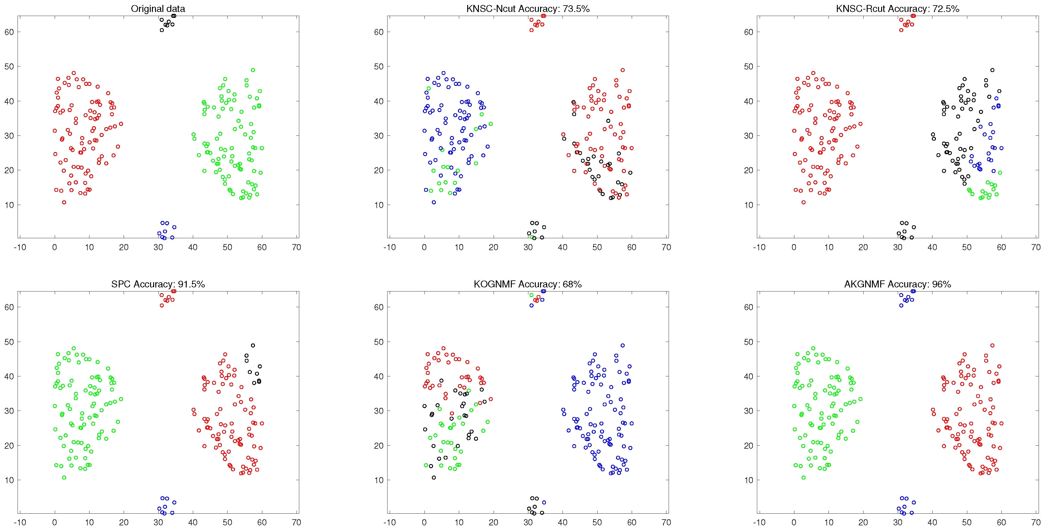
4.3.1. Clustering Results on Synthetic Data

To verify the performance of our method more intuitively, we visualize the clustering results of two synthetic datasets in Figure 1 and Figure 2. The test dataset in Figure 1 was generated with 200 points, which are distributed in the pattern of two moons. Points belonging to each moon formed a cluster. In Figure 2, a 4-cluster dataset with 200 points is produced. From Figure 1 and Figure 2, AKGNMF can process the data well with nonlinearity. Significantly, AKGNMF separates the nonlinear clusters with higher clustering accuracy compared with other methods.

4.3.2. Clustering Results on Real Data

For each of the compared methods, we followed the recommended parameter range in the original paper and used the optimal parameter group. We present the best performance and the mean value after 20 independent runs.

Figure 3 compares the accuracy results of kernel-based clustering methods on all datasets. AKGNMF can achieve the best accuracy in most datasets, showing its advantages in capturing nonlinear manifold structures.

Table 4. Clustering results measured on benchmark datasets.

Datasets	Kmeans	NMF	GNMF	CAN	KNSC-RCut	KNSC-NCut	KOGNMF	SPC	AKGNMF
(a) Accuracy (%)
Soybean	72.34	72.34	89.36	74.46	100 (73.82)	85.10 (72.02)	100 (75.10)	97.87 (76.59)	100 (79.78)
Dermatology	94.26	72.95	81.97	95.36	95.90 (84.04)	93.44 (77.19)	95.90 (85.64)	80.60 (78.94)	97.54 (90.56)
Glass	54.21	22.42	46.72	51.40	52.80 (43.06)	48.59 (46.98)	55.14 (43.01)	52.33 (45.46)	62.14 (47.78)
Vehicle	45.27	38.41	45.03	40.54	45.86 (45.48)	43.97 (41.01)	46.09 (45.75)	40.30 (39.00)	51.77 (47.28)
YALE	38.18	42.42	50.30	42.42	61.21 (51.69)	52.12 (45.66)	58.18 (52.18)	60.60 (53.12)	64.24 (55.87)
JAFFE	84.04	82.62	96.71	96.71	96.24 (84.27)	93.42 (74.24)	96.71 (84.88)	97.65 (87.53)	97.18 (87.46)
TDT2	50.38	41.19	57.73	14.24	80.55 (66.09)	50.38 (48.95)	75.65 (66.97)	71.97 (70.82)	86.67 (71.15)
(b) NMI (%)
Soybean	71.08	71.56	81.49	71.38	100 (71.30)	76.02 (67.72)	100 (72.90)	73.67 (73.63)	100 (77.28)
Dermatology	89.47	82.30	85.31	91.18	91.79 (86.80)	87.96 (84.51)	92.33 (86.38)	74.40 (71.41)	92.59 (86.00)
Glass	36.41	2.88	35.53	30.85	32.33 (27.87)	27.76 (23.88)	32.77 (29.15)	33.07 (20.75)	31.75 (22.41)
Vehicle	18.14	10.60	17.25	15.52	18.86 (18.55)	19.47 (15.36)	19.71 (19.22)	12.87 (12.57)	20.91 (18.42)
YALE	45.07	48.41	53.01	45.60	62.12 (55.21)	54.16 (50.04)	61.38 (55.65)	58.62 (54.99)	63.56 (58.89)
JAFFE	88.13	85.03	96.23	96.23	95.52 (87.74)	91.77 (79.53)	96.23 (87.94)	96.43 (91.81)	96.23 (89.96)
TDT2	44.98	35.48	51.80	3.62	71.66 (60.75)	46.66 (41.04)	69.58 (61.00)	74.16 (68.48)	67.71 (61.30)
(c) Purity (%)
Soybean	78.72	78.72	89.36	78.72	100  (79.46)	85.10 (76.38)	100 (79.78)	97.87 (76.59)	100 (83.72)
Dermatology	94.26	84.70	85.79	95.36	95.90 (91.07)	93.44 (85.90)	95.90 (91.17)	81.14 (79.53)	97.54 (91.33)
Glass	58.41	38.78	53.27	54.20	60.74 (58.20)	49.53 (47.71)	61.21 (58.92)	57.00 (46.23)	65.31 (49.15)
Vehicle	45.27	38.77	45.03	41.25	45.86 (45.48)	46.80 (41.57)	46.09 (45.75)	40.30 (39.23)	51.77 (47.28)
YALE	40.00	44.24	52.12	44.24	61.81 (52.69)	53.93 (47.66)	58.78 (53.18)	61.21 (54.63)	64.84 (57.33)
JAFFE	85.91	84.97	96.71	96.71	96.24 (86.94)	93.42 (77.34)	96.71 (86.90)	97.65 (89.57)	97.18 (89.38)
TDT2	52.67	43.95	58.80	14.85	80.55 (67.31)	50.38 (50.17)	75.80 (68.13)	74.42 (72.62)	86.67 (72.37)

The best results for every dataset are highlighted in boldface, and the average performances are shown in parentheses.

records results of all methods on all datasets using the evaluation metrics of accuracy, NMI, and purity. The best results for every dataset are highlighted in boldface, and the average performances are shown in parentheses. AKGNMF outperformed other methods in most cases, as follows.

(1)

In all the experiments except that with the JAFFE dataset, AKGNMF performed better than the other NMF-based and graph-based clustering approaches. For the JAFFE dataset, AKGNMF also presented competitive clustering accuracy.

(2)

For NMF and GNMF, the accuracy of AKGNMF on the Glass dataset increased by 39.72% and 15.42%, respectively. Accuracy also improves by 45.48% and 28.94% for the TDT2 dataset. Hence, this demonstrates the ability of graph learning to adaptively capture structural information.

(3)

With respect to k-means and the recently proposed kernel-based non-negative spectral clustering methods KNSC-Ncut and KNSC-Rcut, the improvement is promising. When comparing these three methods, the accuracy of AKGNMF for all datasets was found to be the highest.

(4)

Instead of directly constructing linear graph adjacency matrix in KOGNMF, AKGNMF obtains the optimal similarity matrix in the same nonlinear feature space as matrix factorization. A better graph structure boosts the data-representation performance of KNMF, which leads to better clustering performance of the AKGNMF method. For example, compared with KOGNMF, in TDT2, Glass and YALE datasets, the best accuracy of AKGNMF was found to improved by 11.02%, 7% and 6.06%, respectively.

(5)

In terms of similarity preservation, CAN mainly focuses on local similarity, which may ignore global similarity and lead to suboptimal results. The global structural information obtained using the AKGNMF method from high-dimensional maps is more advantageous on most datasets. Compared with SPC, we learned the nonlinear graph structure combined with the inherent potential features of NMF, and considered both the kernelized input data and the factorized representation, thereby realizing better performance of the proposed method in clustering tasks. As the results show, the best performance of AKGNMF in the dermatology dataset was improved by 16.94%, 18.19%, and 16.40% in terms of accuracy, NMI, and purity metrics, respectively; and the average performance was improved by 11.62%, 14.59%, and 11.8%, respectively.

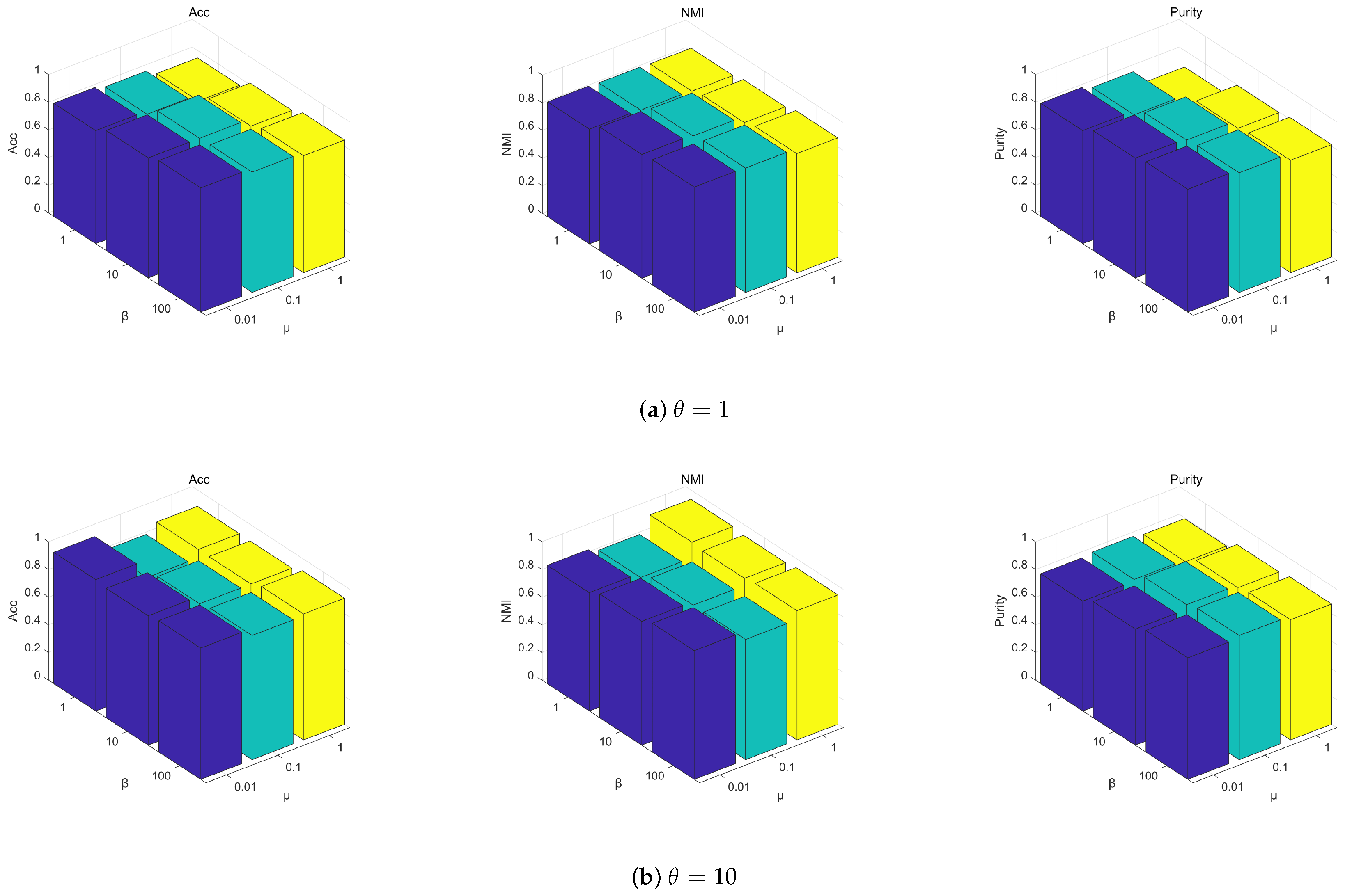
4.4. Parameter Analysis

The AKGNMF algorithm’s multiplicative rules involve the following five parameters: $\beta$, $\gamma$, $\mu$, $\theta$ and a Gaussian kernel with $\sigma$. In the adopted method, we used the Gaussian kernel and defined it as $\mathbf{K}(X_i,X_j)=exp(-\parallel x_i-x_j{\parallel }^2/{\sigma }^2)$, where $\sigma$ is the kernel width. To choose an appropriate value of the parameter $\sigma$, a grid search was performed for 40 values of $\sigma$ in the range of [0.1, 4] with a step size of $\Delta \sigma$ = 0.1 for datasets Dermatology, Glass, Soybean, JAFFE and YALE. For the Vehicle and TDT2 datasets, the process is in the range $\sigma$ = [10, 100] with $\Delta \sigma$ = 10 (step size). For the trade-off parameter $\gamma$, we also used the grid search in the range of [0.001, 100] in the same way. The important parameters mainly analyzed and discussed are $\theta$, $\beta$ and $\mu$. As mentioned previously, $\theta$ represents the similarity-preserving capability, $\beta$ corresponds to the graph regularization and $\mu$ is a trade-off parameter for the regularization term of $\mathbf{S}$. Take the JAFFE dataset as an example, which demonstrates the sensitivity of our model to the parameters shown in Figure 4, which works well over a relatively wide range of values.

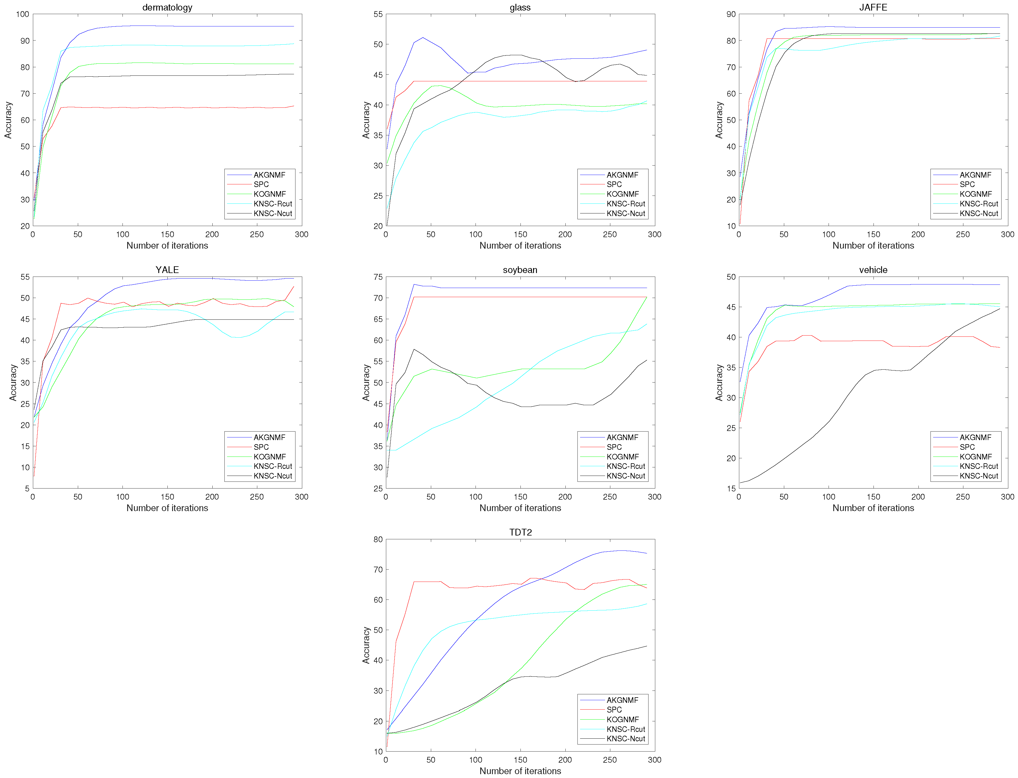
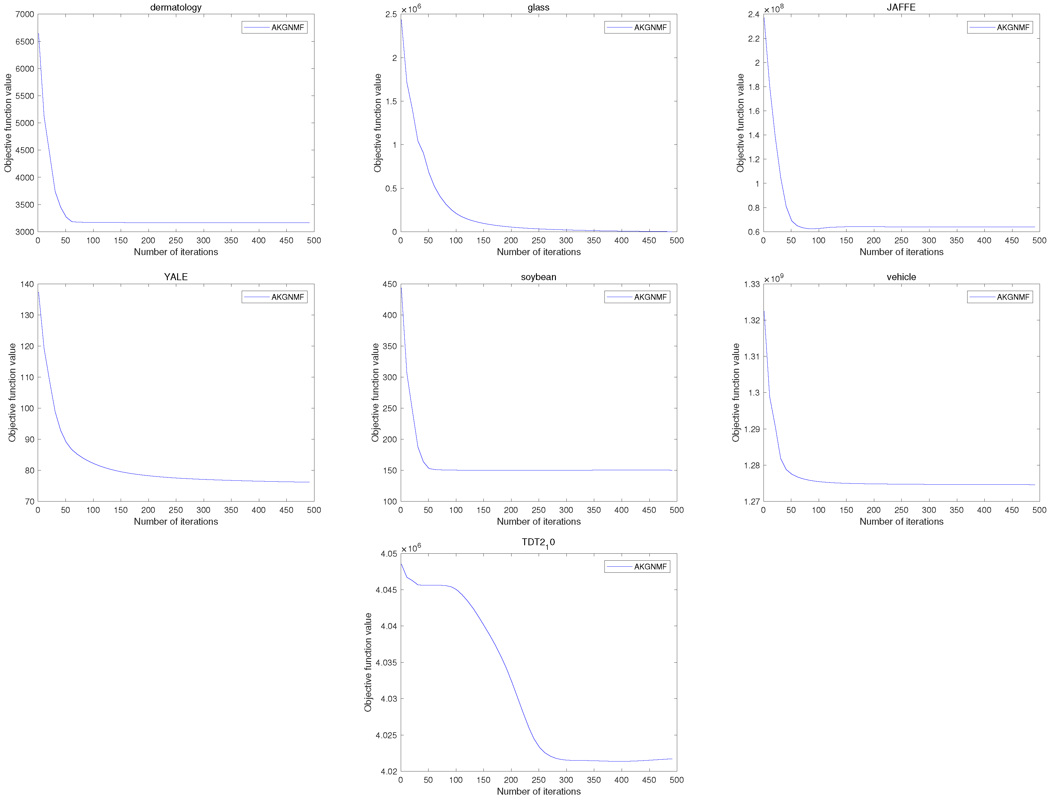
4.5. Convergence Study

The proposed updating rules for minimizing the objective function of AKGNMF are essentially iterative. We performed a theoretical analysis to prove the convergence of the proposed optimization algorithm. In this subsection, we investigate some examples to further empirically prove this.

Figure 5 shows the convergence curves of AKGNMF on all datasets. For each figure, the y-axis is the value of the objective function, and the x-axis denotes the iteration number. It can be observed that the objective function indeed decreases its value and the objective value sequences tend to converge within about 100 iterations on most datasets, which verifies the convergence and effectiveness of the proposed AKGNMF method.

5. Conclusions

In this paper, we proposed a novel kernel graph regularized nonlinear nonnegative matrix-factorization method, termed adaptive kernel graph nonnegative matrix factorization (AKGNMF). We formulated a novel framework to jointly learn an optimal graph similarity matrix and perform nonnegative matrix factorization in the kernel space. The learning process could effectively help to discover the nonlinear characteristics of input data. Moreover, an efficient iterative algorithm to solve the problem was developed. Extensive experiments were conducted on seven benchmark datasets, and the results demonstrate the superior performance of AKGNMF compared with the state-of-the-art methods.

There are many research issues worthy of exploration in future work. For example, considering the high computational complexity of graph-learning operations, it is worth trying to further enhance the efficiency. In addition, we will consider combining graph-learning-based NMF with deep neural networks for improved performance in the nonlinear representation of data.

References

1. Li, X.; Cui, G.; Dong, Y. Graph Regularized Non-Negative Low-Rank Matrix Factorization for Image Clustering. IEEE Trans. Cybern. 2016, 47, 3840–3853. [Google Scholar] [CrossRef] [PubMed]
2. Ye, R.; Li, X. Compact Structure Hashing via Sparse and Similarity Preserving Embedding. IEEE Trans. Cybern. 2015, 46, 718–729. [Google Scholar] [CrossRef]
3. Fang, X.; Xu, Y.; Li, X.; Fan, Z.; Liu, H.; Chen, Y. Locality and Similarity Preserving Embedding for Feature Selection. Neurocomputing 2014, 128, 304–315. [Google Scholar] [CrossRef]
4. Yang, Y.; Shen, H.; Nie, F.; Ji, R.; Zhou, X. Nonnegative Spectral Clustering with Discriminative Regularization. In Proceedings of the AAAI Conference on Artificial Intelligence, San Francisco, CA, USA, 7–11 August 2011; Volume 25, pp. 555–560. [Google Scholar]
5. Peng, C.; Kang, Z.; Cai, S.; Cheng, Q. Integrate and Conquer: Double-Sided Two-Dimensional k-Means via Integrating of Projection and Manifold Construction. ACM Trans. Intell. Syst. Technol. (TIST) 2018, 9, 1–25. [Google Scholar] [CrossRef]
6. Elkan, C. Using the Triangle Inequality to Accelerate k-Means. In Proceedings of the 20th International Conference on Machine Learning (ICML-03), Washington, DC, USA, 21–24 August 2003; pp. 147–153. [Google Scholar]
7. Hou, C.; Nie, F.; Yi, D.; Tao, D. Discriminative Embedded Clustering: A Framework for Grouping High-Dimensional Data. IEEE Trans. Neural Netw. Learn. Syst. 2014, 26, 1287–1299. [Google Scholar] [PubMed]
8. Kang, Z.; Xu, H.; Wang, B.; Zhu, H.; Xu, Z. Clustering With Similarity Preserving. Neurocomputing 2019, 365, 211–218. [Google Scholar] [CrossRef] [Green Version]
9. Kang, Z.; Lu, Y.; Su, Y.; Li, C.; Xu, Z. Similarity Learning via Kernel Preserving Embedding. In Proceedings of the AAAI Conference on Artificial Intelligence, Honolulu, HI, USA, 27 January–1 February 2019; Volume 33, pp. 4057–4064. [Google Scholar]
10. Zeng, K.; Yu, J.; Li, C.; You, J.; Jin, T. Image Clustering by Hyper-Graph Regularized Non-Negative Matrix Factorization. Neurocomputing 2014, 138, 209–217. [Google Scholar] [CrossRef]
11. Lu, Y.; Lai, Z.; Xu, Y.; You, J.; Li, X.; Yuan, C. Projective Robust Nonnegative Factorization. Inf. Sci. 2016, 364, 16–32. [Google Scholar] [CrossRef]
12. Maisog, J.M.; DeMarco, A.T.; Devarajan, K.; Young, S.; Fogel, P.; Luta, G. Assessing Methods for Evaluating the Number of Components in Non-Negative Matrix Factorization. Mathematics 2021, 9, 2840. [Google Scholar] [CrossRef]
13. Turk, M.; Pentland, A. Eigenfaces for Recognition. J. Cogn. Neurosci. 1991, 3, 71–86. [Google Scholar] [CrossRef]
14. Hyvärinen, A.; Oja, E. Independent Component Analysis: Algorithms and Applications. Neural Netw. 2000, 13, 411–430. [Google Scholar] [CrossRef] [PubMed] [Green Version]
15. Dunteman, G.H. Principal Components Analysis; Sage: Newbury Park, CA, USA, 1989; Number 69. [Google Scholar]
16. Liu, W.; Zheng, N. Non-Negative Matrix Factorization Based Methods for Object Recognition. Pattern Recognit. Lett. 2004, 25, 893–897. [Google Scholar] [CrossRef]
17. Févotte, C.; Idier, J. Algorithms for Nonnegative Matrix Factorization with the β-Divergence. Neural Comput. 2011, 23, 2421–2456. [Google Scholar] [CrossRef]
18. Belkin, M.; Niyogi, P.; Sindhwani, V. Manifold Regularization: A Geometric Framework for Learning From Labeled and Unlabeled Examples. J. Mach. Learn. Res. 2006, 7, 2399–2434. [Google Scholar]
19. Xu, Z.; King, I.; Lyu, M.R.T.; Jin, R. Discriminative Semi-supervised Feature Selection via Manifold Regularization. IEEE Trans. Neural Networks 2010, 21, 1033–1047. [Google Scholar] [PubMed]
20. Huang, S.; Xu, Z.; Wang, F. Nonnegative Matrix Factorization With Adaptive Neighbors. In Proceedings of the 2017 International Joint Conference on Neural Networks (IJCNN), Anchorage, AK, USA, 14–19 May 2017; pp. 486–493. [Google Scholar]
21. Lee, D.D.; Seung, H.S. Learning the Parts of Objects by Non-Negative Matrix Factorization. Nature 1999, 401, 788–791. [Google Scholar] [CrossRef]
22. Cai, D.; He, X.; Han, J.; Huang, T.S. Graph Regularized Nonnegative Matrix Factorization for Data Representation. IEEE Trans. Pattern Anal. Mach. Intell. 2010, 33, 1548–1560. [Google Scholar]
23. Tolić, D.; Antulov-Fantulin, N.; Kopriva, I. A Nonlinear Orthogonal Non-Negative Matrix Factorization Approach to Subspace Clustering. Pattern Recognit. 2018, 82, 40–55. [Google Scholar] [CrossRef] [Green Version]
24. Huang, J.; Nie, F.; Huang, H. A New Simplex Sparse Learning Model to Measure Data Similarity for Clustering. In Proceedings of the Twenty-Fourth International Joint Conference on Artificial Intelligence, Buenos Aires, Argentina, 25–31 July 2015. [Google Scholar]
25. Kang, Z.; Peng, C.; Cheng, Q.; Xu, Z. Unified Spectral Clustering With Optimal Graph. In Proceedings of the AAAI Conference on Artificial Intelligence, New Orleans, LA, USA, 2–7 February 2018; Volume 32. [Google Scholar]
26. Ge, H.; Song, A. A New Low-Rank Structurally Incoherent Algorithm for Robust Image Feature Extraction. Mathematics 2022, 10, 3648. [Google Scholar] [CrossRef]
27. Zhang, L.; Zhang, Q.; Du, B.; You, J.; Tao, D. Adaptive Manifold Regularized Matrix Factorization for Data Clustering. In Proceedings of the 6th International Joint Conference on Artificial Intelligence, Melbourne, Australia, 9–25 August 2017; pp. 3399–3405. [Google Scholar]
28. Peng, Y.; Long, Y.; Qin, F.; Kong, W.; Nie, F.; Cichocki, A. Flexible Non-Negative Matrix Factorization With Adaptively Learned Graph Regularization. In Proceedings of the ICASSP 2019—2019 IEEE International Conference on Acoustics, Speech and Signal Processing (ICASSP), Brighton, UK, 12–17 May 2019; pp. 3107–3111. [Google Scholar] [CrossRef]
29. Huang, S.; Xu, Z.; Kang, Z.; Ren, Y. Regularized Nonnegative Matrix Factorization With Adaptive Local Structure Learning. Neurocomputing 2020, 382, 196–209. [Google Scholar] [CrossRef]
30. Yi, Y.; Wang, J.; Zhou, W.; Zheng, C.; Kong, J.; Qiao, S. Non-negative Matrix Factorization With Locality Constrained Adaptive Graph. IEEE Trans. Circuits Syst. Video Technol. 2019, 30, 427–441. [Google Scholar] [CrossRef]
31. Chen, K.; Che, H.; Li, X.; Leung, M.F. Graph Non-Negative Matrix Factorization with Alternative Smoothed L0 Regularizations. Neural Comput. Appl. 2022, 1–15. [Google Scholar]
32. Yang, X.; Che, H.; Leung, M.F.; Liu, C. Adaptive Graph Nonnegative Matrix Factorization With the Self-Paced Regularization. Appl. Intell. 2022, 1–18. [Google Scholar] [CrossRef]
33. Paatero, P.; Tapper, U. Positive Matrix Factorization: A Non-Negative Factor Model With Optimal Utilization of Error Estimates of Data Values. Environmetrics 1994, 5, 111–126. [Google Scholar] [CrossRef]
34. Nie, F.; Wang, X.; Huang, H. Clustering and Projected Clustering with Adaptive Neighbors. In Proceedings of the 20th ACM SIGKDD International Conference on Knowledge Discovery and Data Mining, New York, NY, USA, 24–27 August 2014; KDD ’14. pp. 977–986. [Google Scholar] [CrossRef]
35. Zhu, X.; Zhang, S.; Hu, R.; Zhu, Y.; Song, J. Local and Global Structure Preservation for Robust Unsupervised Spectral Feature Selection. IEEE Trans. Knowl. Data Eng. 2017, 30, 517–529. [Google Scholar] [CrossRef]
36. Ren, Z.; Sun, Q. Simultaneous Global and Local Graph Structure Preserving for Multiple Kernel Clustering. IEEE Trans. Neural Networks Learn. Syst. 2020, 32, 1839–1851. [Google Scholar] [CrossRef]
37. Ding, C.H.; Li, T.; Jordan, M.I. Convex and Semi-Nonnegative Matrix Factorizations. IEEE Trans. Pattern Anal. Mach. Intell. 2008, 32, 45–55. [Google Scholar] [CrossRef] [Green Version]
38. White, S.; Smyth, P. A Spectral Clustering Approach to Finding Communities in Graphs. In Proceedings of the 2005 SIAM International Conference on Data Mining, Newport Beach, CA, USA, 21–23 April 2005; pp. 274–285. [Google Scholar]
39. He, X.; Niyogi, P. Locality Preserving Projections. Adv. Neural Inf. Process. Syst. 2004, 16, 153–160. [Google Scholar]
40. Belkin, M.; Niyogi, P. Laplacian Eigenmaps for Dimensionality Reduction and Data Representation. Neural Comput. 2003, 15, 1373–1396. [Google Scholar] [CrossRef] [Green Version]
41. Cai, D.; Wang, X.; He, X. Probabilistic Dyadic Data Analysis With Local and Global Consistency. In Proceedings of the 26th Annual International Conference on Machine Learning, Montreal, QC, Canada, 14–18 June 2009; pp. 105–112. [Google Scholar]
42. Huang, T.M.; Kecman, V.; Kopriva, I. Kernel Based Algorithms for Mining Huge Data Sets; Springer: Warsaw, Poland, 2006; Volume 1. [Google Scholar]
43. Boyd, S.; Boyd, S.P.; Vandenberghe, L. Convex Optimization; Cambridge University Press: Cambridge, UK, 2004. [Google Scholar]
44. Michalski, R.S. Learning by Being Told and Learning by Examples: An Experimental Comparison of the Two Methods of Knowledge Acquisition in the Context of Developing an Expert System for Soybean Disease Analysis. Int. J. Policy Anal. Inf. Syst. 1980, 4, 125–161. [Google Scholar]
45. Güvenir, H.A.; Demiröz, G.; Ilter, N. Learning Differential Diagnosis of Erythemato-Squamous Diseases Using Voting Feature Intervals. Artif. Intell. Med. 1998, 13, 147–165. [Google Scholar] [CrossRef] [Green Version]
46. Evett, I.W.; Spiehler, E.J. Rule Induction in Forensic Science; Halsted Press: Pinner, UK, 1989; pp. 152–160. [Google Scholar]
47. Siebert, J.P. Vehicle Recognition Using Rule Based Methods; Turing Institute: Glasgow, Scotland, 1987. [Google Scholar]
48. Cai, D.; He, X.; Han, J. Locally Consistent Concept Factorization for Document Clustering. IEEE Trans. Knowl. Data Eng. 2010, 23, 902–913. [Google Scholar] [CrossRef] [Green Version]
49. Georghiades, A.S.; Belhumeur, P.N.; Kriegman, D.J. From Few to Many: Illumination Cone Models for Face Recognition Under Variable Lighting and Pose. IEEE Trans. Pattern Anal. Mach. Intell. 2001, 23, 643–660. [Google Scholar] [CrossRef] [Green Version]
50. Lyons, M.J.; Kamachi, M.; Gyoba, J. Coding Facial Expressions With Gabor Wavelets (IVC Special Issue). arXiv 2020, arXiv:2009.05938. [Google Scholar]
51. MacQueen, J. Some Methods for Classification and Analysis of Multivariate Observations. In Proceedings of the Fifth Berkeley Symposium on Mathematical Statistics and Probability, Oakland, CA, USA; University of California Press: Berkeley, CA, USA, 1967; Volume 1, pp. 281–297. [Google Scholar]
52. Lee, D.; Seung, H.S. Algorithms for Non-negative Matrix Factorization. In Proceedings of the 14th Annual Neural Information Processing Systems Conference, Denver, CO, USA, 27 November–2 December 2000; pp. 556–562. [Google Scholar]
53. Hoyer, P.O. Non-Negative Sparse Coding. In Proceedings of the 12th IEEE Workshop on Neural Networks for Signal Processing, Martigny, Switzerland, 4–6 September 2002; pp. 557–565. [Google Scholar]
Figure 1. The two-moon dataset clustering results.
Information 14 00208 g001
Figure 2. The 4-cluster dataset clustering results.
Information 14 00208 g002
Figure 3. The clustering accuracy of kernel methods for the independent number of iterations on 7 datasets.
Information 14 00208 g003
Figure 4. The influences of parameters on the JAFFE dataset.
Information 14 00208 g004
Figure 5. Convergence curve of AKGNMF.
Information 14 00208 g005