Article

A Thorough Reproducibility Study on Sentiment Classification: Methodology, Experimental Setting, Results

by
Giorgio Maria Di Nunzio
1,*,† and
Riccardo Minzoni
2,†
1
Department of Information Engineering, University of Padova, 35122 Padova, Italy
2
Department of Mathematics, University of Padova, 35122 Padova, Italy
*
Author to whom correspondence should be addressed.
These authors contributed equally to this work.
Information 2023, 14(2), 76; https://doi.org/10.3390/info14020076
Submission received: 21 December 2022 / Revised: 14 January 2023 / Accepted: 18 January 2023 / Published: 28 January 2023
(This article belongs to the Special Issue Feature Papers in Information in 2023)

Abstract

:
A survey published by Nature in 2016 revealed that more than 70% of researchers failed in their attempt to reproduce another researcher’s experiments, and over 50% failed to reproduce one of their own experiments; a state of affairs that has been termed the ‘reproducibility crisis’ in science. The purpose of this work is to contribute to the field by presenting a reproducibility study of a Natural Language Processing paper about “Language Representation Models for Fine-Grained Sentiment Classification”. A thorough analysis of the methodology, experimental setting, and experimental results are presented, leading to a discussion of the issues and the necessary steps involved in this kind of study.

1. Introduction

Due to advances in knowledge and technology, the fields of Artificial Intelligence (AI) and Machine Learning (ML) have grown in recent years, leading to a significant increase in published papers. Since then, one of the new challenges in machine learning research has been to ensure that presented and published results are sound and reliable [1]. Reproducibility, that is obtaining similar results as presented in a paper or talk, using the same code and data (when available), is a necessary step in verifying the reliability of research findings. Indeed, it must be considered as one of the cornerstones of scientific research: an inability to reproduce certain results is, with few exceptions, seen as casting doubt on their validity. Reproducibility is also an important step in promoting open and accessible research, thereby allowing the scientific community to quickly integrate new findings and convert ideas to practice. It also promotes the use of robust experimental workflows, which potentially reduce unintentional errors. Nevertheless, a 2016 survey [2] revealed that more than 70% of researchers failed in their attempt to reproduce another researcher’s experiments, and over 50% failed to reproduce one of their own experiments; a state of affairs that has been termed the ‘reproducibility crisis’ in science. After the publication of this article, the research community has started to pay more and more attention to this problem. Some examples are the following: (for this brief review of the literature, we searched on Google Scholar for the most important articles, in terms of high-impact journals in Computer Science, for each year from 2017 until 2023 about “reproducibility crisis” in “computer science”).
  • The main aim of [3] is to make a library of semantic similarity measures publicly available for the first time, together with a set of reproducible experiments whose aims are the exact replication of three experimental surveys. In addition, the authors propose a self-contained experimental platform which can be easily used for extensive experimentation, even with no software coding.
  • In [4], the authors present a number of controllable environment settings that often go unreported, and illustrate that these are factors that can cause irreproducibility of results as presented in the literature. These environmental factors have an effect on the effectiveness of neural networks due to the non-convexity of the optimization surface.
  • In the study proposed by [5], the focus is on the communication aspect, investigating students’ current understanding of reproducibility, whether they are able to communicate reproducible data analysis, and if not, what skills are missing and what types of training can be helpful. Training on reproducible data analysis should be an indispensable component in data science education.
  • The authors of [6] review the extent and causes of the replication crisis in many areas of science, with a focus on issues relating to the use of null hypothesis significance as an evidentiary criterion. They also discuss alternative ways for analyzing data and present evidence for hypothesized effects. They also argue for improved openness and transparency in experimental research.
  • In [7], the authors attempt a complete reproduction of five automatic malware detectors from the literature, and they discuss to what extent they are reproducible. In particular, they provide insights on the implications around the guesswork that may be required to finalize a working implementation.
  • A survey of machine learning platforms with the aim of studying whether they provide features that simplify making experiments reproducible out-of-the-box [8] showed that none of the studied platforms support this feature set; moreover, the experiment reveals a statistically significant difference in results when the exact same experiment is conducted on different data sets.
  • In [9], the authors propose a methodological approach that not only provides a replicable experimental analysis but also provides researchers with a workflow using existing tools that can be transposed to other domains with only little manual work.
In Table 1, we show a summary of the main findings of these papers.
The past few years have seen an impressive range of new initiatives and events in the fields of Natural Language Processing (NLP) and Information Retrieval (IR) that address how reproducibility should be defined, measured and addressed. For instance, in 2019, the Neural Information Processing Systems (NeurIPS) (https://reproducibility-challenge.github.io/neurips2019/ (accessed on 19 January 2023)) conference, the premier international conference for research in machine learning, introduced a reproducibility program, designed to improve standards across the community for how we conduct, communicate, and evaluate machine learning research. The program contained three components: a code submission policy, a community-wide reproducibility challenge, and the inclusion of the Machine Learning Reproducibility checklist as part of the paper submission process [10], later also adopted by EMNLP’20 (https://2020.emnlp.org/blog/2020-05-20-reproducibility (accessed on 19 January 2023)) and AAAI’21 (https://aaai.org/Conferences/AAAI-21/reproducibility-checklist/ (accessed on 19 January 2023)). Other conferences have foregrounded reproducibility via calls, chairs’ blogs, special themes and social media posts. Sharing code, data and supplementary material providing details about data, systems, and training regimes is firmly established in the ML/NLP/IR community, with virtually all main events now encouraging and making space for it (https://ecir2020.org/call-for-reproducibility-papers/, https://sigir.org/sigir2022/call-for-reproducibility-track-papers/ (accessed on 19 January 2023)).
The purpose of this work is to contribute to this field of research by reproducing the experiment and results from the 2020 paper “Language Representation Models for Fine-Grained Sentiment Classification” [11]. The chosen NLP task is sentiment classification, where the aim is detecting positive or negative sentiments in text [12]. The discussion will be centered on the methodology employed during the experiment, and the techniques used to replicate the results and the evaluation methods applied by the authors. The project is mainly focused on the BERT architecture (Bidirectional Encoder Representation from Transformers) created by Google AI [13], which is a neural network that relies entirely on attention mechanism, and its alternatives, by means of several approaches.
We will discuss the (few) flaws and inconsistencies of the original paper and comment on the source code step by step. We will reason about the mistakes, what derived from such errors, and suggest a method for recovering from that, after trying to reproduce the stated results with the available tools. We also provide the source code of our paper (https://github.com/riccardominzoni/reproducibilitycasestudy (accessed on 19 January 2023)).
The paper is organized as follows: First of all, in Section 2, we define the terminology used to define what reproducibility means at the international level; in Section 3, we introduce the original article and present the task, the dataset, and the methodology used. Section 4 describes the setting of the experiment in detail to reproduce the original paper, while in Section 5, the results of the reproducibility experiment are discussed. We give our final remarks in Section 7.

2. Terminology for Reproducing Experiments

Before going any further, it is worth defining a few terms that have been used (sometimes interchangeably) to describe reproducibility and related concepts. Reproducibility research uses a wide range of closely related terms, often with conflicting meanings, including reproducibility, repeatability, replicability, recreation, re-run, robustness, repetition, and generalizability. The two most frequently used ‘R-terms’, reproducibility and replicability, are also the most problematic, with several different definitions. For instance, the ACM (Association for Computing Machinery, 2020) (https://www.acm.org/publications/policies/artifact-review-badging (accessed on 19 January 2023)), has stated that results have been reproduced if “obtained in a subsequent study by a person or team other than the authors, using, in part, artifacts provided by the author”, and replicated if “obtained in a subsequent study by a person or team other than the authors, without the use of author-supplied artifacts”. The definitions are tied to team and software (artifacts), but it is unclear how much of the latter have to be the same for reproducibility, and how different the team needs to be for either concept. Instead, “Reproducing the result of a computation means running the same software on the same input data and obtaining the same results. […] Replicating a published result means writing and then running new software based on the description of a computational model or method provided in the original publication, and obtaining results that are similar enough to be considered equivalent”. are the definitions tied to new vs. original software given by Rougier et al. [14]. It is clear from the many reports of failures to obtain the ‘same results’ with the ‘same software and data’ in recent years that the above definitions raise practical questions, such as how to tell the ‘same software’ from ‘new software’, and how to determine the equivalence of results. Wieling et al. [15] define reproducibility as “the exact re-creation of the results reported in a publication using the same data and methods”, but then discuss (the failure of) replicating results without defining that term. In contrast, some scientists, i.e., Whitaker [16], decided to tie definitions to data as well as code; see Table 2.
The International Vocabulary of Metrology (VIM) [18] offers a common terminological denominator thanks to extreme precision of the definitions used. The VIM definitions of reproducibility and repeatability (no other R-terms are defined) are entirely general, made possible by two key differences compared to the NLP/ML definitions above. Firstly, in a key conceptual shift, reproducibility and repeatability are properties of measurements (not of systems or abstract findings). The important difference is that the concept of reproducibility now references a specified way of obtaining a measured quantity value (which can be an evaluation metric, statistical measure, human evaluation method, etc. in NLP). Secondly, reproducibility and repeatability are defined as the precision of a measurement under specified conditions, i.e., the distribution of the quantity values obtained in repeat (or replicate) measurements.
In VIM, repeatability is the precision of measurements of the same or similar object obtained under the same conditions, as captured by a specified set of repeatability conditions, whereas reproducibility is the precision of measurements of the same or similar object obtained under different conditions, as captured by a specified set of reproducibility conditions. To make the VIM terms more recognizable in an NLP context, we also call repeatability reproducibility under the same conditions, and (VIM) reproducibility reproducibility under varied conditions  [17].
Reproduction under the same conditions means the closest thing to an exact recreation or reuse of an existing system and evaluation set-up, as well as a comparison of results, while reproduction under varied conditions can be explained as a reproduction study with deliberate variation of one or more aspects of the system and/or measurement, as well as a comparison of results. Since in our experiment, there is variation of aspects of the system and variation inside the code, we will refer to our work as a reproducibility study.

3. Case Study

This reproducibility study began around the second semester of 2021. At that time, we carried out a search of the most recent papers on sentiment classification that had the following requirements: a standard benchmark, source code available in Python, and state-of-the-art results. The paper that met all these conditions was “Language Representation Models for Fine-Grained Sentiment Classification” [11], published in May 2020 by Cheang et al. The paper under examination was posted on the ‘Papers with code’ platform (https://paperswithcode.com/paper/language-representation-models-for-fine (accessed on 19 January 2023)), and the dataset also has a track record as one of the best performing models in terms of accuracy (https://paperswithcode.com/sota/sentiment-analysis-on-sst-5-fine-grained (accessed on 19 January 2023)).
As the title suggests, the scope of the work was to perform a sentiment classification using a fine-grained dataset in a Natural Language Processing task. The work was intended to be a replication and subsequent extension of the work previously described in Munikar et al. (2019) [19]. It shows how the embedding tool “Bidirectional Encoder Representations from Transforms” allows a simple model to achieve state-of-the-art accuracy in the classification task using the Stanford Sentiment Tree (SST) dataset. Munikar et al. performed binary and fine-grained sentiment classifications exploiting the recently (at the time) implemented BERT model in its first two versions, BERT BASE and BERT LARGE . Since the publication of this paper in 2019, several alternatives for the BERT architecture have been published, with the three primary ones being AlBERT [20] (Lan et al., 2019), DistilBERT [21] (Sanh et al., 2019) and RoBERTa [22] (Liu et al., 2019). The authors of our case study examined whether there is an improvement when it is applied to a novel task, namely fine-grained classification, since these models reported some improvements over BERT on the popular benchmarks GLUE, SQuAD, and RACE [23], but, none of them have had been applied to the sentiment classification task yet.
The following sections describe a detailed analysis of their work: from the sentiment classification task to the dataset and the models used to classify the data.

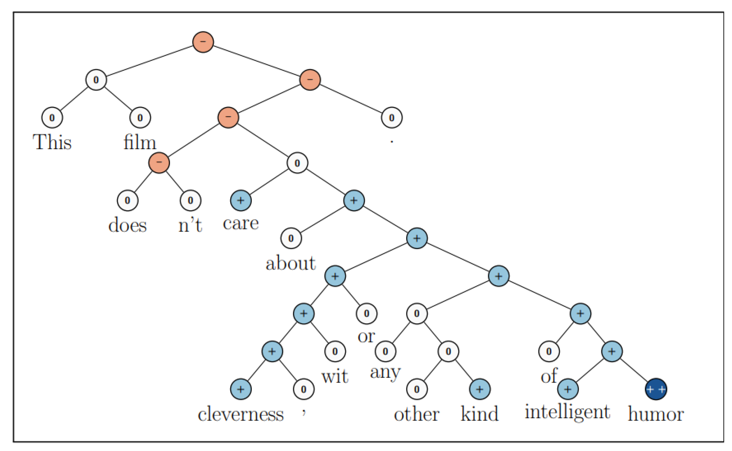
3.1. Task: Fine-Grained Sentiment Classification

The work published in the article focused on fine-grained sentiment classification and, in particular, a multi-class classification task where text can be categorized into five classes. The task is to predict whether the text (a document, a sentence, a phrase, etc.) expresses either a positive or negative sentiment.
The aim of the paper is to train a neural model (a BERT model) to classify movie reviews into five classes (negative, somewhat negative, neutral, somewhat positive, positive) based on the phrase context.

3.2. Dataset: Stanford Sentiment Tree (SST)
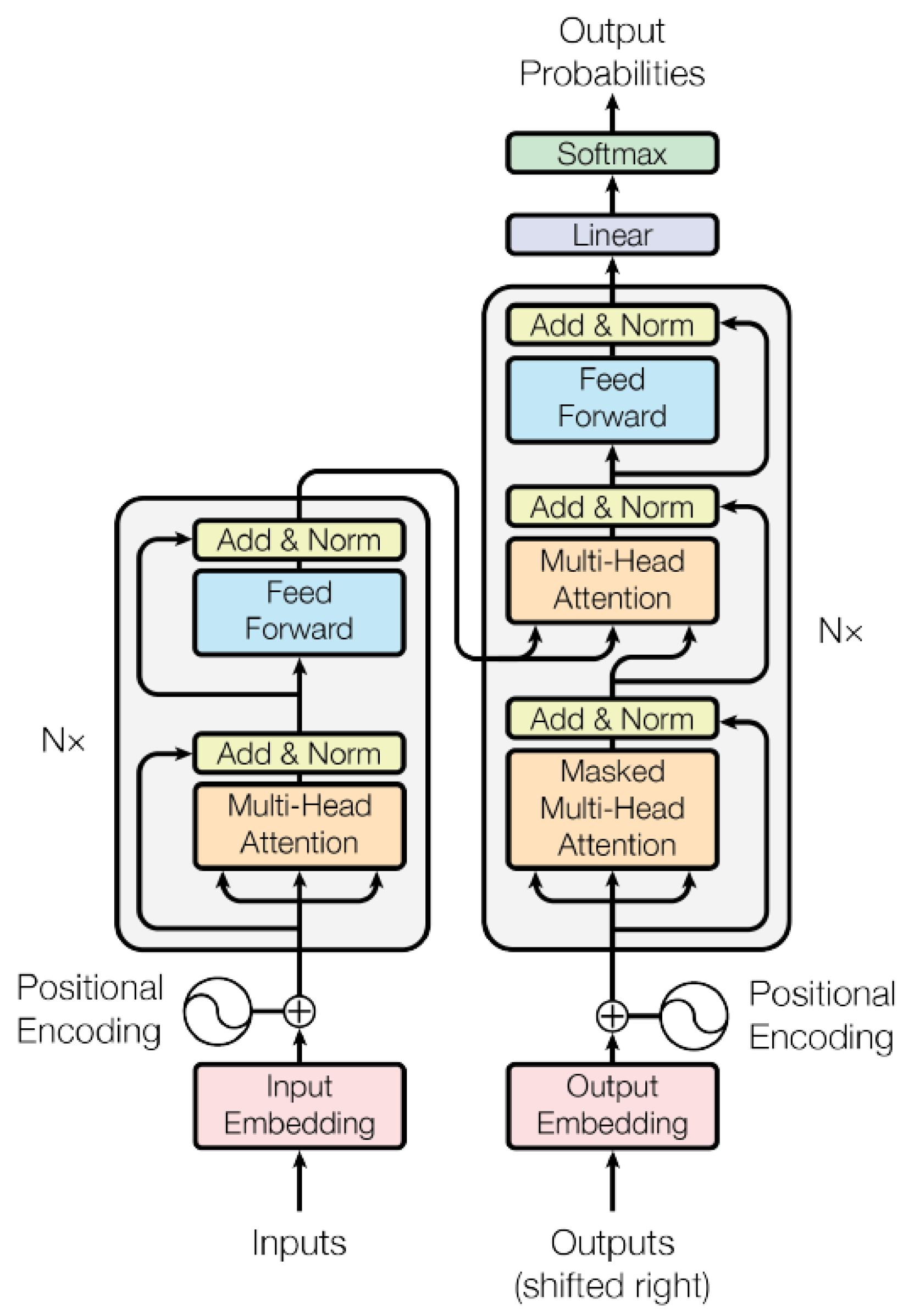
In 2013 Socher et al. [24] introduced the Stanford Sentiment Tree (SST) dataset, a collection of phrases and sentences that would become one of the most used due to its particular structure. It is the first corpus with fully labeled parse trees, which allows for a complete analysis of the compositional effects of sentiment in language.
It is based on the dataset introduced by Pang and Lee (2005) [25]. It includes 11,855 sentences extracted from movie reviews and subsequently parsed with the Stanford parser (Klein and Manning, 2003) [26], resulting in a total of 215,154 unique texts of varying lengths from those parse trees. At least three human judges labeled each word, displayed individually or in 10-g, 20-g, and full sentences on a scale from 1 to 25 (respectively very negative to very positive), paying extreme attention to not interfering with labeling and being as objective as possible.
Figure 1 shows an example with a clear compositional tree structure, with the whole sentence as the root node and the individual words as leaf nodes, and a unique label for every word, branch, and node (−−, −, 0, +, ++). We can see how the right branch is mainly labeled as positive but how, in reality, at the root level the sentence assumes a negative meaning. This is the actual meaning of compositional structure: based on the branch we are considering, the meaning of a sentence could be negative or positive, but once we encounter a negation term, the complete sentiment changes. Hence, the unique tree architecture can capture the effects of composition on sentence semantics.
The name SST-5 is used when the range from 1 to 25 is binned into five classes: very negative, negative, neutral, positive, and very positive. In Table 3, we show a breakdown of the number of labels in the dataset.

3.3. Transformers

Neural models such as transformers [27] are able to dispense with recurrence and convolutions entirely because they rely solely on attention mechanisms to draw global dependencies between input and output. The models exploited in the article are based entirely on these two concepts: attention mechanism and Transformers, and on transfer learning, a process in which a model is pre-trained and then fine-tuned for a downstream task. In recent years, thanks to their unique and innovative composition, these advanced the state-of-the-art in many popular NLP tasks, confirming the fact that transfer learning has officially become the de facto standard in almost every field of data science. Indeed, the possibility of exploiting algorithms and models which would require an enormous computational capability to be trained, but instead are already trained on general purposes, meaning that almost every computer could fine-tune them with just a few hours of training, is revolutionary. Additionally, nowadays the most famous models can be easily downloaded from their official sites, so that everyone can use them for any specific task. Our discussion continues in more detail for each model and its architecture in the following subsections.

3.3.1. BERT

At Google AI in 2019, Devlin et al. [13] created Bidirectional Encoder Representation from Transformers, BERT, a conceptually simple but, at the same time, empirically powerful architecture able to obtain new state-of-the-art results on eleven natural language processing tasks over the years. BERT is designed to pre-train deep bidirectional representations from unlabeled text by jointly conditioning on both the left and right context in all layers. This distinctive feature allows the pre-trained model to be globally prepared for any NLP task. Indeed, it can be fine-tuned with just one additional output layer at the end of the architecture in order to perform a wide range of tasks with a minimal difference between the pre-trained structure and the final downstream one. BERT’s model architecture is a multi-layer bidirectional Transformer encoder based on the original implementation described in Vaswani et al. (2017) [28].
It follows an overall encoder–decoder structure: the encoder maps an input sequence of symbol representations ( x 1 , , x n ) to a sequence of continuous representations z = ( z 1 , , z n ) . Given z, the decoder generates an output sequence ( y 1 , , y m ) of symbols one element at the time. At each step, the model is autoregressive, consuming the previously generated symbols as additional input when generating the next. In the left and right halves of Figure 2 the encoder and decoder, respectively, are shown. They both exploit stacked self-attention and pointwise, fully connected layers, giving the usual symmetrical structure but, in addition, a third layer is present in the decoder which performs a further attention mechanism. The details of the design are described as follows:
  • Encoder:
    Composed of a stack of N = 6 identical layers, each one with the two sub-layers of a multi-head self-attention mechanism and a position-wise fully connected feedforward network. A residual connection around the sub-layers, followed by layer normalization, is implemented, that is, the output of each sub-layer is L a y e r N o r m ( x + S u b l a y e r ( x ) ) , where S u b l a y e r ( x ) is the function implemented by the sub-layer itself. Outputs of the fixed dimension d m o d e l = 512 are produced by all sub-layers and the embedding layers in order to facilitate these residual connections.
  • Decoder:
    Composed of a stack of N = 6 identical layers, as well as the encoder. In addition to the two sub-layers, the decoder inserts a third sub-layer, which performs multi-head attention over the output of the encoder stack. Similar to the encoder, they employ residual connections around each of the sub-layers, followed by layer normalization. The self-attention sub-layer in the decoder stack is modified in order to prevent positions from attending to subsequent positions. This masking, combined with the fact that the output embeddings are offset by one position, ensures that the predictions for position i can depend only on the known outputs at positions less than i.

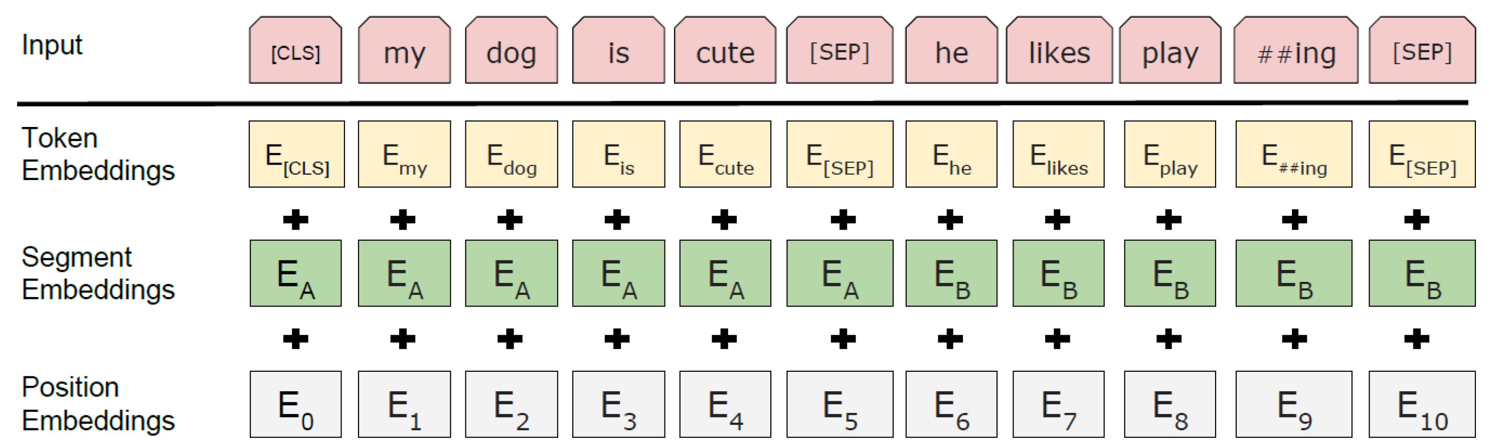
3.3.2. Word Embeddings

Since BERT can handle a variety of downstream tasks, the input representation is able to unambiguously represent both a single sentence and a pair of sentences (e.g., 〈Question, Answer〉) in one token sequence. A “sequence” refers to the input token sequence to BERT, which may be a single sentence or two sentences packed together. In order to define an input and output representation, at first WordPiece embeddings [30], with a 30,000 token vocabulary, is exploited. Next, two custom embeddings are implemented. The first token of every sequence is always a special classification token ([CLS]). The final hidden state corresponding to this token is used as the aggregate sequence representation for classification tasks. Furthermore, sentence pairs are packed together into a single sequence. They differentiate the sentences in two ways. First, they separate them with a special token ([SEP]). Second, they add a learned embedding to every token indicating whether it belongs to sentence A or sentence B. For a given token, its final input representation is constructed by summing the corresponding token, segment, and position embeddings. A visualization of this construction can be seen in Figure 3.

3.3.3. Pre-Training and Fine-Tuning

There are two existing strategies for applying pre-trained language representations to downstream tasks: f e a t u r e - b a s e d and f i n e - t u n i n g  [32]. The feature-based approach uses task-specific architectures that include the pre-trained representations as additional features. The fine-tuning approach introduces minimal task-specific parameters, and is trained on the downstream tasks by simply fine-tuning all pre-trained parameters. The two approaches share the same objective function during pre-training, where they use unidirectional language models to learn general language representations. There have been discussions about the fact that current techniques restrict the power of the pre-trained representations, especially for the fine-tuning approaches. The major limitation is that standard language models are unidirectional, and this limits the choice of architectures that can be used during pre-training. Such restrictions are suboptimal for sentence-level tasks, and could be very harmful when applying fine-tuning based approaches to token-level tasks, for example, question-answering tasks, where it is crucial to incorporate context from both directions. For this reason, BERT’s creators did not use traditional approaches but instead, they decided to pre-train the model using two unsupervised tasks:
  • Masked LM:
    Standard conditional language models can only be trained left-to-right or right-to-left, since bidirectional conditioning would allow each word to indirectly “see itself”, and the model could trivially predict the target word in a multilayered context. In order to train a deep bidirectional representation, the authors simply mask some percentage of the input tokens at random, and then predict those masked tokens.
    In all of the experiments, they mask 15 % of all WordPiece tokens in each sequence at random, and they only predict the masked words rather than reconstructing the entire input. Although this allows them to obtain a bidirectional pre-trained model, a downside is that they create a mismatch between pre-training and fine-tuning, since the [MASK] token does not appear during fine-tuning. To mitigate this, they do not always replace “masked” words with the actual [MASK] token.
    The training data generator chooses 15 % of the token positions at random for prediction. If the i-th token is chosen, the i-th token is replaced with (1) the [MASK] token 80 % of the time, (2) a random token 10 % of the time (3), and the unchanged i-th token 10 % of the time. Then, the model predicts the original token with cross-entropy loss.
  • Next Sentence Prediction:
    In order to train a model that understands sentence relationships, the model is pre-trained for a binarized next sentence prediction task that can be trivially generated from any monolingual corpus. Specifically, when choosing the sentences A and B for each pretraining example, 50 % of the time B is the actual next sentence that follows A (labeled as IsNext), and  50 % of the time it is a random sentence from the corpus (labeled as NotNext).
    Despite its simplicity, pre-training towards this task is very beneficial for many important downstream tasks that are based on understanding the relationship between two sentences, which is not directly captured by language modeling.
The pre-training corpus is composed by the BooksCorpus [33] (800 M words) and English Wikipedia (https://github.com/jind11/word2vec-on-wikipedia (accessed on 19 January 2023)) (2500 M words), for which they remove the lists, tables and headers and keep only the text passages. This method of using a document-level corpus rather than a shuffled sentence-level corpus allows the retrieval of long contiguous sequences.
During the training, an Adam optimizer [34] with β 1 = 0.9 , β 2 = 0.98 and ϵ = 10 9 is implemented. The learning rate was varied over the course of training, according to the formula:
l r a t e = d m o d e l 0.5 · m i n ( s t e p _ n u m 0.5 , s t e p _ n u m · w a r m u p _ s t e p s 1.5 )
This corresponds to increasing the learning rate linearly for the first w a r m u p _ s t e p s training steps, and decreasing it thereafter proportionally to the inverse square root of the step number. The variable w a r m u p _ s t e p s was set to 4000.
Fine-tuning is relatively inexpensive and straightforward since the self-attention mechanism in the Transformer allows BERT to model many downstream tasks—whether they involve single text or text pairs—by swapping out the appropriate inputs and outputs. For applications involving text pairs, a common pattern is to independently encode text pairs before applying bidirectional cross attention. BERT instead uses the self-attention mechanism to unify these two stages, as encoding a concatenated text pair with self-attention effectively includes b i d i r e c t i o n a l cross attention between two sentences. For each task, one simply has to plug in the task-specific inputs and outputs into BERT and fine-tune all the parameters end-to-end. At the input, sentence A and sentence B from pre-training are analogous to ( 1 ) sentence pairs in paraphrasing, ( 2 ) hypothesis–premise pairs in entailment, ( 3 ) question–passage pairs in question answering, and  ( 4 ) a degenerate text– pair in text classification or sequence tagging. At the output, the token representations are fed into an output layer for token level tasks, such as sequence tagging or question answering, while the [CLS] representation is fed into an output layer for classification, such as entailment or sentiment analysis.

3.3.4. BERT Alternatives

In 2019, Devlin et al. introduced the first two versions of BERT, BERT BASE and BERT LARGE . In the same year, other alternatives were created. In particular, we will describe in brief: AlBERT (Lan et al., 2019) [20], DistilBERT (Sanh et al., 2019) [21], and RoBERTa (Liu et al., 2019) [22].
In the original paper, Cheang et al. aimed to expand Munikar et al.’s experiments with those new alternatives, since no such results regarding fine-grained sentiment classification had been published yet, and those alternatives were known to have achieved improvements over BERT on several benchmarks, such as GLUE, SQuAD, and RACE [23].
In this section, we define the number of layers (i.e., Transformers blocks) as L, the hidden size as H, and the number of self-attention heads as A.
As Table 4 shows, BERT BASE and BERT LARGE have respective sizes of (L = 12, H = 768, A = 12, Total Parameters = 110 M) and (L = 24, H = 1024, A = 16, Total Parameters = 340 M). The model’s creators chose the size of BERT BASE to be the same as OpenAI GPT, Generative Pre-Trained Transformer (Radford et al., 2018, [35]), since they wanted to compare their model with one already popular Transformer. However, these two models have a significant difference: the BERT Transformer uses bidirectional self-attention, while the GPT Transformer uses constrained self-attention, where every token can only attend to context to its left. The BERT LARGE model has more than 3× the trainable parameters with respect to the BASE version. Inevitably, this feature leads to an increase in training time and the computation capability required by the model to be trained or fine-tuned, but, on the other hand, its structure is able to retrieve patterns and characteristics on the training dataset that the BERT BASE model cannot recognize. Indeed, in each NLP benchmark, it outperformed its BASE version based on every possible evaluation metric, at the expense of an increase in training time.

4. Experimental Settings for Reproducibility

Setting up a project for reproducibility purposes is an articulate procedure composed of different phases, each necessary for the completion of the experiment. Unfortunately, the majority of published papers do not pay enough attention to this aspect. Usually, the papers focus on the results achieved during the experiment or the main settings, such as architectures and models implemented, omitting other information that can be decisive in works like the one presented in this paper.
In this section, we are going to list every point needed to set up the experiment to be as similar as possible to the one performed by the authors of the original paper. We will discuss the difficulties and pitfalls encountered in this process. The section is divided into two main parts: the first part is related to the environment in which the experiment will run, its components and to how properly set up an environment in this specific case; the second one is related to the source code that is the core component of an experiment, the scripts implemented therein taking into consideration every type of aspect that could alter the reproducibility of the experiment.

4.1. Environment

With the term environment, we define the system in which the codes and scripts will be run. We can consider several tools as part of their structure:
  • Hardware;
  • Programming language;
  • Libraries and packages imported.
The authors of the article taken into consideration provided some information about the system used, for example the hardware exploited, and obviously the programming language, but they left smaller details out that could have helped us in order to perfectly recreate their experiment environment, as we will see.
The first thing that can be noted is the tool used to write the scripts. All the codes are written using Jupyter Notebook (https://jupyter.org (accessed on 19 January 2023)). In this project, it was used with the Python 3 programming language. Since notebook documents are both human-readable documents containing the analysis description and the results (figures, tables, etc.), as well as executable documents which can be run to perform data analysis, they have been considered as one of the most user-friendly tools for reproducibility purposes.
A summary of the comparison of the environments of the two experiments is shown in Table 5. The source code of the reproduced experiment with additional details about the experimental setting is shared on GitHub (https://github.com/riccardominzoni/reproducibilitycasestudy (accessed on 19 January 2023)).

4.2. Hardware

As suggested by the creators of BERT, GPU hardware is recommended in order to train the architecture. They claimed in [13] that the pre-training lasted several days with the advantage of tens of GPU NVIDIA P100 and stated that, in order to fine-tune the model, “a few hours on a GPU is sufficient”. This information suggests the possibility of using different and more powerful hardware than a simple CPU.
Hence, even in the analyzed experiment, the authors decided to fine-tune all the versions of BERT thought an NVIDIA GPU. However, at first it is not clear which one. Indeed, in the paper we can find a reference to the hardware at two different points. In Table 3 of page 4 ([11]), the caption states the use of an “NVIDIA GeForce GTX 1000” and subsequently, on page 6, under the section “ RoBERTa LARGE ”, there is an affirmation in which they assume the use of an “NVIDIA GeForce GTX 1080”. Since the official NVIDIA website does not list the NVIDIA GeForce GTX 1000, we assume from now on that they exploited the NVIDIA GeForce GTX 1080.
For this work, the main tool used was our personal computer, a Dell Inspiron 15 7501 mounted with an NVIDIA GeForce GTX 1650 Ti GPU with a computing capacity equal to 7.5 , which satisfies all the necessary initial conditions set by the authors. In addition, by relating the two pieces of hardware used, it seems that ours is more powerful than the one used by Cheang, et al.
The first necessary step is downloading the CUDA Toolkit, a resource that provides everything needed to develop GPU-accelerated applications, from the NVIDIA website. The CUDA Toolkit includes GPU-accelerated libraries, a compiler, development tools and the CUDA runtime. It must be relative to the specific mounted GPU and its compute capacity, and not the latest version. Indeed, by default, the Python library p y t o r c h installs the latest version of CUDA, but not in every situation is this supported by the processor, and hence must be downgraded to the supported version. For instance, our GPU supports at most Toolkit 10.0 , so we installed that version. After that, another installation is required: NVIDIA cuDNN, a GPU-accelerated library of primitives for deep neural networks. The cuDNN library provides highly tuned implementations for standard routines such as forward and backward convolution, pooling, normalization, and activation layers. Deep learning researchers and framework developers worldwide rely on cuDNN for high-performance GPU acceleration. It allows them to focus on training neural networks and developing software applications rather than spending time on low-level GPU performance tuning, as cuDNN accelerates widely used deep learning frameworks including Keras, PyTorch, and TensorFlow. It has different versions based on the downloaded Toolkit, so the corresponding one needs to be installed.
Our next step was to create a new environment on Anaconda. Usually, when a new project starts from the beginning, it is reasonable to implement an empty environment in which only the required packages and libraries will be installed. This is done for two reasons: first, it is possible that there are some restrictions on the versions of the packages—maybe some libraries are not compatible with other ones and, second, and applicable in this case, if someone wants to try to reproduce or replicate an experiment, knowing all the libraries and packages with their versions needed for the work makes reproducibility easier, and in most cases results are going to be more similar and reliable than if different versions are used.
In our case, the necessary libraries are listed but, unfortunately, informations on the versions is missing. Hence, there could be some differences between our packages and the ones the authors used. Picking up on the discussion of CUDA and the NVIDIA GPU, from this point of view we have to deal with some restrictions in order to install packages. A crucial passage to make the switch of processors works is the installation of the right library versions. Every NVIDIA GPU and its Toolkit are compatible with specific versions, for example, we are forced to download not the latest released Python library but version 3.7 because Toolkit 10.0 supports that version at most. For the same reason, we installed pytorch 1.2 . 0 . Since our GPU and the one used in the article have a slight difference in computational capacity, we were forced to install other versions of CUDA tools (Toolkit and cudNN), and hence we suppose that there could be slight differences between the packages versions. This is a factor that could lead to alterations in the final outcomes and must be taken into consideration.
Once all these steps are taken, CUDA become available and the GPU can be used. This procedure allowed us to parallelize the computational work through the GPU units, and the model could be fine-tuned in just a few hours, instead of days, making reproducibility feasible. Indeed, thanks to the application, we were able to compare our training times with the ones reported in the article since a similar processor was exploited, and times were of the same order of magnitude.
However, even if the GPUs were used, there were some problems regarding a pair of BERT models. In the examined paper, 1 of the 5 models, namely RoBERTa L A R G E , in fact has a huge number of trainable parameters (355 M). This is such a high number that their processor, despite the fact that it was a GPU, could not handle it due to its lack of computational capacity. Therefore, they decided to use Google Colab, a product from Google Research (https://colab.research.google.com (accessed on 19 January 2023)). Colab is a hosted Jupyter notebook service that requires no setup to use, while providing access free of charge to computing resources including GPUs. Its cloud-computational processors fixed the problem and allowed them to complete the experiment. In the same way, our hardware, even if more powerful than theirs, was not effective enough in order to deal with that kind of architecture and an additional machine was necessary for training the model. Regardless, what is strange is that our GPU should manage more complex architectures but controversially, we were not able to train another model in addition to RoBERTa, BERT LARGE . It seemed like 340 M parameters were still too much to handle. Actually, there is only a 15 M difference between the two models, but it is not understandable without further information how they managed such a model.
In order to recover from this lack of processors, a first trial was made with the use of Google Colab, trying to follow the path of our predecessors, but the free-of-charge version allows use of their machines for just a few hours straight, and the usage time can change based on the demand of other users. Hence, we failed to complete the fine-tuning of the two remaining BERT versions. Fortunately, the paid Pro version, the one that allows at most uninterrupted 12 h of GPU usage, depending on availability and usage patterns, is made available in Europe starting from 2022. In addition to the greater amount of computation time available, the Pro version allows the user to exploit the Premium GPUs, more powerful and faster processors able to compute demanding calculations. Google assigns a GPU based on actual availability. This GPU is often a K80 in the free-of-charge version of Google Colab while Colab Pro provides mostly T4 and P100 GPUs. These machines are the solution to our problem, and indeed, thanks to them we were able to perform the fine-tuning of the two remaining models ( BERT LARGE and RoBERTa LARGE ) and collect the last results in order to conclude our experiments.

4.3. Source Code

Since our goal is to reproduce an experiment already performed and not to create an algorithm based on published research with regard to possible implementations, we needed to retrieve the author’s implementation of the algorithms. In the paper. they provide a Github link that allows downloading a compressed folder containing all the experiment scripts.

Notebook Files

First of all, we want to describe the structure inside each model’s notebook. We can find three main cells: one dedicated to the creation of a class in which the data pre-processing was implemented, one that defines the architecture of the model and focuses on fine-tuning through the main algorithm’s part, and one that actually runs the experiment defining the parameterizable variables.
To start, all the necessary libraries are imported. Apart from basic python packages, such as os, numpy, pandas and matplotlib, the significant ones that need to be imported are pytreebank, used for download, import and visualization of the Stanford Sentiment Treebank dataset, transformers, provided by Huggin Face, which contains over 30 pre-trained models and 100 languages, along with eight major architectures for natural language understanding (NLU) and natural language generation (NLG), such as all the BERT versions, GPT, and GPT-2 from OpenAI, and pytorch, which is an open-source machine learning framework based on the Torch library, used for applications such as computer vision and natural language processing, on top of which Huggin Face’s Transformers are built. Furthermore, the pytorch package is ideal for our goal because it is mainly focused on tensor computing (like NumPy), with strong acceleration via graphics processing units and providing maximum flexibility and speed in deep-learning approaches. However, another main import must be made before the initialization of the class. In order to pre-process a text-value data, the employment of a tokenizer is fundamental. A transformer package has specific names for each model’s functions, and we need to import the right ones, hence, for example, the tokenizer designated for DistilBERT is called DistilBertTokenizer and must be imported.
Subsequently, a configurable “SSTDataset” class is defined, which has the aim of preparing the data in order to feed the model. It is composed of several custom functions, such as one for the right padding of the sentences, a procedure that fixes the dimension of an input to a determined value, one that converts fine-grained labels to binary labels wrapping up the categories of each side and excluding the neutral one (Listing 1), and the tokenizer, able to transform, thanks to the previously cited BertTokenizer, a string value into a sequence of numbers based on a corpus defined in the training of the model. This technique can be summarized as the process of tokenization and embedding.
Listing 1. Right Padding and Get Binary Label function.
Information 14 00076 i001
The class is designed to permit extraction of each type of data needed, starting from training, validation, or test set. Depending on the particular task, binary or fine-grained label can be chosen, and since our dataset has a unique structure, one can decide on considering root-level-labeled sentences or node-labeled sentences, according to what kind of analysis is supposed to be done, and lastly, one can choose how long the phrases must be. In the code shown in Listing 2, there is a piece of code that shows how it is implemented and the lines of code necessary to retrieve a root-level binary dataset.
Listing 2. Initial part of SSTDataset class with the root-level binary choise for the dataset.
Information 14 00076 i002
In the second cell, we enter the actual model’s implementation with its three phases. Reflecting how the pytorch framework is constructed, each phase has its own implemented function, and this setting differs, for example, from the tensorflow framework in which we do not have two distinct functions for training and evaluation, but just the defined model. However, in our case, the algorithm completes three explicit stages in each epoch: training of the model, evaluation of the hyperparameters, and evaluation of the model on the test set. We are going to discuss this structure later in the article, while here we only want to present the main aspect.
The three stages are gathered together into a main function, called train(). At the beginning of the function before the epochs start, the model is defined through the transformers package and there are specific command lines for each different model as the tokenizer. For example, DistilBERT is configured as shown in Listing 3. The config variable defines the model configuration initialization, the feature of every layer, and several aspects of the architecture, such as if a dropout technique is employed, what kind of activation function in the hidden layers is used, the number of layers and the vocabulary size. As the image shows, since our task is a fine-grained classification, we had to change the number of final labels to 5 in order to properly predict our outputs and define the number of final probabilities in the softmax output layer function. In contrast, the model variable retrieves the actual architecture of the model based on the configuration just defined and on the chosen version of the model. Then, since our task is a classification problem, we employ a cross-entropy loss function that calculates the distance between probabilities and adjusts the model’s weights minimizing loss, that is, the main goal in a classification task, and finally, an Adam optimizer with a learning rate equal to 1 5 is exploited, equivalent to the one used by the creators of BERT.
Listing 3. Configuration of DistilBERT.
Information 14 00076 i003
After the initial definitions, the epochs can start, and during each of them, the three phases occur. The training phase is the first one, while the second and third ones are identical to the first one, but what changes is the part of the dataset used for the evaluation, as shown in Listing 4.
The key differences between the two functions are the lines model.train(), model.ev al(), and torch.no_grad(): model.train() sets the modules in the network in training mode. It tells our model that we are currently in the training phase, so the model keeps some layers, like dropout and batch-normalization, which behaves differently depending on the current phase, active. The line model.eval() does the opposite. Therefore, once model.eval() has been called, our model deactivates such layers, so that the model outputs its inference as expected. Furthermore, the wrapper with torch.no_grad() temporarily set the attribute reguireds_grad of tensor to False and deactivates the Autograd engine which computes the gradients with respect to parameters. This wrapper is recommended for use in the test phase as we do not need gradients in test steps, since the parameter updates were done in the training step. Using ‘torch.no_grad()’ in the test and validation phase yields faster inference (speeding up computation) and reduced memory usage (which allows us to use larger batch sizes). Each function ends with returning the actual loss and accuracy calculated over the predicted labels of the batch inputs and their ground truth.
Listing 4. Training and evaluation phases.
Information 14 00076 i004
At the end of each epoch, all the measures of accuracy and loss are appended into lists in order to keep traces of the training trend, and there is a last implementation that, only if the current epoch is a multiple of 10, saves the model in a .pkl file. This way, at the end of training, 3 different fine-tuned models are available to be exploited for further inferences.
The last cell’s aim is to start the fine-tuning of our model, returning, first of all, as the output the model, but also the actual duration of the training in number of epochs, as well as each loss and accuracy value per epoch as lists in order to subsequently plot the related trends of the model and discover potential problems in the algorithm, such as possible overfitting/underfitting problem. Since all the functions used parameterizable variables, we can determine the nature of our experiment through the definition of the most important variables in this command, as shown in Listing 5, such as the type of data, their labels, the version of BERT, number of epoch, batch size, patience, and if enabled the saving procedure.
Listing 5. Tuning the model.
Information 14 00076 i005

4.4. Syntax Errors

The notebooks provided by the authors of the article failed to run due to a couple of minor syntax errors. In particular, the error occurred inside the train_one_epoch() function. After the training phase is started, it begins a for loop in which the dataset is managed by a generator implemented before through the utility functions of pytorch. Batches of data and their labels are selected and sent to the model through the command 
                      model(input_ids = batch, labels = labels)[:2]
that gives as output a tuple composed of a tensor of shape (1,) with the value of the loss function for the current epoch and by the logits that are a tensor of shape (batch_size, config.num_labels), corresponding to the predicted probabilities per each label of each batch input, plus other possible outputs such as hidden_states tensor and attention tensor that need to be specified. This line is what causes the error in the execution. The downloaded scripts did not have the [ : 2 ] final part, but the model() function gave as output 6 values to be assigned to some variables, hence it crashed, because only the first two variables were assigned. With  [ : 2 ] , we force it to consider only the first two outputs that we are looking for, the loss and the logits. Maybe it could have happened that previously it was not necessary to explicitly set [ : 2 ] if the last two parameters had not been defined, but in the current version, it was perhaps made mandatory to insert that part of the code.
Another error, or inaccuracy, was also made during the preprocessing of the SST-5 dataset. Inside each notebook, in the SSTDataset class of the algorithm, we can find a procedure that enables the dataset to be compatible with BERT as its input. Machine Learning models cannot actually “read” strings and categorical values, they are algorithms and therefore can deal only with numbers. Indeed, the categorical variables must be transformed into numerical variables first and then the model can understand the inputs. This method is called t o k e n i z a t i o n and it converts each word inside a string (our input sentence) to a number based on a corpus of words with which the model has been trained. Each corpus has a unique number assignment to words, depending on its vocabulary. In the procedure, the phrases were split into singular words, removing the inflectional endings of words and the eventual punctuation and finally converting the verbs to their infinite form, making words as simple and generic as possible.
As we said in the previous chapter, BERT is constructed in a way that requires its inputs to have a [CLS] token at the beginning of the sentence and a [SEP] token every time two sentences are separated, or at the end of a phrase. It leads, in our case, to a [CLS] token starting each input and a [SEP] ending it, since we are considering root-level full sentences. According to this, during the tokenization, the authors added those two tokens to each phrase, forcing them at the beginning and end of the lists of tokens. What they did not know and did not notice is that the BertTokenizer does the addition in an automatic way during the tokenization itself, hence it is not necessary to add these extra tokens. For this reason, their resulting pre-processed sentences had a pair of [CLS] and [SEP] tokens.

4.5. Inconsistencies

During a reproducibility study, not only explicit errors or severe mistakes are observed. Indeed, it is important to also note the minor inconsistencies that could lead to changes in the experiment’s outcome. In the work by Cheang et al., we found a few differences between what they wrote in the paper and what they really implemented in the algorithms.
The first thing that we want to mention concerns data. Once one has read the article, one would expect to find a dataset composed of root-level-labeled full sentences without any sort of restrictions to words, length or format. On the contrary, the authors created a function which is able to force the length of each input data to a certain number of words, i.e., the right padding function shown previously in Listing 1. This is a simple but efficient algorithm that truncates a tokenized sentence if it exceeds a certain defined length or if it is shorter than the value, as an amount of zeros is added until the input dimension reaches a specific value. The parameter which sets how long the sentence fed into the model is was set by default to 70 but during the work, the authors decided to set it to 66. Since we wanted to understand the reason for this choice, and there were no apparent explanations written in the paper, we further examined the SST dataset. It turned out that root-level full sentences are no longer than 65 words. Indeed, the maximum value found in the dataset’s partitions, training set, validation set and test set were 65, 55, and 64, respectively. Hence we are dealing with a function that in our case does not, actually, truncate our input but instead, it does fix the input length to be equal to the maximum possible value found in the entire tokenized dataset and eventually, it adds an amount of zeros to the end of sentences that do not reach the desired length.
Moving forward in our analysis, we discovered another absence, and this time a significant part that may change the results. It all starts from a statement in the article:
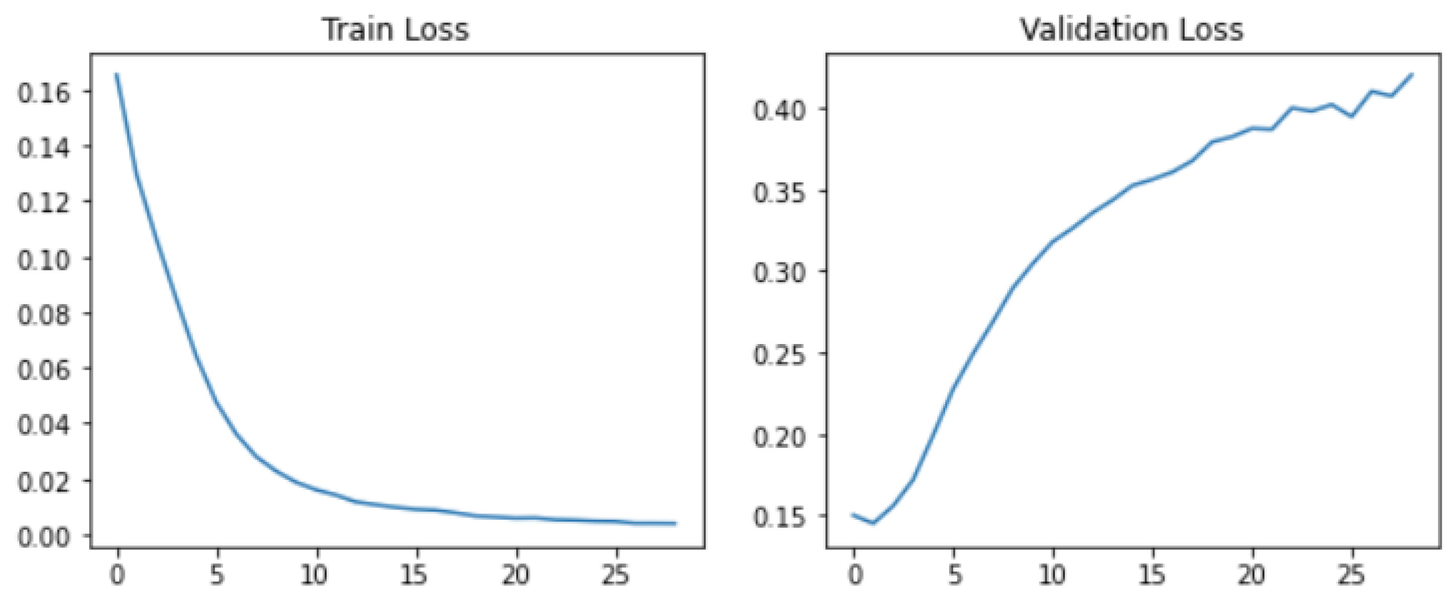
“After noticing the test accuracy tended to fluctuate randomly over 30 epochs, neither improving nor getting worse as training loss converged, and getting different patterns on different machines, we decided that the original model training process led to significant o v e r f i t t i n g on the train set, so we decided to implement an early-stoppage protocol in our analysis. This practice also let us analyze how quickly models would converge in terms of epochs.”
The e a r l y s t o p p i n g procedure allows stopping the training of a model when specified conditions are satisfied. In general, what early stopping does is simply to stop the training if there is no improvement in the validation loss for N. The choice of the value does usually depend on the slope of the loss when the phenomenon starts. If the loss is a steep upward curve, it is better to set N to a low number in order to avoid an extreme reduction of the model’s accuracy while if it is simply unstable, a large value is the right choice to allow the model to find its true path and not stop the training early without reasons.
However, in their source code there is no early stopping at all. Instead, the models are defined to be trained for 30 epochs whatever the behavior of the loss function. They decided to keep track of progress saving models every epoch. The way in which the algorithm is constructed allows one to evaluate the model through the test set at each epoch and save the metrics, hence after saving all the desired models related to specific epochs, they can simply confront the performances and decide what is their best model. In our opinion, this is the most critical part because they reported to reach the best metrics and best models thanks to the early stopping procedure, but, in reality, we cannot confirm their achievement in the way it was stated.
Since we wanted to try to reproduce their actual results claimed in the article and there really is an overfitting problem during training (Figure 4), we decided to implement a true early-stopping procedure. As Listing 6 shows, first of all, three variables need to be defined:
  • last_loss is just a random big enough value to initialize the procedure;
  • Patience is the previously cited number N that determine how many epochs there can be with no improvements;
  • trigger_times is another value that needs to be set equal to 0 at the start of the training and behaves like a flag. Every time there is an increase in the validation loss during an epoch, this number is increased by 1.
Listing 6. Early-Stopping Procedure.
Information 14 00076 i006
After that, we enter the for loop where the actual training begins. At the end of each epoch, the resulting losses are obtained and the validation one is kept for the procedure: there must be N consecutive epochs in which the loss does not decrease to stop the training, and the trigger_times variable keeps count of the times. If such a situation occurs, the resulting model will be the one at the current epoch even if the training is not finished. This is one of the simplest but most effective ways to prevent overfitting, and it is extremely commonly employed in deep learning algorithms.
The last thing that we wanted to highlight is another fundamental absence in the original source code. In reproducibility studies, we have to be sure that the results achieved can be re-obtained once the experiment is done by someone else at other times and through different devices. In Machine Learning, and more generally data science projects, it is useful to keep in mind that many random factors could affect the final outputs. One way to do address this is fixing the randomness of calculation with a function that is called random seed. The aim is to force the random processes to start at the same point every time, so in the splitting case, we would have the three subsets composed by the same data every time the experiment is initialized. Since data is divided in batches by a generator before the training, the generator exploits the pseudo-random calculus of the machine to create those batches and since there was no random_seed, at each run it creates different batches that lead to changes in the model’s training. Usually, it is one of the first procedures to be implemented in an experiment in order to avoid small fluctuations of results and to eliminate any hint of randomness. Below in Listing 7, it can be seen that a version of random seeding is implemented our code. The seed_value can be set to any number, it is not important which one, but once a number is chosen it always has to remain the same because it is the only way to follow the same order by which the pseudo-randomness starts.
Listing 7. Random-Seed Function.
Information 14 00076 i007
Even if we did implement the function, we decided to not use it since we do not know how they generated the batches or how many runs they did before classifying their results as reliable. A simpler method for ensuring a reliable result and reducing traces of randomness that does not exploit random_seed is to compute N different trials and then average the results, since the mean is known to recover outliers. Usually this process is called K-means cross-validation, and the dataset is split just once in K parts and subsequently, K 1 parts are exploited for the model’s training while the remaining part is used to evaluate the model. Then the training is performed K times, and each time a different section of the dataset is considered for the evaluation phase. In the end, the average of all the results is taken as the final result and this has a more reliable output compared to a single round of training-and-test.
In our case, the dataset is already divided and all the related published achievements used the original division. Hence, we cannot perform an actual K-means cross-validation. What we did in our study is to simply perform fine-tuning for each model 5 times and merge with the average every final result. The only thing that can change is how the data are divided in batches to feed the model due to the random split performed by the generator, so the losses and accuracy cannot highly diverge. However, this method provides more certainty in the final results.

5. Experimental Results

In this section, we go through the conclusions made by the authors of the article alongside our outcomes, and we discuss the differences found. This section is divided into five sections, each one related to a corresponding model. First, we will discuss the two basic versions of BERT and after that, the newer alternatives AlBERT, DistilBERT and RoBERTa.

5.1. A Note of Caution: Test Accuracy

Before starting with the comparisons, we want to focus on a fundamental issue in the evaluation approach proposed in the original paper during the model’s training. As we discussed earlier, there is no early-stopping in the source code even if this is described in the paper. As a consequence, the best result in the paper derives from a post-hoc analysis of the best test accuracy. Indeed, the approach employed was not based on the study of the progress of validation loss and the subsequent stop of training; instead, it merely consisted of an assessment of several models’ training and their related accuracy measures, assessing the best performance only by trial and error. In Figure 5, the declared losses and the corresponding accuracy are displayed for each model’s versions. We will show that the best performances in each model stated by the authors are just the peaks found in the bottom-right graph of the figure and do not follow any particular selection method.
This is not exactly the correct methodology for the training/validation/test approach in Machine Learning. In fact, one would:
  • Train the parameters of the model with the training set;
  • Optimize the hyper-parameters of the model with the validation set;
  • Select the model that obtains the best performance on the validation set;
  • Test the selected model on the test set.
In order to show the differences with the original paper, in the following section we will show test accuracy across the different epochs, keeping in mind that this would not be the correct approach.
After discussing the fundamental definitions for evaluating classification tasks (see for example Figure 6), for each model, we will present the following information:
  • A table with training times and test accuracy for 30 epochs and for a (supposedly) early-stopping approach (for example, Table 6a);
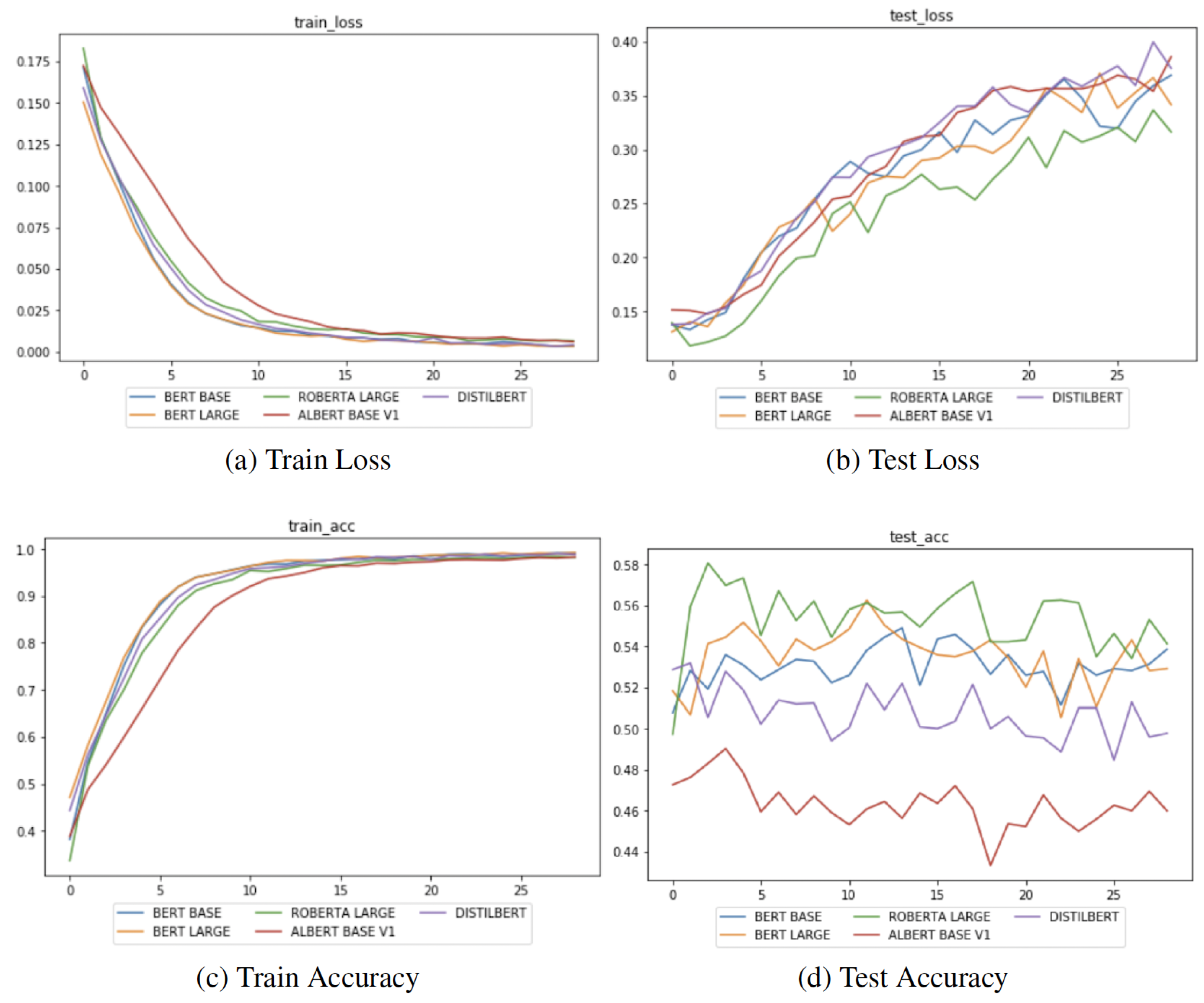
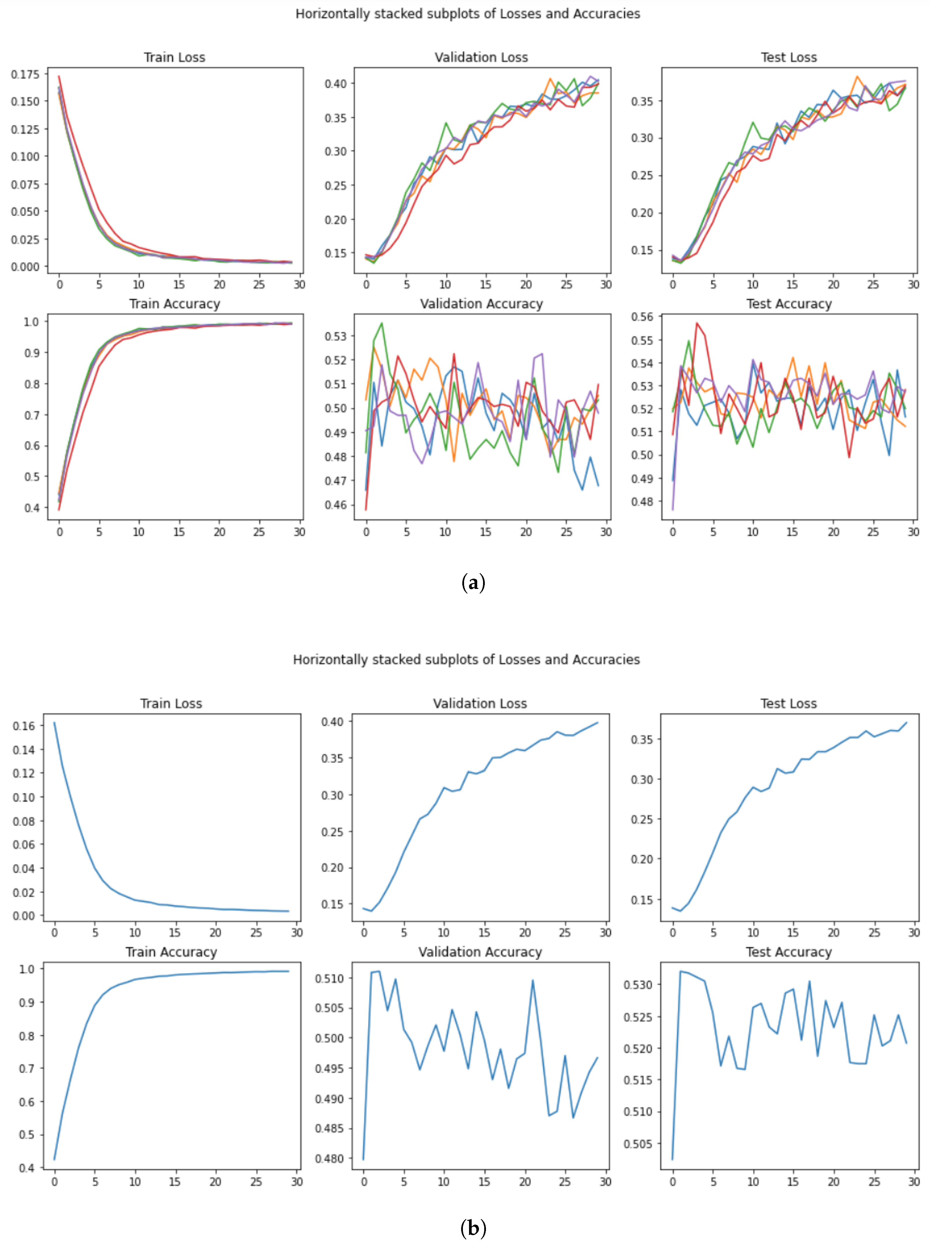
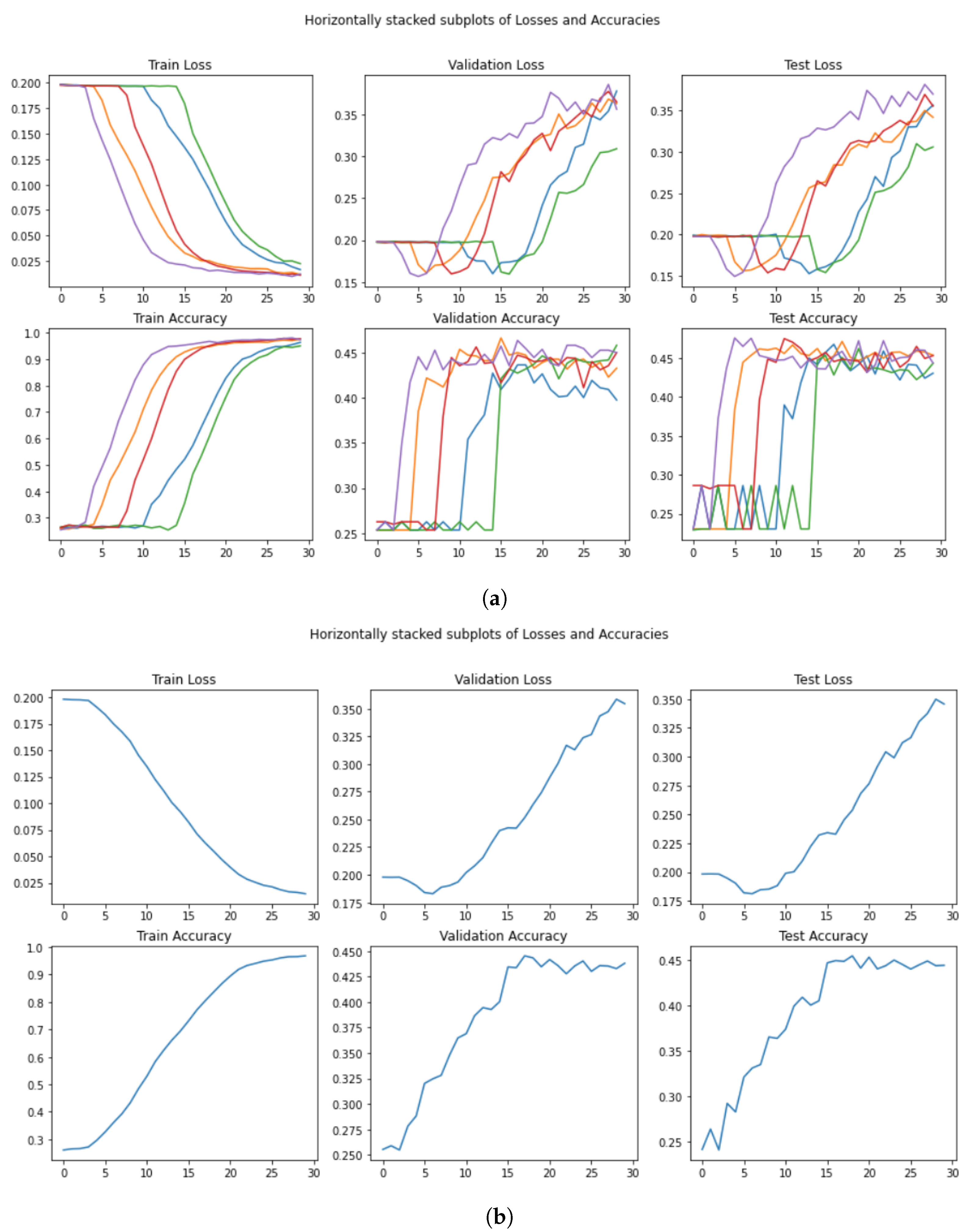
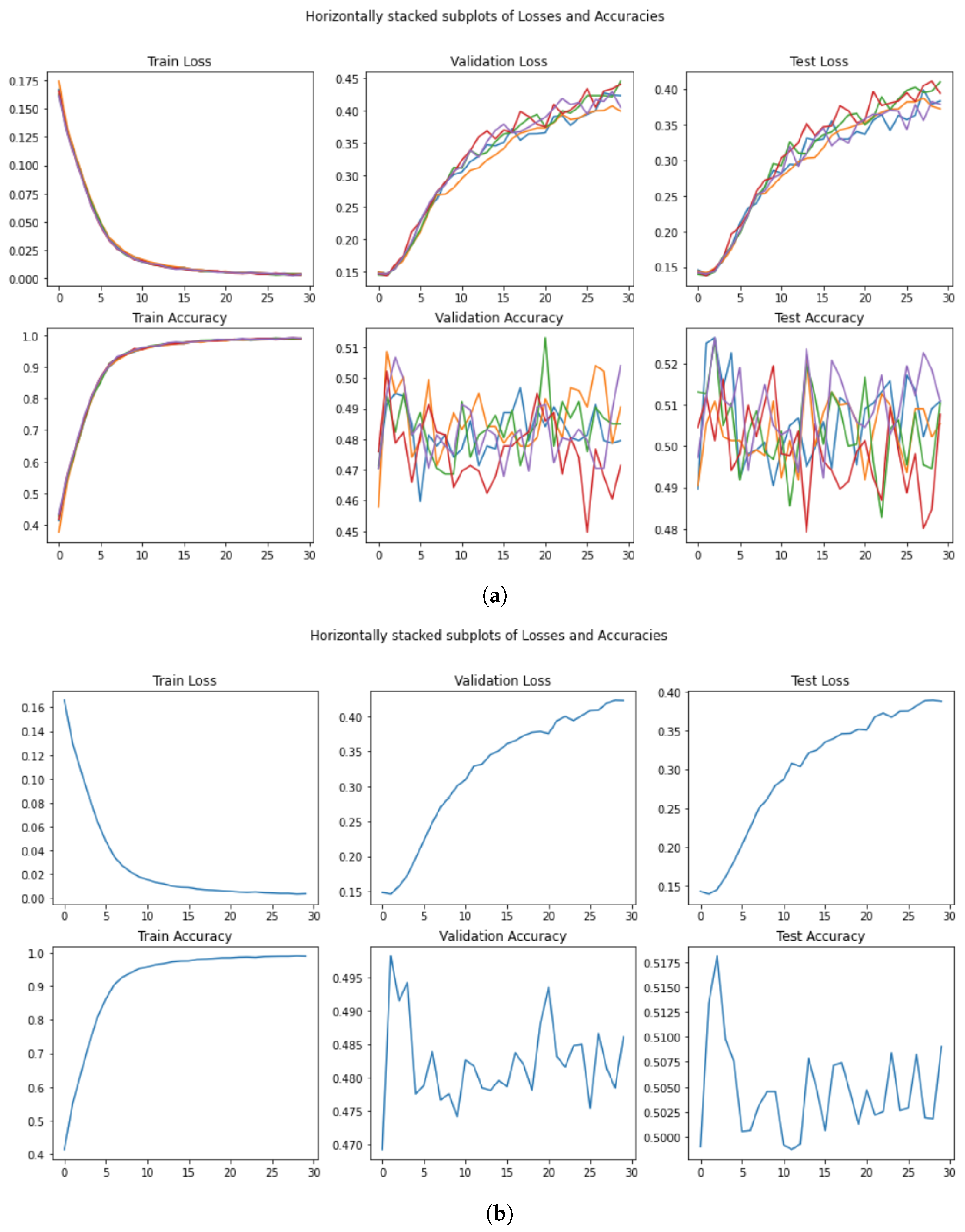
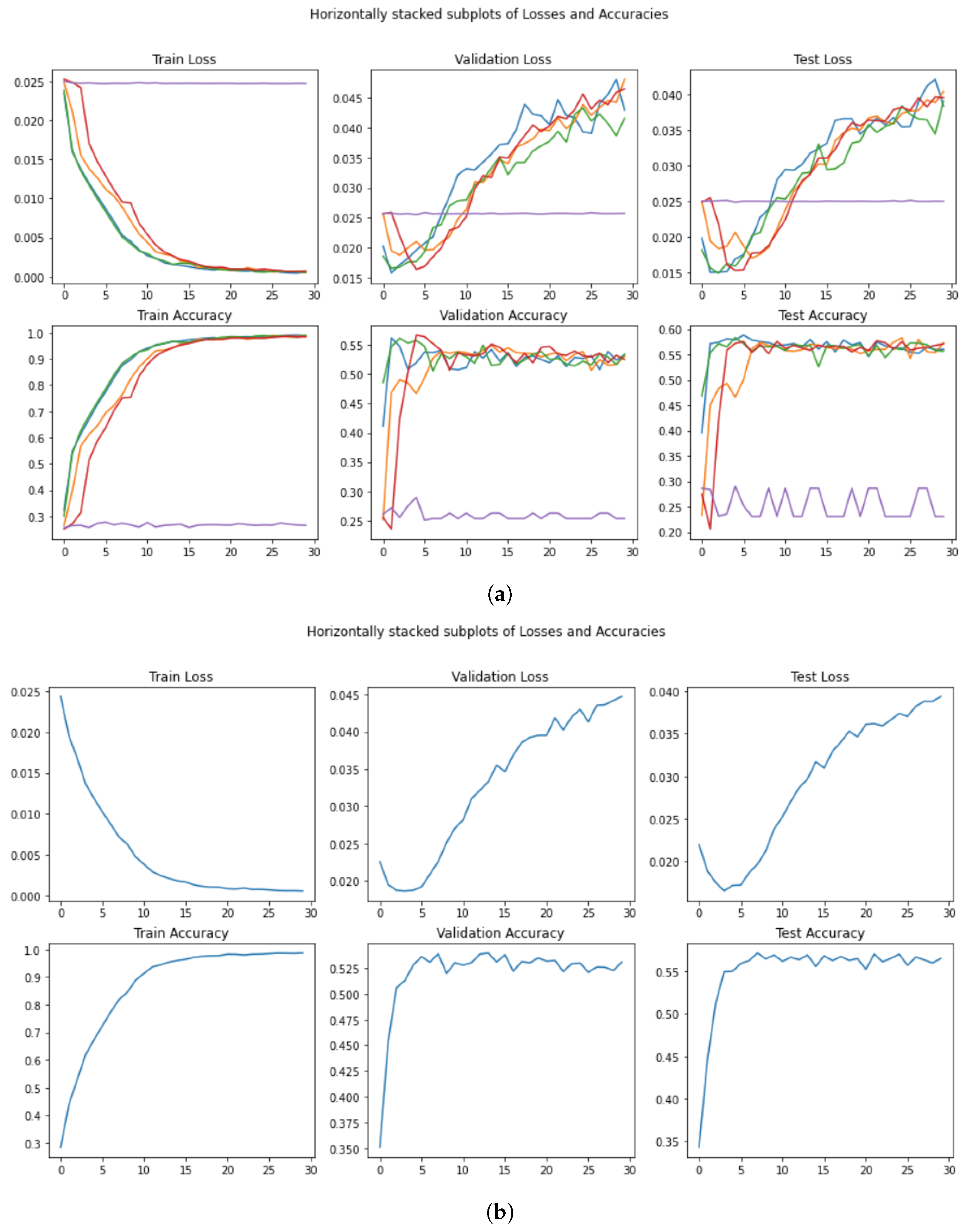
  • A Figure with training/validation/test loss and accuracy (for example, Figure 7a);
  • A Figure with the average training/validation/test loss and accuracy (for example, Figure 7b);
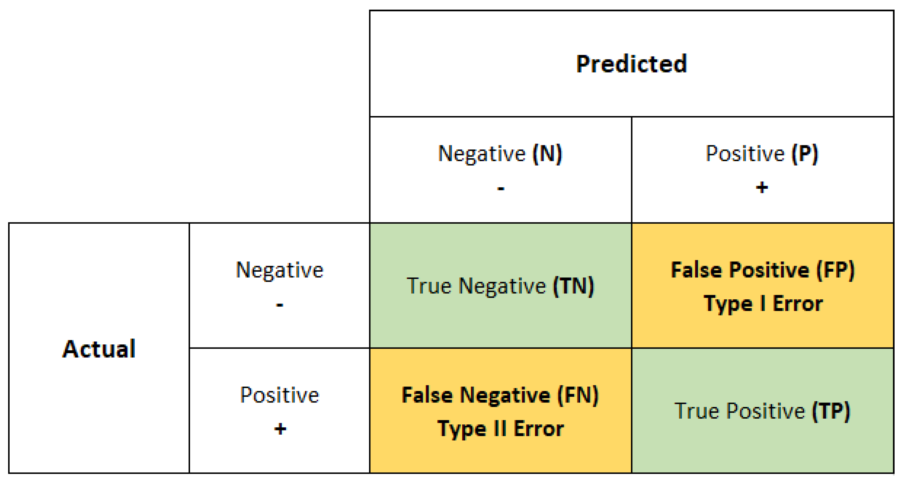
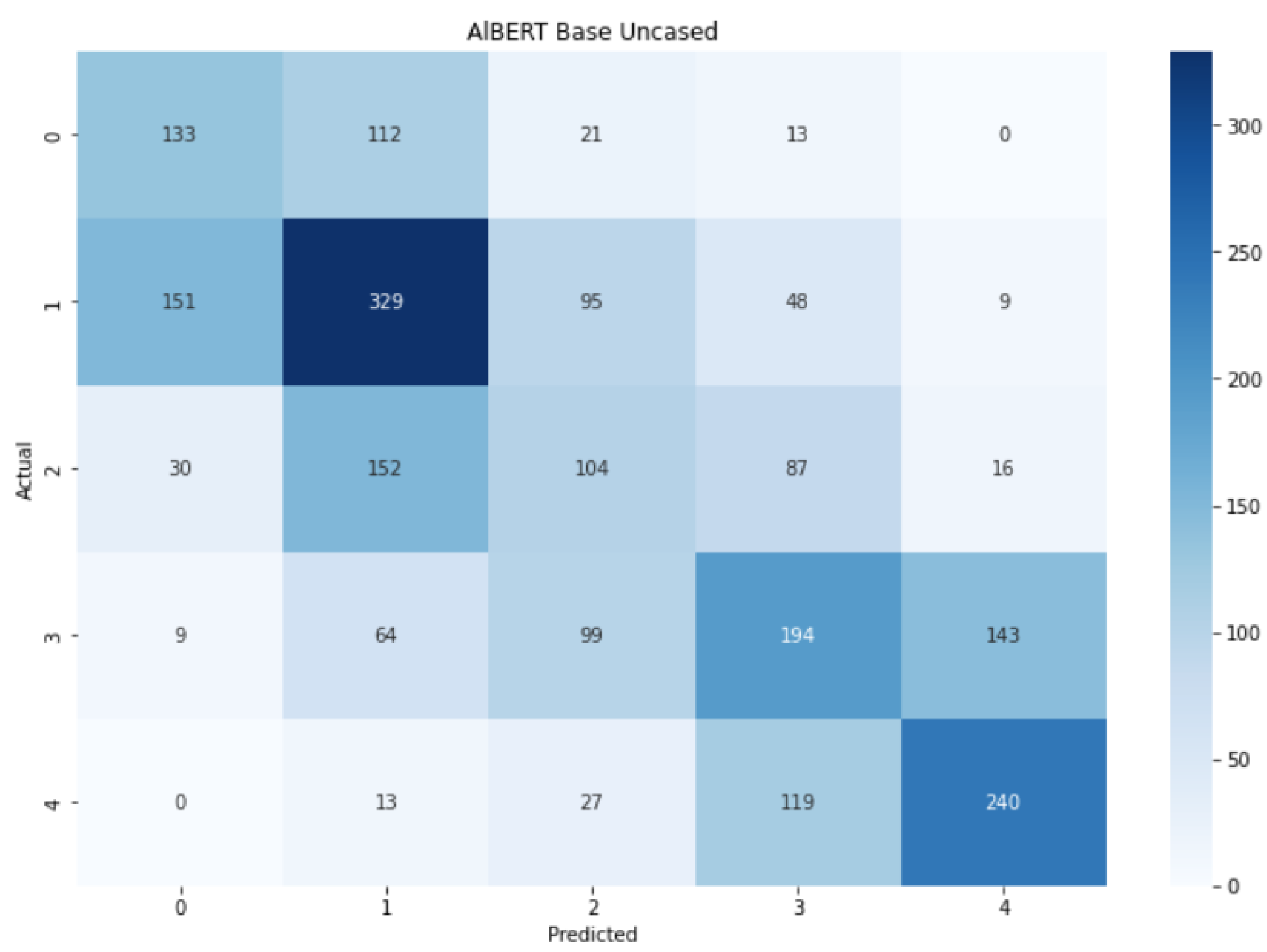
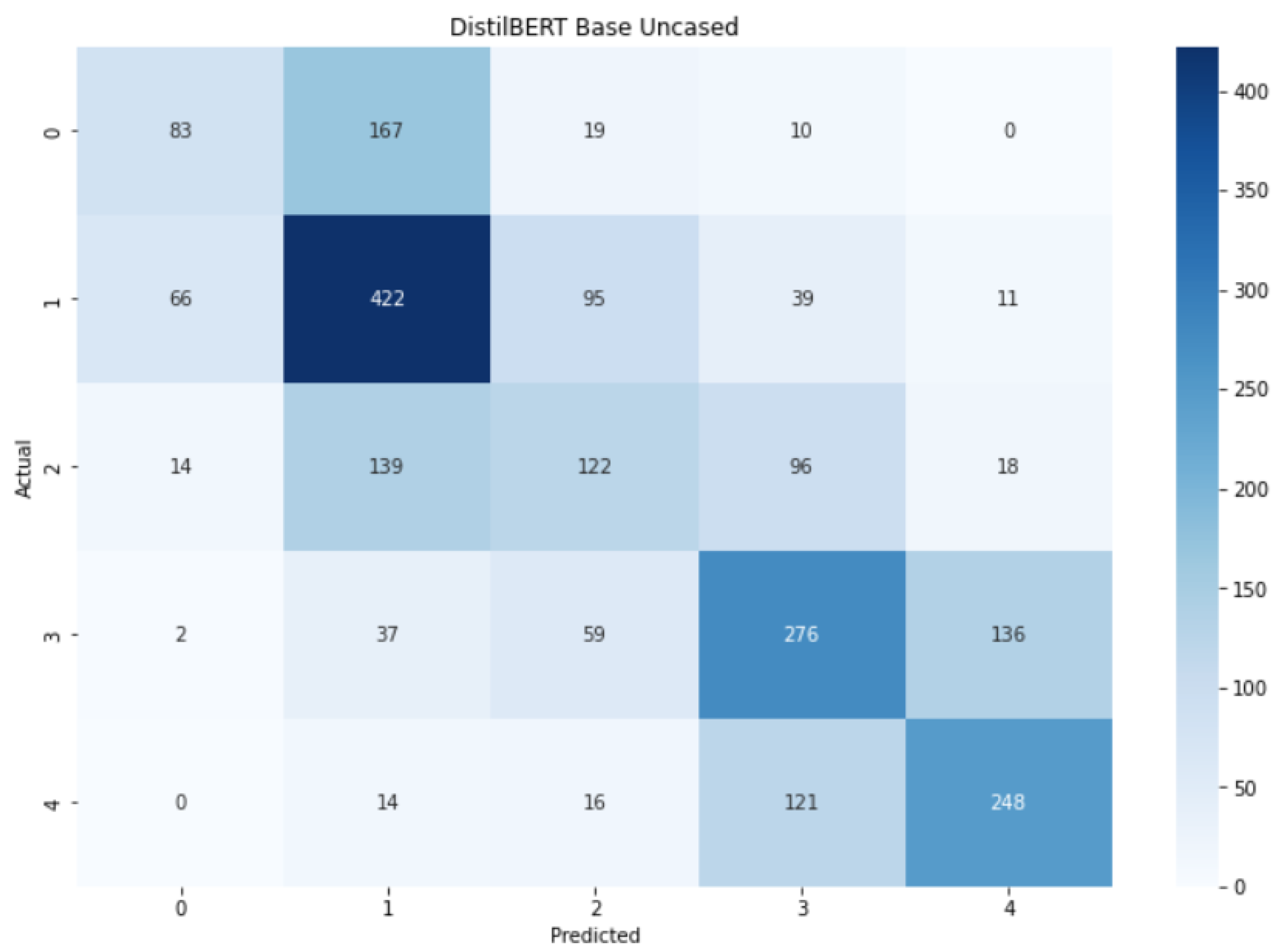
  • A Figure with the confusion matrix for the five classes (for example, Figure 8).

5.2. Evaluation Metrics

Based on the task at hand, several metrics and scores have to and can be considered. In classification tasks, our aim is to understand and calculate how many correct predictions the model makes. Indeed, since the data of the sentiment classification task are grouped into classes and the outcomes of the model are probabilities that correspond to the probability of being related to one category, we can only compare labels. In this way, we will have a situation in which some predictions are equal to the actual label and some predictions are wrong with respect to the actual category. For each class, those options are called t r u e p o s i t i v e and f a l s e p o s i t i v e . For instance, in binary classification we usually define a label as the positive output and the other category as the negative one. Hence, at the end of the prediction we are going to have four different categories: True Positive ( T P ), an outcome where the model correctly predicts the positive class, False Positive ( F P ), an outcome where the model incorrectly predicts the positive class, False Negative ( F N ), an outcome where the model incorrectly predicts the negative class, and True Negative ( T N ), an outcome where the model correctly predicts the negative class. The metric that collects and displays such distributions is called a confusion matrix (Figure 6). It helps to visualize how good the model’s prediction works and which class is predominant by the choices of the algorithm, if there is one, and based on the purpose of the research it allows rebalancing the model by managing the thresholds for probabilities, for example.
The four possible categories and the related distributions can be combined to obtain other measures that help to define the goodness of a model. In the original work, and in this paper, we use Accuracy as the proportion of the correct answers (TP + TN) compared to the total number of answers (TP + TN + FP + FN). In general, this measure is useful when all classes are of equal importance and the dataset is balanced, because if not, the accuracy for a class could be higher than for the other, leading to a misinterpretation of the overall performance of the model.

5.3. BERT_BASE

Our discussion about the experimental performances starts from the first published version of BERT architecture, i.e., the BERT BASE . The authors of the paper distinguished two main approaches. Since their work was partially also a reproducibility study, they first focused on the execution of all the 30 epochs for training and subsequently, they showed results for their so-called early-stopping procedure. We want to follow this pattern with the same type of approach.
The first aspect that we notice from Table 6a is the training time per epoch in minutes. The results are quite similar ( 5.38 their algorithm, 6 min our algorithm). There is a difference of few tens of seconds between the two, but we obtained the same order of magnitude, and hence we consider the results comparable. Although our GPU was, computationally speaking, more powerful, our run took more time to complete an epoch. This is probably due to the specific software used for the experiment, the package versions, and also the way in which the GPU was exploited. This is because even if a GPU is available, there are several techniques in which its usage can be optimized, and maybe they found a way to get the maximum capability out of their processor. These slight differences aside, we can state that the amount of time needed for the training of an epoch was reproduced.
The test accuracy after 30 epochs is stated in the article as 0.538 , while our average test accuracy is 1.7 % lower, that is 0.521 , which does not deviate much from the reported accuracy of 0.532 in the original paper [19]. Such a difference is very likely caused by a different random seed (as all the subsequent results) and therefore, their results could be a fortuitous case. For instance, if we observe the last subplot of Figure 7a, we can see how one of those five runs (red line) reaches a 0.530 value at the end of the 30 epochs. The expected accuracy (as the average of all the possible runs) is shown in Figure 7b. We can clearly observe a generic pattern in this figure: the trend starts with a low value but suddenly it reaches the peak of values, followed by a sharp decrease after a few epochs. Then, there is a slight increase again, characterized by a swinging and unclear movement and ending with the last small decrease. Comparing this with the remaining graphs in the same figure, it is obvious that the model suffers from overfitting.
This is a behavior also described by the authors, as we know, and it is the reason for the second approach. In the article they state:
“The performance did not peak until the 13th epoch and BERT BASE achieved a 0.549 accuracy on the SST-5 test set.”
If we take a look at Figure 7a, one run (the blue line) did actually reach its peak at the 13th epoch but, in any case, this does not represent the application of an early-stopping procedure. Indeed, if we observe the top-right panel in the same figure, it seems clear where the loss starts increasing heavily and where the optimization (validation phase) should stop.
Instead, if we perform a correct training/validation procedure, we would choose the optimal model after two epochs of the validation phase, and obtain a test accuracy of 0.532 .
The last thing that we want to show is the confusion matrix related to the accuracy obtained with the early stopping procedure. Although the accuracy reached was not like the one stated in the article, it achieved the same value of the original result, and in Figure 8 the predictions in relation with the actual labels can be seen, and also how the model can identify the differences between the categories rather well. The dark diagonal means that, in general, positive sentences are predicted correctly and the same is true for the negative sentences. There are some confusions between near classes, such as 0 and 1 or 3 and 4, but most of them are correctly classified. The opposite labels are well-differentiated, meaning that negative and positive words are identified excellently.

5.4. BERT_LARGE

The second model analyzed in the article was BERT LARGE . Table 6b reports the values we obtained and, since for this model we were forced to use Colab Pro and its premium GPUs, the training time cannot be comparable. Indeed, there is an extreme difference between the two values. For instance, we can notice that the amount of time required for our training is practically equal to the one required for the AlBERT model training, which has 300 M fewer parameters than BERT LARGE .
Focusing on the accuracy measures reported in the table, we can clearly see the similarities inside the second column, i.e., the 30 epoch results. Our measure, collected by averaging the five-run results, is comparable to the one observed in the article. However, a larger difference can be seen when we consider the early-stopping procedure. The authors stated a value of 0.562 , but in this case, too, there is no connection between the value and the trend of the related loss. In Figure 9a, there is one run (orange line), which shows the accuracy of 0.562 at the 12th epoch. However, it is ten epochs away from the lowest loss, the point in which theoretically the model performs at best.
Furthermore, during the training, we encountered some difficulties due to unexpected behavior of the model and its losses. Figure 9a displays the 5 runs revealing how some runs (two in our case) failed to converge and instead caused stationary behavior in which the losses stay around 0.2 and the accuracy stays between 0.2 and 0.3 . We tried to repeat the same test multiple times and we always found the same behavior despite the different initial starting point of the generator. It seems that in certain runs, the model fails to reach a converging point, leading to the stationary status.
For this reason, we decided to study the average performance without the non-converging ones. Indeed, in Figure 9b, the value reached with the early-stopping procedure is 0.441 , a value too low to be considered comparable with the one published.
Lastly, Figure 10 reports the confusion matrix on the test data. As for BERT BASE , the matrix shows three macro squares that characterize how the model fails to predict the correct label. Strongly negative and strongly positive sentiments were mis-categorized as weakly negative and weakly positive sentiments, respectively, roughly half the time. Neutral sentiments were mis-categorized as weakly negative roughly half the time as well. Despite these patterns, the diagonal is tighter than the one in the BASE version of BERT, meaning that overall the model performs slightly better, a fact that, of course, is also highlighted by the higher accuracy value.

5.5. AlBERT

The first alternative of BERT that was studied in the article is AlBERT. With this architecture, we have a decrease of almost 2 min in the time required for an epoch to be completed with respect to BERT BASE , as shown in Table 6c. However, between the experiment run by the authors of the paper and ours, there is a gap of one minute, in accordance with the trend of all the experiments, where our training time is always a bit greater than the one required by them, but both results are in the same order of magnitude.
Through our five runs (Figure 11a), we can notice a general pattern. Each run has a different point (number of epochs) when the loss starts to decrease.
The averaged scores (Figure 11b) show that this model requires between 15 and 20 epochs to reach its peak in the validation set.
As stated in the original article, AlBERT performed far worse than expected on the SST-5 dataset. Since it was not part of their reproducibility study, the authors immediately used the early-stopping procedure, considering only the best test accuracy obtained. In any case, we were never able to reproduce that score and, given a correct validation procedure, the best score obtained was 0.453 .
However, it is the worst BERT model in terms of performance accuracy and this reduction likely outweighs the benefits of the decrease in training time, and therefore the utility of AlBERT on novel fine-grained NLP tasks is in question.
Figure 12 displays the confusion matrix related to the AlBERT model and, despite the lowest accuracy value, we can clearly see the distinction between positive and negative labels, shwoing that the model is able to understand such a difference. Nevertheless, it struggles to identify the right label when confronting extreme sentiment, for instance between 0 and 1, where the number of errors increased. Finally, one last thing could be observed: in the center there is a darker square that shows how the neutral sentences can be difficult to be correctly classified and that they can often be recognized as weak sentiments.

5.6. DistilBERT_BASE

DistilBERT BASE is the second alternative of BERT considered in the analysis. Lighter and faster than BERT BASE , its aim is to provide a choice that requires less training time at the expense of a small loss in terms of performance accuracy by the exploitation of the distillation technique. The goal, indeed, is reached quite well, with only 2.54 min per epoch in the pivotal experiment and 2.57 in our experiment (Table 6d), and a gap of just 1% in test accuracy between the two approaches. Furthermore, the model also requires less training time than AlBERT but it performs far better than the previous alternative, and is the fastest to train of all the models tested.
Regarding reproducibility, as in the AlBERT case, the authors of the article did not declare the performance achieved after the entire training (30 epochs), and hence we cannot compare our result of 0.509 . Instead, their best score reaches the 0.532 value during the second epoch, complying with the overfitting behavior, visible in Figure 13a in the purple line. In this case, it is it not easy to see a pattern across the five runs. However, Figure 13b helped us find a more specific pattern. The best expected value in the validation phase occurs after a few epochs in the validation step. Consequently, the best value for DistilBERT BASE is equal to 0.518 , discovered in the third epoch.
The pattern shown by the confusion matrix for DistilBERT BASE (Figure 14) is very similar to the ones for BERT BASE and AlBERT. The extreme labels and the central labels form 3 intersecting clusters in which the labels can be identified as other classes existing in the current cluster. Despite this situation, there is still a darker diagonal that implies an overall correct prediction through all the classes, with peaks in labels 1, 3, and 4.

5.7. RoBERTa LARGE

The last model and alternative analyzed is the one that, according to the authors of the paper, reached the state of the art on fine-grained sentiment classification, RoBERTa LARGE (see Table 6e). It is the largest model in terms of the number of parameters among the 5 models considered in the experiment. The training times between our reproduced experiment and the original one cannot be compared because, firstly, in the article there is no statement regarding training time, and secondly because we used the GPUs of Google Colab.
In the original paper, we have only the accuracy value related to the early-stopping procedure. In addition, we wanted to highlight an inconsistency that we found in Figure 5: if we observe the line that represents the results of RoBERTa LARGE (the green line), there is no epoch in which the line reaches 0.602 . Instead, the maximum score we can read is around 0.58 . We do not know if the plot is an old version with a previous value, but we have to consider this fact an error or an inconsistency with regards to what is stated in the paper and what we can read from the figure.
In this sense, the result achieved in our experiments (see Figure 15a,b), showing an accuracy on the test set of 0.575 , is comparable to the number that we can see in the original figure. As an additional comment, we want to highlight the fact that even with a 30-epoch training, our RoBERTa LARGE outperforms all the other models exploited in the experiment, with an accuracy score of 0.565 . Moreover, also with this model, we witnessed abnormal stationary behavior identical to what was found for BERT LARGE .
In Figure 16, the last confusion matrix is shown. The main difference between this figure and the rest of the matrices shown is that while there are still the two macro areas for the extreme sentiments, when dealing with the more neutral part, there is not a big square anymore. Instead, we can distinguish two smaller squares that intersect on the neutral label, meaning that the model can recognize weakly positive and weakly negative in a more efficient way. However, RoBERTa LARGE also confuses extreme sentiment with weak sentiment in a significant way, exactly like BERT LARGE .

6. Discussion

In this section, we summarize the main insights that were derived after the whole experimental analysis, and we will try to answer the following questions.

6.1. How Does This Study Reflect on Current Knowledge about Issues in the Reproducibility of Computational Experiments?

In Section 1, we have seen how the research community has (slowly) increased its interest in issues concerning reproducibility. In particular, after the article published in Nature in 2016, the effort that researchers have put into understanding the relevant limits has extended and spread through the entire research field. There is still a very active community in NLP and IR that carries on with the idea of standard experimental analysis by means of international forums and shared tasks.
In our opinion, there are some fundamental steps that need to be made by researchers in order to improve experimental analysis and, ultimately, make progress in science. In this sense, we share the ideas discussed by [36], and we believe that there are some necessary best practices regarding choice of data, source code, models, experimental setting, and analysis that should be documented in any research paper that presents experimental results.

6.2. Was the Original Study by Cheang Et Alii Able to Provide All the Necessary Information to Ensure Its Reproduction in All Respects?

The original paper has the merit of following some of the aforementioned best practices: the choice of a standard benchmark used in NLP, the publication of the source code, and the use of notebook files, i.e, a partial explanation of the experimental environment. Beyond some syntax errors that had to be fixed due to a difference in the version of the packages (something that was missing in the original paper), the source code ran without any difficulty.

6.3. What Are the Problems and Challenges Encountered?

Despite the fact that we were able to run the code with minor bug fixes related to software version, we found some major limitations: First, the inconsistency between the documented stopping criterion in the paper that was not implemented in the code; second, the absence of an initial random seed in order to reproduce “randomness” exactly in the source code [35]; third, a better description of the hardware used (CPUs and RAM, in particular), all of which could have helped us to understand the differences in running time execution.
Besides these issues, we encountered a major flaw in the evaluation approach that was, on the other hand, very interesting by way of shedding light on some common pitfalls in the development cycle of machine learning optimization [37].

6.4. What Could Be Done in the Original Study to Overcome the Problems Found?

We believe that only a better documentation, both in the research paper and in the source code, could overcome most (if not all) the issues we encountered in this reproducibility study. The best practices suggested by [36] are one of the best starting points for a checklist of all the things a researcher should take into account “before” any experimental analysis. In order to mitigate issues like the ones related to the stopping criterion (an approach that is described in the paper but that is missing in the code), we believe that only a more accurate check on all the steps is the solution. In this sense, a better use of the notebooks could help in reducing the probability of these kinds of errors [38].

7. Conclusions

In this paper, we described a thorough reproducibility study of a sentiment classification task experiment. By means of an analysis of the paper “Language Representation Models for Fine-Grained Sentiment Classification”, written by Cheang et al. (2020), the main set of rules that has to be considered when performing an experiment was discussed. Reproducing a study conducted by other researchers can be a very difficult task. There are several aspects to a project, and each of them must be considered, analyzed, and reproduced in a correct manner. Furthermore, whoever performs the original experiment should also take into account these aspects in order to allow everyone to reproduce their work. Moreover, the act of reproducing an experiment can be seen as the verification of its validity and, in this sense, studies have to be conducted in the most reliable way possible.
During our work, we encountered a few issues, starting with the creation of a similar environment to the one used by the authors of the article, but also understanding the source code and fixing some syntactic errors, and finally being able to reproduce the work with comparable results.
First of all, we had to set up the experimental environment. The original article did not contain any information regarding the environment, apart from the series number of the GPU hardware, and lacked a list of packages, libraries, and software used. Fortunately, we had a GPU at our disposal and, furthermore, it was very similar to theirs, allowing us to have quite comparable results in terms of processing time. On the other hand, we had to decide on other details about the settings that inevitably could lead to some minor differences in the outcomes.
Regarding the source code, after fixing some minor syntax errors, we went through the analysis of some inconsistencies between the paper and the source code. The most ‘interesting’ inconsistency was the missing implementation of the early-stopping procedure. The authors designed the experimental analysis in a way to have access to test accuracy scores after each epoch, and hence, they were able to keep the best value obtained even if there was no validation step to support such a score. In our experiments, we tried to perform a set of repeated experiments and could see what epoch, on average, could be the optimal one in the validation phase. Finally, after collecting and analyzing all the necessary evaluation measurements, our final scores differ from the original values by almost 2 percentage points.

Author Contributions

Conceptualization, G.M.D.N. and R.M.; methodology, G.M.D.N. and R.M.; software, G.M.D.N. and R.M.; investigation, G.M.D.N. and R.M.; writing—original draft preparation, G.M.D.N. and R.M.; writing—review and editing, G.M.D.N. and R.M. All authors have read and agreed to the published version of the manuscript.

Funding

This research received no external funding.

Data Availability Statement

All the source code that has been used to produce the results for the analysis is freely available at the following link https://github.com/riccardominzoni/reproducibilitycasestudy (accessed on 19 January 2023).

Conflicts of Interest

The authors declare no conflict of interest.

References

  1. Pugliese, R.; Regondi, S.; Marini, R. Machine learning-based approach: Global trends, research directions, and regulatory standpoints. Data Sci. Manag. 2021, 4, 19–29. [Google Scholar] [CrossRef]
  2. Baker, M. Reproducibility crisis. Nature 2016, 533, 353–366. [Google Scholar]
  3. Lastra-Díaz, J.J.; García-Serrano, A.; Batet, M.; Fernández, M.; Chirigati, F. HESML: A scalable ontology-based semantic similarity measures library with a set of reproducible experiments and a replication dataset. Inf. Syst. 2017, 66, 97–118. [Google Scholar] [CrossRef]
  4. Crane, M. Questionable Answers in Question Answering Research: Reproducibility and Variability of Published Results. Trans. Assoc. Comput. Linguist. 2018, 6, 241–252. [Google Scholar] [CrossRef] [Green Version]
  5. Yu, B.; Hu, X. Toward Training and Assessing Reproducible Data Analysis in Data Science Education. Data Intell. 2019, 1, 381–392. [Google Scholar] [CrossRef]
  6. Cockburn, A.; Dragicevic, P.; Besançon, L.; Gutwin, C. Threats of a replication crisis in empirical computer science. Commun. ACM 2020, 63, 70–79. [Google Scholar] [CrossRef]
  7. Daoudi, N.; Allix, K.; Bissyandé, T.F.; Klein, J. Lessons Learnt on Reproducibility in Machine Learning Based Android Malware Detection. Empir. Softw. Eng. 2021, 26, 74. [Google Scholar] [CrossRef]
  8. Gundersen, O.E.; Shamsaliei, S.; Isdahl, R.J. Do machine learning platforms provide out-of-the-box reproducibility? Future Gener. Comput. Syst. 2022, 126, 34–47. [Google Scholar] [CrossRef]
  9. Reveilhac, M.; Schneider, G. Replicable semi-supervised approaches to state-of-the-art stance detection of tweets. Inf. Process. Manag. 2023, 60, 103199. [Google Scholar] [CrossRef]
  10. Pineau, J.; Vincent-Lamarre, P.; Sinha, K.; Larivière, V.; Beygelzimer, A.; d’Alché Buc, F.; Fox, E.; Larochelle, H. Improving reproducibility in machine learning research: A report from the NeurIPS 2019 reproducibility program. J. Mach. Learn. Res. 2021, 22, 1–20. [Google Scholar]
  11. Cheang, B.; Wei, B.; Kogan, D.; Qiu, H.; Ahmed, M. Language representation models for fine-grained sentiment classification. arXiv 2020, arXiv:2005.13619. [Google Scholar]
  12. Wankhade, M.; Rao, A.C.S.; Kulkarni, C. A survey on sentiment analysis methods, applications, and challenges. Artif. Intell. Rev. 2022, 55, 5731–5780. [Google Scholar] [CrossRef]
  13. Devlin, J.; Chang, M.W.; Lee, K.; Toutanova, K. Bert: Pre-training of deep bidirectional transformers for language understanding. arXiv 2018, arXiv:1810.04805. [Google Scholar]
  14. Rougier, N.P.; Hinsen, K.; Alexandre, F.; Arildsen, T.; Barba, L.A.; Benureau, F.C.; Brown, C.T.; De Buyl, P.; Caglayan, O.; Davison, A.P.; et al. Sustainable computational science: The ReScience initiative. PeerJ Comput. Sci. 2017, 3, e142. [Google Scholar] [CrossRef] [Green Version]
  15. Wieling, M.; Rawee, J.; van Noord, G. Reproducibility in computational linguistics: Are we willing to share? Comput. Linguist. 2018, 44, 641–649. [Google Scholar] [CrossRef]
  16. Whitaker, K. The MT Reproducibility Checklist. Presented at the Open Science in Practice Summer School. 2017. Available online: https://openworking.wordpress.com/2017/10/14/open-science-in-practice-summer-school-report/ (accessed on 19 January 2023).
  17. Belz, A.; Agarwal, S.; Shimorina, A.; Reiter, E. A systematic review of reproducibility research in natural language processing. arXiv 2021, arXiv:2103.07929. [Google Scholar]
  18. Joint Committee for Guides in Metrology. International vocabulary of metrology—Basic and general concepts and associated terms (VIM). VIM3 Int. Vocab. Metrol. 2008, 3, 104. [Google Scholar]
  19. Munikar, M.; Shakya, S.; Shrestha, A. Fine-grained sentiment classification using BERT. In Proceedings of the 2019 Artificial Intelligence for Transforming Business and Society (AITB), Kathmandu, Nepal, 5 November 2019; Volume 1, pp. 1–5. [Google Scholar]
  20. Lan, Z.; Chen, M.; Goodman, S.; Gimpel, K.; Sharma, P.; Soricut, R. Albert: A lite bert for self-supervised learning of language representations. arXiv 2019, arXiv:1909.11942. [Google Scholar]
  21. Sanh, V.; Debut, L.; Chaumond, J.; Wolf, T. DistilBERT, a distilled version of BERT: Smaller, faster, cheaper and lighter. arXiv 2019, arXiv:1910.01108. [Google Scholar]
  22. Liu, Y.; Ott, M.; Goyal, N.; Du, J.; Joshi, M.; Chen, D.; Levy, O.; Lewis, M.; Zettlemoyer, L.; Stoyanov, V. Roberta: A robustly optimized bert pretraining approach. arXiv 2019, arXiv:1907.11692. [Google Scholar]
  23. Aßenmacher, M.; Heumann, C. On the comparability of Pre-trained Language Models. arXiv 2020, arXiv:2001.00781. [Google Scholar]
  24. Socher, R.; Perelygin, A.; Wu, J.; Chuang, J.; Manning, C.D.; Ng, A.Y.; Potts, C. Recursive deep models for semantic compositionality over a sentiment treebank. In Proceedings of the 2013 Conference on Empirical Methods in Natural Language Processing, Seattle, WA, USA, 18–21 October 2013; pp. 1631–1642. [Google Scholar]
  25. Pang, B.; Lee, L. Seeing stars: Exploiting class relationships for sentiment categorization with respect to rating scales. arXiv 2005, arXiv:cs/0506075. [Google Scholar]
  26. Klein, D.; Manning, C.D. Accurate unlexicalized parsing. In Proceedings of the 41st Annual Meeting of the Association for Computational Linguistics, Sapporo, Japan, 7–12 July 2003; pp. 423–430. [Google Scholar]
  27. Lin, T.; Wang, Y.; Liu, X.; Qiu, X. A survey of transformers. AI Open 2022, 3, 111–132. [Google Scholar] [CrossRef]
  28. Vaswani, A.; Shazeer, N.; Parmar, N.; Uszkoreit, J.; Jones, L.; Gomez, A.N.; Kaiser, Ł.; Polosukhin, I. Attention is all you need. In Advances in Neural Information Processing Systems; Curran Associates, Inc.: Red Hook, NY, USA, 2017; Volume 30. [Google Scholar]
  29. Vaswani, A.; Shazeer, N.; Parmar, N.; Uszkoreit, J.; Jones, L.; Gomez, A.N.; Kaiser, L.; Polosukhin, I. Attention Is All You Need. arXiv 2017, arXiv:1706.03762. [Google Scholar]
  30. Wu, Y.; Schuster, M.; Chen, Z.; Le, Q.V.; Norouzi, M.; Macherey, W.; Krikun, M.; Cao, Y.; Gao, Q.; Macherey, K.; et al. Google’s Neural Machine Translation System: Bridging the Gap between Human and Machine Translation. arXiv 2016, arXiv:1609.08144. [Google Scholar]
  31. Wan, Z.; Xu, C.; Suominen, H. Enhancing Clinical Information Extraction with Transferred Contextual Embeddings. arXiv 2021, arXiv:2109.07243. [Google Scholar]
  32. Balagopalan, A.; Eyre, B.; Robin, J.; Rudzicz, F.; Novikova, J. Comparing Pre-trained and Feature-Based Models for Prediction of Alzheimer’s Disease Based on Speech. Front. Aging Neurosci. 2021, 13, 635945. [Google Scholar] [CrossRef] [PubMed]
  33. Zhu, Y.; Kiros, R.; Zemel, R.; Salakhutdinov, R.; Urtasun, R.; Torralba, A.; Fidler, S. Aligning Books and Movies: Towards Story-like Visual Explanations by Watching Movies and Reading Books. arXiv 2015, arXiv:1506.06724. [Google Scholar]
  34. Kingma, D.P.; Ba, J. Adam: A method for stochastic optimization. arXiv 2014, arXiv:1412.6980. [Google Scholar]
  35. Radford, A.; Narasimhan, K.; Salimans, T.; Sutskever, I. Improving Language Understanding with Unsupervised Learning; Technical Report; OpenAI: San Francisco, CA, USA, 2018. [Google Scholar]
  36. Ulmer, D.; Bassignana, E.; Müller-Eberstein, M.; Varab, D.; Zhang, M.; van der Goot, R.; Hardmeier, C.; Plank, B. Experimental Standards for Deep Learning in Natural Language Processing Research. arXiv 2022, arXiv:2204.06251. [Google Scholar]
  37. Biderman, S.; Scheirer, W.J. Pitfalls in Machine Learning Research: Reexamining the Development Cycle. arXiv 2021, arXiv:2011.02832. [Google Scholar]
  38. Skripchuk, J.; Shi, Y.; Price, T. Identifying Common Errors in Open-Ended Machine Learning Projects. In Proceedings of the the 53rd ACM Technical Symposium on Computer Science Education, SIGCSE 2022, Providence, RI, USA, 3–5 March 2022; Association for Computing Machinery: New York, NY, USA, 2022; Volume 1, pp. 216–222. [Google Scholar] [CrossRef]
Figure 1. Sample sentiment tree from SST-5 (figure from the original paper [11]).
Information 14 00076 g001
Figure 2. Model Architecture of Transformer (figure adapted from [29]).
Information 14 00076 g002
Figure 3. BERT input representation (figure adapted from [31]).
Information 14 00076 g003
Figure 4. Overfitting behavior through losses in DistilBERT.
Information 14 00076 g004
Figure 5. Plots of case study loss and accuracy per epoch for the 5 comparison models (figure adapted from the original work [11]).
Information 14 00076 g005
Figure 6. Confusion matrix for binary classification.
Information 14 00076 g006
Figure 7. Performance in the training, validation, and test set for BERT BASE . (a) Loss and Accuracy per run and per epoch. (b) Mean loss and mean Accuracy per epoch.
Information 14 00076 g007
Figure 8. Confusion matrix for BERT BASE .
Information 14 00076 g008
Figure 9. Performance in the training, validation, and test set for BERT LARGE . (a) Loss and Accuracy per run and per epoch. (b) Mean loss and mean Accuracy per epoch after non-converging runs are removed.
Information 14 00076 g009
Figure 10. Confusion matrix for BERT LARGE .
Information 14 00076 g010
Figure 11. Performance in the training, validation, and test set for AlBERT. (a) Loss and Accuracy per run and per epoch. (b) Mean loss and mean Accuracy per epoch.
Information 14 00076 g011
Figure 12. Confusion matrix for AlBERT.
Information 14 00076 g012
Figure 13. Performance in the training, validation, and test set for in DistilBERT BASE . (a) Loss and Accuracy per run and per epoch. (b) Mean loss and mean Accuracy per epoch.
Information 14 00076 g013
Figure 14. Confusion matrix for DistilBERT BASE .
Information 14 00076 g014
Figure 15. Performance in the training, validation, and test set for RoBERTa LARGE . (a) Loss and Accuracy per run and per epoch. (b) Mean loss and mean Accuracy per epoch after non-converging runs are removed.
Information 14 00076 g015
Figure 16. Confusion matrix for RoBERTa LARGE .
Information 14 00076 g016
Table 1. Overview of the latest research on reproducibility issues.
ReferenceYearMain Objective, Issues, and Results
[3]2017Library of semantic similarity measures publicly available for the first time, together with a set of reproducible experiments.
[4]2018A number of controllable environment settings that often go unreported can cause irreproducibility of results as presented in the literature
[5]2019Investigating students’ skills and understanding of reproducibility, whether they are able to communicate reproducible data analysis.
[6]2020Issues relating to the use of null hypothesis significance and discussion on alternative ways to analyze data and present evidence for hypothesized effects.
[7]2021A complete reproduction of five models and insights on the implications around the guesswork that may be required to finalize a working implementation.
[8]2022A survey of machine learning platforms to study whether they provide features that simplify making experiments reproducible out-of-the-box.
[9]2023A methodological approach for a replicable experimental analysis and a workflow using existing tools that can be transposed to other domains.
Table 2. Whitaker’s definitions of R-Terms [16] (table adapted from [17]).
Data
SameDifferent
CodeSameReproducibleReplicable
DifferentRobustGeneralisable
Table 3. SST-5 label distribution.
SetLabel 1Label 2Label 3Label 4Label 5Total
Training109222181624232212888544
Validation1392892292791651101
Test2796333895103992210
Table 4. Model Comparison (table adapted from [11]).
ModelNo. LayersNo. Hidden UnitsNo. Self-Attention Heads
(Total Trainable Parameters)
BERT BASE 1276812
(110 M)
BERT LARGE 24102416
(340 M)
AlBERT BASE 1276812
(12 M)
DistilBERT BASE 676812
(66 M)
RoBERTa BASE 1276812
(125 M)
RoBERTa LARGE 24102416
(355 M)
Table 5. A summary of the environment used by the original paper and the reproduced experiment. The version of Python and Jupyter notebook of the original paper were deduced by the date of the submission of the paper and the date of the source code uploaded on GitHub.
ItemOriginal PaperOur Experiment
GPUNVIDIA GeForce GTX 1080NVIDIA GeForce GTX 1650 Ti
LanguagePython v3.8Python v3.11
SoftwareJupyter notebook v6.0Jupyter notebook v6.5
Table 6. Training times and performance for each model. (a) BERT BASE results for classification task on SST-5 root nodes. (b) BERT LARGE results for classification task on SST-5 root nodes. (c) AlBERT results for classification task on SST-5 root nodes. (d) DistilBERT BASE results for classification task on SST-5 root nodes. (e) RoBERTa LARGE results for classification task on SST-5 root nodes.
(a)
ModelTraining Time (epoch)Test Acc. (30 epochs)Test Acc. (Early-Stopping)
Authors’ model 5.38 0.538 0.549
Our model 6.00 0.521 0.532
(b)
ModelTraining Time (epoch)Test Acc. (30 epochs)Test Acc. (Early-Stopping)
Authors’ model 12.38 0.529 0.562
Our model 4.26 (Colab) 0.534 0.543
(c)
ModelTraining Time (epoch)Test Acc. (30 epochs)Test Acc. (Early-Stopping)
Authors’ model 3.16 N/A 0.490
Our model 4.11 0.443 0.453
(d)
ModelTraining Time (epoch)Test Acc. (30 epochs)Test Acc. (Early-Stopping)
Authors’ model 2.54 N/A 0.532
Our model 2.57 0.509 0.518
(e)
ModelTraining Time (epoch)Test Acc. (30 epochs)Test Acc. (Early-Stopping)
Authors’ modelN/AN/A 0.602
Our model 1.32 (Colab) 0.565 0.575
Disclaimer/Publisher’s Note: The statements, opinions and data contained in all publications are solely those of the individual author(s) and contributor(s) and not of MDPI and/or the editor(s). MDPI and/or the editor(s) disclaim responsibility for any injury to people or property resulting from any ideas, methods, instructions or products referred to in the content.

