Enhancing Strategic Planning of Projects: Selecting the Right Product Development Methodology

Abstract

The selection of an appropriate development methodology is a critical strategic decision when managing a New Product Development (NPD) project. However, accurately estimating project duration based on the chosen methodology remains a challenge. This paper addresses the limitations of existing models and proposes a novel NPD project model that allows for testing and evaluation of different product development strategies. The model considers Waterfall, Spiral, Agile, and Hybrid methodologies and provides system engineers and project managers with decision-making tools to determine the optimal strategy and understand associated tradeoffs. The model is validated using real projects from various organizations and methodologies. It incorporates stochastic variables, risk management, and dynamic resource allocation, while addressing both Waterfall and Agile methodologies. The study contributes to the body of knowledge by offering practical tools for system engineers and project managers for choosing development methodology, improving project duration estimation, and identifying critical processes and risks in NPD projects. The research results also provide a basis for further studies and can benefit researchers interested in systems engineering methodologies. The proposed model fills a gap in the literature by providing a validated NPD model to evaluate the impact of different product development methodologies on project duration.

1. Introduction

Various methodologies exist in product development, each with its own advantages and disadvantages. Certain methodologies may be better suited for specific types of projects compared to others, as there is no universal approach that applies to all projects. When managing an NPD project, a crucial strategic decision revolves around selecting the appropriate development methodology for the team to adhere to. This choice carries significant implications; its impacting resource requirements, the quality of the deliverables, the overall duration of the project and even the project scope. The selection of a methodology for the development team is heavily influenced by the organization’s culture and the team’s past experiences. Consequently, the chosen methodology can also determine the specific team that will be assigned to the project. It is challenging to accurately forecast the impact of the development methodologies on project duration, since there is a lack of scientific methods or dedicated tools to facilitate such decision-making [1]. The emergence of Agile methodologies can be attributed to the absence of a reliable method for accurately estimating product development duration and scope. Agile approaches [2] diverge from the traditional mindset of predicting strict deadlines and instead advocate for initiating the development process without extensive upfront planning or knowledge of the eventual outcomes. However, despite this flexibility, managers and organizations still require some level of predictability to construct their organizational roadmap, allocate budgets and resources, plan for growth, and more. This demand for predictability is a drawback for Agile methodologies and presents a challenge for those implementing Agile practices within organizations [3,4].

Accurately estimating project durations has become a highly challenging task, and existing popular models like CPM (Critical Path Method) and PERT (Program Evaluation and Review Technique) often fall short in providing reliable estimation capabilities for project duration and scheduling. These models have a fundamental weakness in that they do not adequately consider the specific product development methodology employed, the uncertainties associated with task durations, resource availability, and scope changes, which are prevalent in many projects [5]. The absence of clear and established criteria for selecting an appropriate development methodology further complicates the process of effectively instructing and educating individuals on the NPD process and techniques [6].

There are several studies that have focused on exploring the relationship between the strategy and methodologies of NPD management and their impact on the project’s outcome [7,8,9,10,11,12,13]. However, most of these studies have primarily relied on theoretical constructs rather than real-world project data. As a consequence, the existing models for selecting development methodologies and strategies suffer from poor validation based on empirical evidence. The current limitations of available tools, coupled with the absence of empirical validation, impede the understanding of how various product development methodologies impact project duration. This understanding is crucial for formulating an effective project management strategy. This underscores the need for further research and the development of more robust and comprehensive models that consider the intricacies of system engineering practices and incorporate real-world data for improved decision-making capabilities.

This paper addresses a simulation model designed to test various product development strategies. The research methodology focuses on enhancing a validated model of the project life cycle, adapting and updating it to align with advanced development methodologies. Subsequently, a verification and validation process were conducted using data from real projects. The objective is to create a simulation model that enables a thorough understanding of the projected impact of each strategy on project duration.

By employing this model, it becomes possible to comprehend the anticipated effects of different strategies on project timelines. System engineers and project managers can utilize this tool to determine the most effective strategy for executing a specific project, gaining a more comprehensive understanding of the tradeoffs associated with different methodologies. This study contributes to the body of knowledge by providing practical tools for system engineers and project managers, aiding in the selection of development methodologies, enhancing project duration estimation, and identifying critical processes and risks in new product development projects.

2. Literature Review

2.1. New Product Development Aproaches

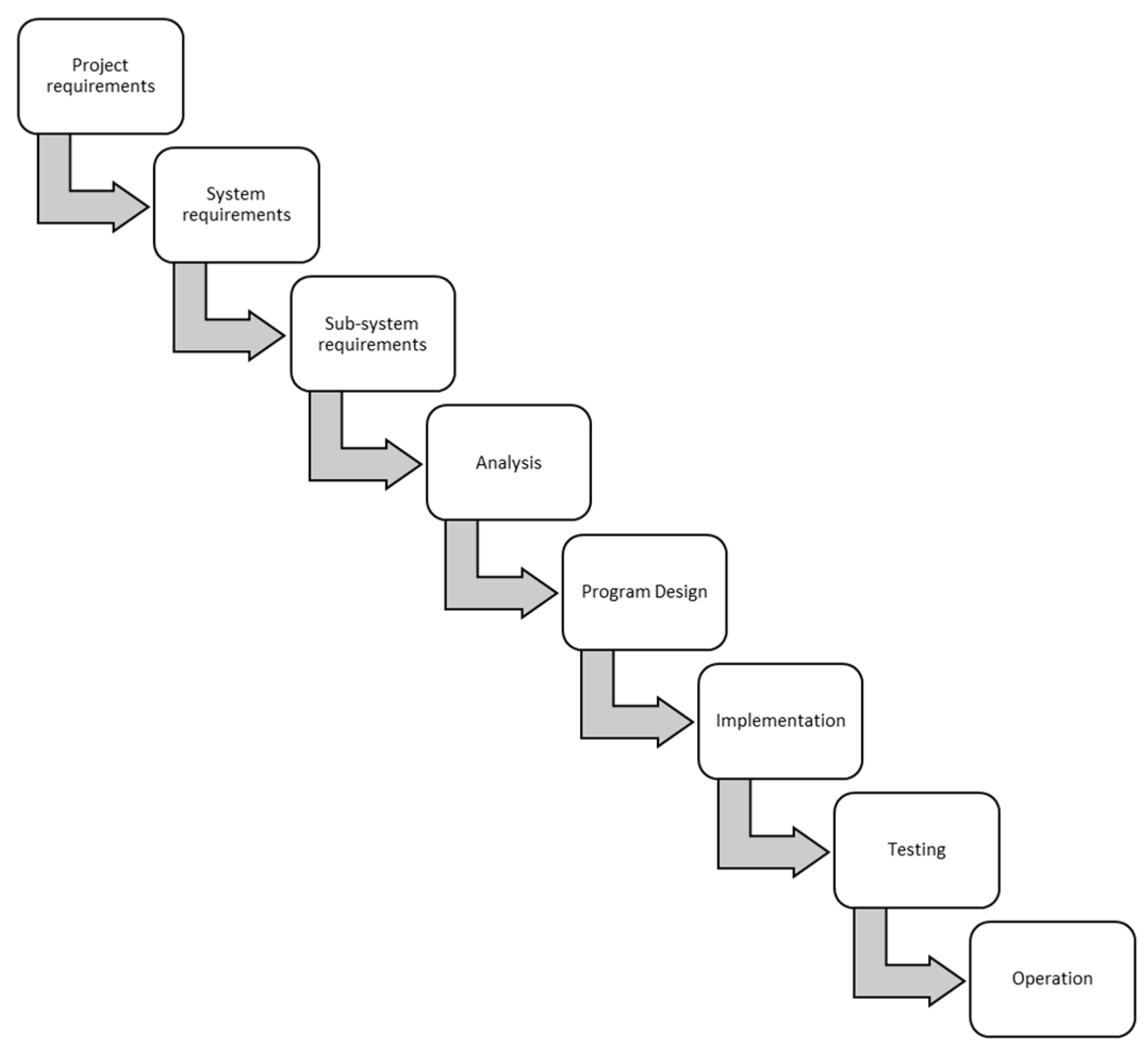
2.1.1. Traditional Approach

The conventional approach to product development, also referred to as the “Phase Gate Approach” or the “Waterfall” model, involves breaking down development activities into linear sequential phases, such as planning, designing, development, testing, deployment, and maintenance. Each phase is dependent on the deliverables of the previous phase and can commence only after the previous phase has concluded. Although in certain circumstances, it is feasible to step back to the previous phase, the model assumes that the process proceeds in one direction. The first known presentation describing the use of a Waterfall-like process for product development was given by Herbert D. Benington at the symposium on advanced programming methods for digital computers on 29 June 1956, where he outlined the development process of Semi-Automated Ground Environment (SAGE), a software developed for the US Air Force [14]. In 1970, Winston W. Royce presented his renowned phases process [15], which included a downstream drawing that bore a resemblance to the Waterfall as shown in Figure 1. Royce’s approach was adopted in 1985 by the United States Department of Defense as their standard [16], which encompassed six phases: “Preliminary Design, Detailed Design, Coding and Unit Testing, Integration and Testing”.

The Waterfall approach offers several advantages, including a clear understanding of project requirements before development begins and the ability to plan project resources and timelines in advance. This linear methodology is well-documented and easy to understand and implement, which explains its continued popularity. However, these advantages assume that there will be no changes to the project’s scope or requirements during the project lifecycle. The Waterfall approach lacks flexibility for such changes, requiring that all requirements be defined at the beginning of the planning phase. Any subsequent changes to requirements or design become increasingly expensive as the project progresses. Stakeholders only review results at the end of each phase or gate, after the work has already been done, meaning that introducing changes requires repeating certain tasks, which can impact other tasks and cause delays. This chain reaction of changes and rework can make it difficult to accurately estimate the duration, cost, and resources needed for the project, and the original project plan is often changed throughout the project lifecycle. As a result, the initial estimations can be misleading.

Over time, several modified versions of the Waterfall model have been proposed with minor or significant changes to overcome the issues identified in the traditional Waterfall approach. Examples of such modifications include the “Modified Waterfalls” proposed by McConnell in 1996 [17], and the “Sashimi Model” which involves an overlap between stages, as suggested by DeGrace and Stahl in 1990 [18], among others.

2.1.2. Iterative Approach

The “Spiral Model” is a development model that offers a unique perspective on the product development process. It was introduced in 1988 by Barry W. Boehm [19]. The model involves iterative development cycles where a prototype is created and evaluated by stakeholders. Subsequently, another development cycle is initiated to create a more detailed prototype with minimal effort to specify the overall product nature. With each development cycle, the risks are reduced until the prototype is robust enough and the risks are low enough. After this, the design continues similarly to the Waterfall model, with detailed design and testing. One significant advantage of the spiral model is the risk reduction and continuous feedback from stakeholders that occurs during the development cycle, rather than after, as is the case with traditional approaches. The “Spiral Model” iterative approach is very common today when using Agile methodology in NPD.

2.1.3. Lean and Agile Methodologies

The Lean approach was introduced as a solution to the typical issues with traditional approaches. Lean development is a translation of Lean manufacturing [20] to the Product development domain. The Lean philosophy is centered around streamlining workflow to create a product or service that customers perceive as having high value. The Lean approach prioritizes enhancing the value delivered to the customer while minimizing waste.

The publication of the Agile Manifesto in 2001 [2] sparked the emergence of new Agile methodologies that use iterative, interactive, and incremental development techniques and processes [21]. While there is no concrete proof that Agile methodology is founded on Lean philosophy, it appears that the latest Agile methods, such as Scrum, Crystal, Lean-Kanban, etc., which emerged in the early 2000s, are built around the idea of waste reduction and flow improvement, which aligns with a Lean-based approach. At present, the most widely adopted Agile methodology is Scrum [3,22]. Scrum is a conceptual framework based on short iterations, called Sprints [23]. Each sprint consists of the following stages: planning, developing, and reviewing. The development tasks are broken into small deliverables listed in a backlog; the backlog is arranged according to priority and is used as a bank of tasks for the upcoming sprint, being pulled when needed. During the sprint, changes are not accepted, but are welcomed between sprints. At the end of the sprint, the development team delivers a functional product that can then be evaluated by the customer or the product owner and, according to feedback, new tasks are created and added to the backlog for the next sprints. In addition, a retrospective meeting is held to look for ways to improve the process for future sprints. As the project advances, the product gains more and more functionality until the stakeholders are satisfied.

There are several advantages of using Agile-like techniques over the traditional ones; the biggest advantage is the flexibility of accepting changes during the development cycle, as the stakeholders get the chance to review the product while it is being developed and not receive it as a finished product at a late stage when the cost of changes are high. In reality, requirements are changing and as more information is gathered, there is a better understanding of what is needed, and requirements are added or eliminated. The Agile process increases the chances of delivering what the customer really needs [24] and not what it thought he needs before the project started. The main disadvantage of the Agile-like methodologies is the limited ability for future planning. Because the project is re-evaluated each sprint and requirements are being added or removed during the project life cycle, there is little use for planning ahead. As a concept and strategy, future planning in Lean or Agile is defined as a waste. The Agile methodology does not need and does not welcome long-range planning. However, managers and organizations still demand clarity and prediction of the future. The need for clarity is important for building the organization’s roadmap, allocating budgets and resources, planning company growth and more. This disadvantage is one of the biggest challenges in the adoption of the Agile methodology in organizations [24].

2.2. Choosing Strategy for NPD

All the models reviewed in this study are still in use in different variations; very few companies are using “pure” Waterfall (as presented by Royce) or “pure” Agile (as presented in the Agile Manifesto). Today it seems that each organization is developing products using its own hybrid methodology taken from the different models reviewed in this study and from the organization’s experience from past NPD projects. Each project and each product are unique. The projects are being affected differently from the methodology and actions applied to them; some strategies can work well with certain projects and can be complete failures with others. Each project requires a different approach to optimize its development process and there is no “one method that fits all” approach [1]. When selecting a development strategy, the system engineer and the project manager draws upon a combination of the company’s tools and standards, their personal experience, and common sense. However, currently, there are no practical and validated tools or techniques that compare various product development methods and management strategies. This makes it difficult to understand the impact of each strategy on a specific project.

A project life cycle is not linear, as it may be presented in some models, and people are making decisions based on the state of the project. These decisions cause other changes and lead to a new state upon which they make new decisions. This chaos reaction of project changes [25] limits the ability to predict the effect of a single change on the entire project and makes it nearly impossible to predict the effects of multiple changes as they happen in real life [26]. For example, a delay in completing a task may cause further delay in starting other tasks that depend on it. If the deadline of the milestone is near, the work rate and the decisions that will be taken will not necessarily be the same if the milestone deadline is far away. The “schedule pressure” effect [27] is one example of an effect that does not appear in standard scheduling models and can have a significant effect on the project’s schedule.

2.3. Project Success

The main reason for project failure, as indicated by the PwC survey [28] and the Chaos report [29], is “Poor estimates/Missed deadlines”. In another study [22], managers from leading organizations identified “Project Scheduling” (83%) and “Product Quality” (57%) as their top criteria for project success, with other criteria, such as “Project Cost”, ranking lower. However, despite project scheduling being considered the top criterion for project success, project delays are still widespread. Many projects fail to meet their deadlines, with only 30% of projects delivered on time according to KPMG [30], and only 40% delivered on time according to The Standish Group database from 2011 to 2015 [29]. Similar findings have been reported in other studies [22]. Given these findings, it is evident that product development methodologies are crucial, and there is a need to improve project scheduling planning and prediction. Therefore, this research aims to enhance the planning and estimation of project scheduling.

2.4. Simulation Modeling of New Product Development Projects

2.4.1. Simulation Model

A Simulation model is a research methodology that involves conducting dynamic experiments to comprehend and predict the behavior of a system within certain limitations [31]. This approach enables simulation models to be employed for a range of purposes such as planning, control management, process improvement, training, and learning [32]. In product development, simulation models have been used to explore several areas including requirements management [33], product reliability [34], and product testing [35]. Modeling and simulation are critical components of the new product development process, they are used to test a design before production, and are mandatory part of NPD standards [36].

2.4.2. System Dynamics Modeling

Jay W. Forrester from the Massachusetts Institute of Technology developed the system dynamics approach to modeling in 1961 [37]. This methodology integrates theory, philosophy, and techniques to model and analyze complex systems with feedback loops. It characterizes the dynamic behavior of nonlinear and complex systems that include dynamic variables that change over time. The approach describes the system’s behavior by its element structure in a closed loop, creating the feedback loop responsible for changes over time. The feedback loop shows that activity A influences activity B, which in turn affects activity A and so on. It is crucial to comprehend the relationship between A and B separately, as well as the connection between B and A, which may differ. Observing the entire system’s behavior is also critical to model its outcomes. The system dynamics model is a mathematical model that employs a set of differential equations to describe the system. Creating these equations involves a qualitative stage of modeling a causal loop diagram (CLD). The CLD demonstrate the chain effects of a dynamic process where the causes are traced through a set of interconnected variables and back to the original cause. The CLD represents both positive and negative correlations between the connected variables or factors, aiding in their conversion into a quantitative structure diagram. The variables in the structure diagram are categorized into Levels and Rates (or Stocks and Flows), auxiliary variables, and constants. Levels indicate the quantity of an element, such as the amount of water in a tank, the number of resources available for the project, and so on. Rates represent the rate of change of the Level over time (increasing or decreasing); the Rate variable is directly linked to the Levels, determining their rate of change value.

Solving the equations that reflect the behavior of a system can be challenging, particularly if random variables are involved. Thus, simulation is crucial to properly analyze a system dynamics model. Standard simulation runs can be used to model deterministic scenarios. However, for comprehensive analysis of the entire system behavior, tools like Monte Carlo simulation [38] can be utilized to model the probability of various outcomes.

2.4.3. System Dynamics in Project Management

System Dynamics has been widely utilized in various research projects and studies. Its first practical application in project management modeling was carried out by Pugh-Roberts Associates to support a significant claim made by Ingalls Shipbuilding against the US Navy in the 1970s. Kenneth G. Cooper developed a model that described the causes of cost and schedule overruns on a multibillion-dollar shipbuilding program, resulting in a $447 million-dollar settlement for Ingalls Shipbuilding. One of the key innovations of Cooper’s work was the modeling of the rework cycle in a project [39]. This model described the concept of undiscovered rework, which is prevalent in NPD projects, and included variables such as the time to discover rework, work quality, and varying staff productivity.

Many project management models have utilized the concepts developed by Cooper, including a model by Richardson and Pugh [40], which describes the basic feedback structures of the project management process and demonstrates the trade-off between meeting the schedule and acquiring additional resources. The Program Management Modelling System (PMMS), which was developed by Pugh-Roberts Associates based on Cooper’s work, is one of the most extensive models to date and is being employed to manage large programs. While the PMMS is conceptually described in Lyneis [41] and Pugh-Roberts, the model itself is not available for evaluation or comparison.

According to Lyneis & Ford [42], project management has been the most extensively and successfully used application of system dynamics. Pugh-Roberts Associates have applied system dynamics modeling alone in over 30 contract disputes. There are also system dynamics models that address issues in human resource management and planning and control of software projects [43]. Williams et al. [44,45] have used the system dynamics model to identify feedback processes responsible for the effect of work being developed in parallel, which can lead to longer activity durations and increased parallelism that may cause the project to struggle in meeting its original deadlines. Ford and Sterman [46] presented a detailed model of a multiple-phase project that includes the project process, resources, and scope, based on past studies using objects from the PMMS model. In addition, Taylor and Ford [47] used rework and ripple effects to model the tipping point structure in development projects based on the Ford & Sterman model.

3. Research Description

3.1. Research Goal

The main goal of this study is to develop a systems dynamic model to study of the impact of the product development methodology on NPD projects timeline. This was done by development of an NPD project model which covers Waterfall, Spiral, Agile and Hybrid product development methodologies. The model is used to simulate the effect of each type of methodology on the project results. In order to validate the model and to demonstrate its consistency with reality, we used real projects use cases from different organizations.

Another goal of this research is to test the use of the proposed model and simulation as a tool for system engineers and project managers. The model can be used as a utility tool which supports system engineers and project managers’ decisions and helps them to decide on the project strategy that best suits their project. The model allows good estimation of the project deadlines and can help managers to better plan a project and to make better management decisions. The tool is not limited to a pure Agile nor pure Waterfall methodology; it allows one to take processes and techniques from one methodology and integrate them with processes and techniques from other methodologies, creating a hybrid method which best fits the specific project. The proposed model supports a better understanding of the properties which make a project more suitable to a certain strategy than to another and to develop rules which can increase the probability for project’s success.

3.2. Significance of the Study

The research results provide a new set of tools for system engineers and project managers. The tools were validated and tested on real projects. Validation with real projects differentiates this study from many other studies and models which had been developed and stayed on the theoretic stage. The tools are not limited to a certain project management methodology and can be used side-by-side with any other tool in order to allow more effective and better management decisions. The model will be able to improve NPD projects’ duration estimation, identify the processes which contribute to achieve the project goals, as well as the ones that are risky for the project.

We believe that this study can have ancillary objectives beyond the scope of the research questions and can benefit researchers interested in an in-depth study of product development methodologies such as Agile and Waterfall. The research results can provide a basis for further research. A validated model proven to be consistent with reality could be used for testing researcher’s hypotheses, reviewing new and old development methodologies, allowing a further extension to fit other types of projects and more.

To the best of our knowledge, with respect to the literature, there is no prior work on a validated NPD model that tests the application of different development methodologies on a project to understand the expected effect of each methodology on the project duration.

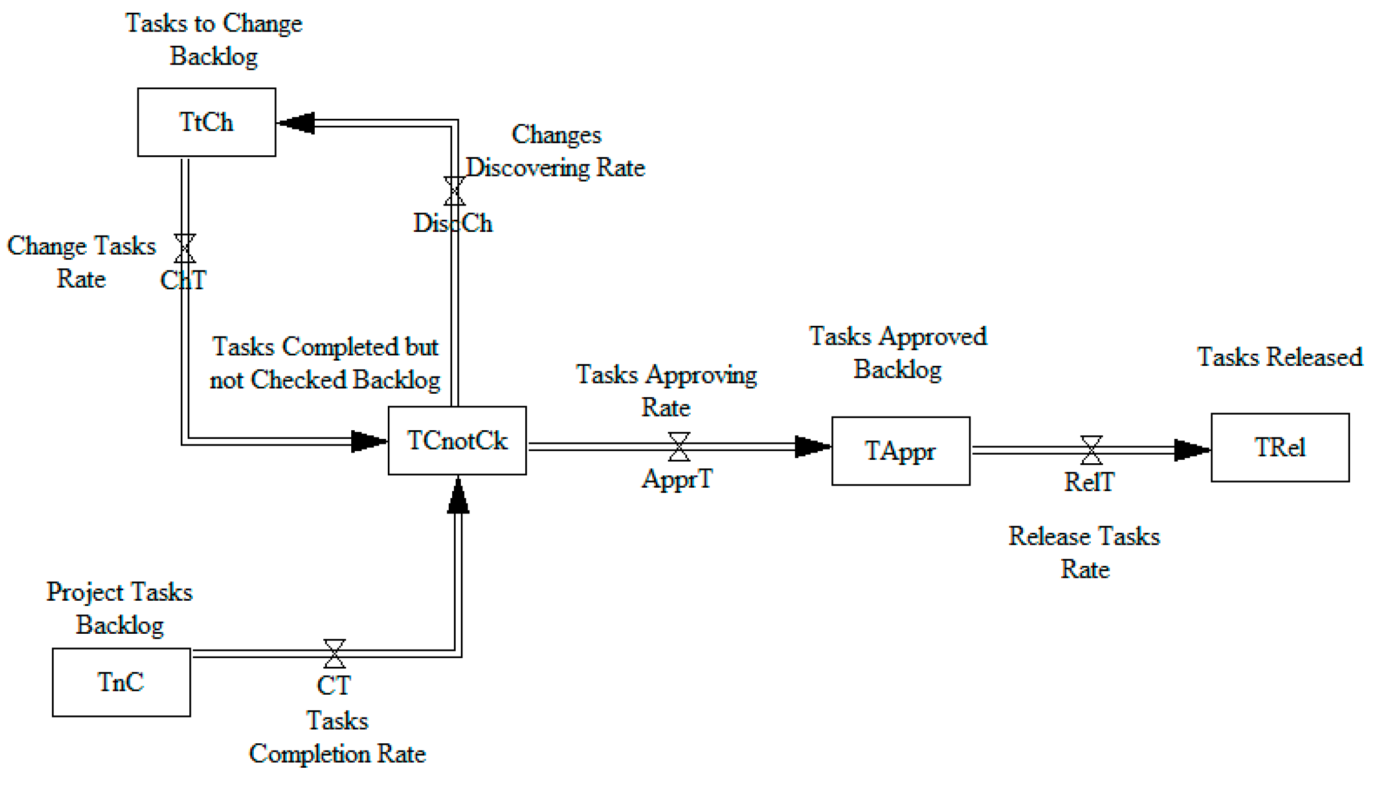
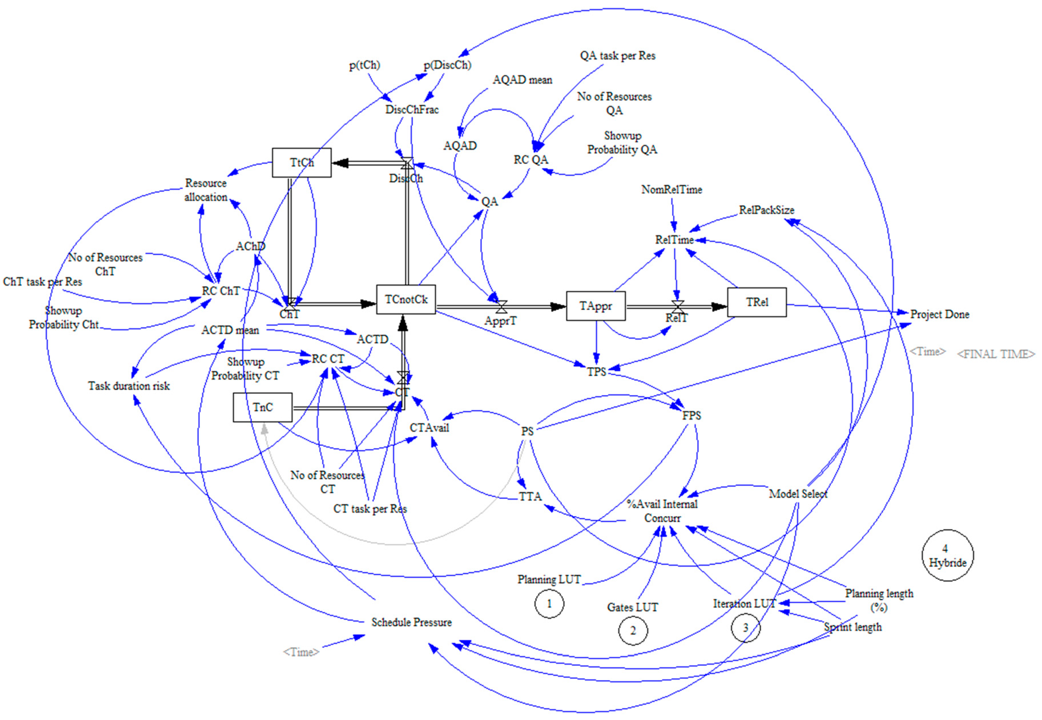
4. Model Description

The proposed NPD model was developed using the Vensim PLE system dynamics modeling tool. The model core is built upon the published model of David N. Ford and John D. Sterman [46] with an additional view of NPD project management studies in which characteristics of NPD projects from different methodologies have been examined. Ford and Sterman based their model on Pugh-Roberts’ well-known models and utilized objects from the PMMS model. Their model’s core is centered on the “Rework Cycle” paradigm, which was first published by Cooper [39]. This paradigm identifies undiscovered errors in the current work, which leads to more work in correcting these errors. As more work is done, more errors are produced, leading to a recursive nature of the project where rework generates more rework, resulting in the creation of more tasks that need to be done to complete the project or a phase of the project. The proposed NPD model’s foundation is shown in Figure 2, which includes four task backlogs in the project pipeline: “Project Tasks Backlog”, “Tasks Completed but not Checked Backlog”, “Tasks to Change Backlog”, and “Tasks Approved Backlog.” The tasks flow from one backlog to another according to the Rates presented in Figure 2. The resource allocated to these tasks limits each of these Rates.

The following improvements were implemented to the basic model presented in Figure 3 which is based on the Ford and Sterman model:

4.1. Stochastic Variables Instead of Deterministic Variables

The original model uses deterministic variables for setting the rate of task execution, for example: “Average Completion Duration” and “Resource Constraint”. In the proposed NPD model, more variables were added, such as: “No. of Resources”, “Resource Show-Up Probability”, “Task Mean Duration” and more. In addition, the deterministic variables such as “Average Task Duration” and more were replaced with stochastic variables according to a distribution function allowing one to control the mean and the std. deviation of the function. Moreover, the “Resource Constraint” is now relying on the “Resource Allocation” and “Show-Up Probability”, which is a random variable that represents the probability of a resource being available to perform the tasks, since not all resource types can have an assured 100% availability rate during the project life cycle.

4.2. Risk Management

Any NPD project has risks associated with it. There is a probability of risk events happening that may affect the duration of some of the project’s tasks and cause a delay in the project’s scheduling. The proposed NPD model includes a function of “Task Duration Risks” which contains the average probability that tasks have of taking longer due to the expected risk; this probability is being considered with each task duration calculation. The Risk function impacts the duration of tasks, utilizing a Normal distribution with a standard deviation determined by the project risk assessment. For each task associated with risks, the probability of an extension in its duration is calculated. This probability is also linked to the project’s progress and the number of tasks completed successfully. This is based on the assumption that as the project progresses, risks are typically reduced until the project concludes and all risks are eliminated.

4.3. Dynamic Allocation of Resources

In the original model, the allocation of resources is fixed, meaning that if a resource is not being used due to lack of tasks in the backlog, the resource is not exploited by other tasks as may happen in reality. In the proposed NPD model, the option for automatic resource allocation was added and it can be configured according to the project definition. For example, if the “Tasks to Change Backlog” is empty, meaning there are no tasks to change, the resources which were allocated to that task’s backlog can be reallocated to help complete tasks from another backlog, such as the “Project Tasks Backlog”. The model allows one to choose the automatic allocation rules.

4.4. Gates (Waterfall) Mode

In order to model the project lifecycle in Gates mode (Waterfall), one needs to load a lookup table of the Gates available in the project and the tasks need in order to pass the gate; the Gates LUT loads this information from an excel file and creates the gates in the model by allowing working only on the tasks available before approving the next gate. Gate can be approved when all of the tasks related to the gate are completed, tested, and approved by the testing team.

4.5. Iterations (Agile/Spiral) Mode

In order to model iterations methodology which is aligned with Agile and Spiral methodology, we based it on previous studies of modelling Agile methodology [27,48,49]. The Iterations mode uses the parameters of Sprint Length in order to set the length of each sprint; the overhead of sprint planning is set by Planning Length parameter and another factor that is dominant in Iteration mode is the Schedule Pressure [27] that dynamically changes the average productivity of the team (ACTD_mean) as the end of the iteration is coming, but also affects the quality of the performed tasks and the probability of finding errors (P(DiscCh)).

4.6. Hybrid Mode

As many organizations do not use pure Agile or pure Waterfall, the need to model a hybrid mode is clear. The hybrid mode keeps the options of Gates while allowing work on short/long iterations between Gates. The type of gates, the length, and the scope of the iterations together with all other parameters that are relevant for both Gates and Iterations mode are available in order to adjust the model to fit the unique Hybrid mode of each project and organization.

4.7. Model Verification

As the proposed model is based on a well-known well validated model [46], the verification process primarily focused on the introduced modifications. The model verification process encompassed the following:

• Ensuring Unit Consistency: Verification involved confirming that units remained consistent across the entire model. This included checking units for all parameters, variables, and equations.
• Verifying Boundary Conditions: This step ensured that the model incorporated suitable boundary conditions, and that the system’s behaviour was well-defined within those boundaries.
• Conducting Sensitivity Analysis: Sensitivity analysis was performed to evaluate how the model responded to changes in parameters. This facilitated the identification of critical parameters and assessed the overall robustness of the model.
• Checking Initial Conditions: Verification confirmed that the initial conditions of the model were appropriate and realistic for the system under consideration.
• Verifying Equations: The mathematical equations used in the model underwent a thorough review and verification process. This included checking for accuracy in representing the dynamic relationships among variables.

Appendix A provides a comprehensive presentation of all parameters and equations utilized in the proposed NPD model.

5. Results

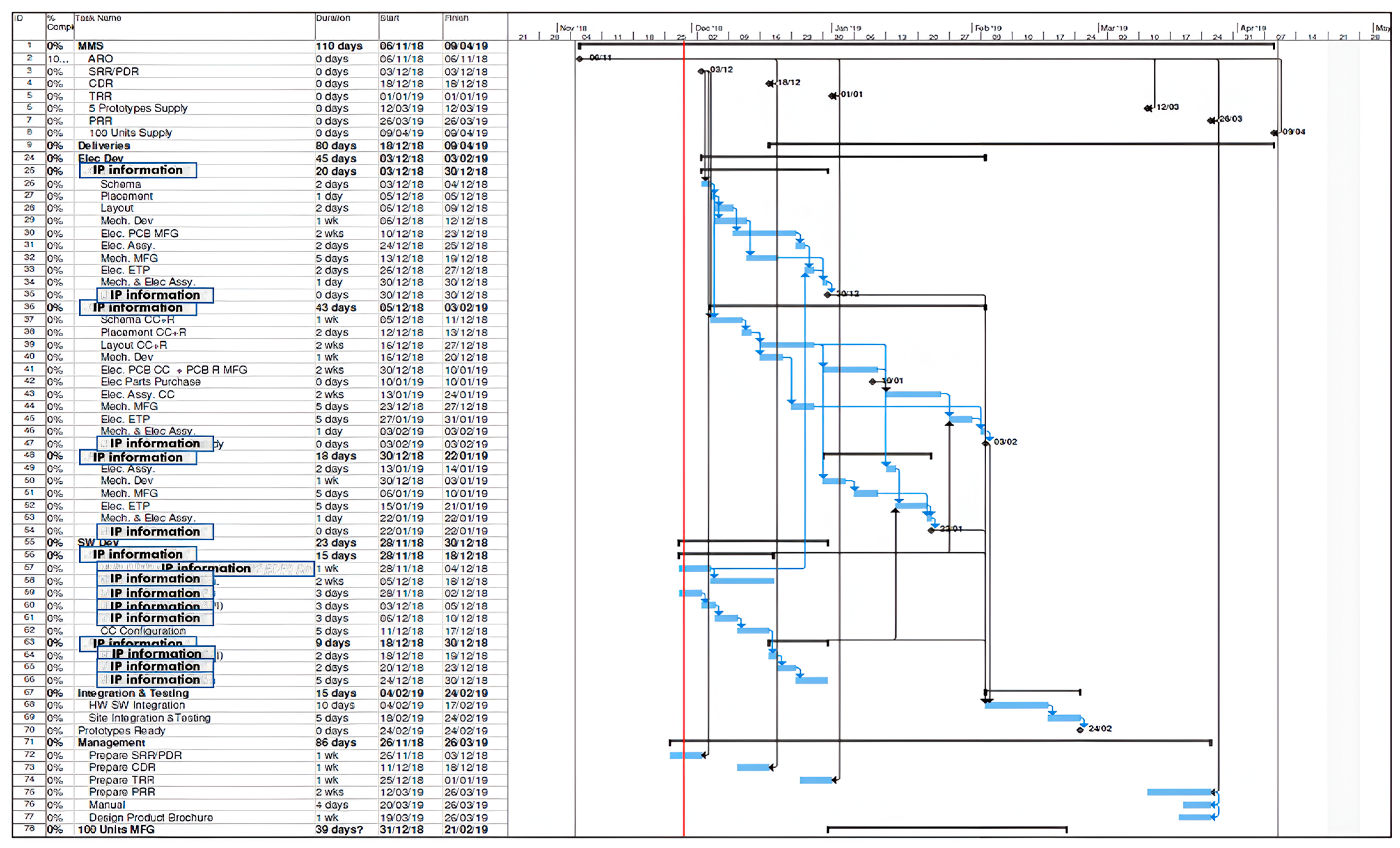
5.1. Waterfall (Gates)

5.1.1. Waterfall Model Validation

The presented NPD model core is based on a well validated model of David N. Ford and John D. Sterman [46], with the improvement of adding stochastic parameters instead of deterministic. To validate the Waterfall mode of our proposed NPD model, we drew upon data from a 2019 development project involving a multidisciplinary IoT (Internet of Things) system. This project encompassed Mechanical development, Electronics development, and Software development. The data extracted from this project comprised the initial Gantt chart, resource details, project management methodology specifics, and information regarding project risks. The project adhered to the Waterfall project management methodology. The initial Gantt chart for the project included 38 development tasks with an average duration of 4.55263 days per task and with expected 15 days for product testing, meaning an average of 0.39474 days per task. Four engineers were allocated for the project; the engineers were in charge of the development, QA tests, and correction cycles. The resource allocation was estimated as follows: 50% for development, 25% for testing, and 25% for correction cycles. According to the initial Gantt of the project, the estimated duration for the entire project was 110 working days. Appendix B presents the initial Gantt chart of the IoT project.

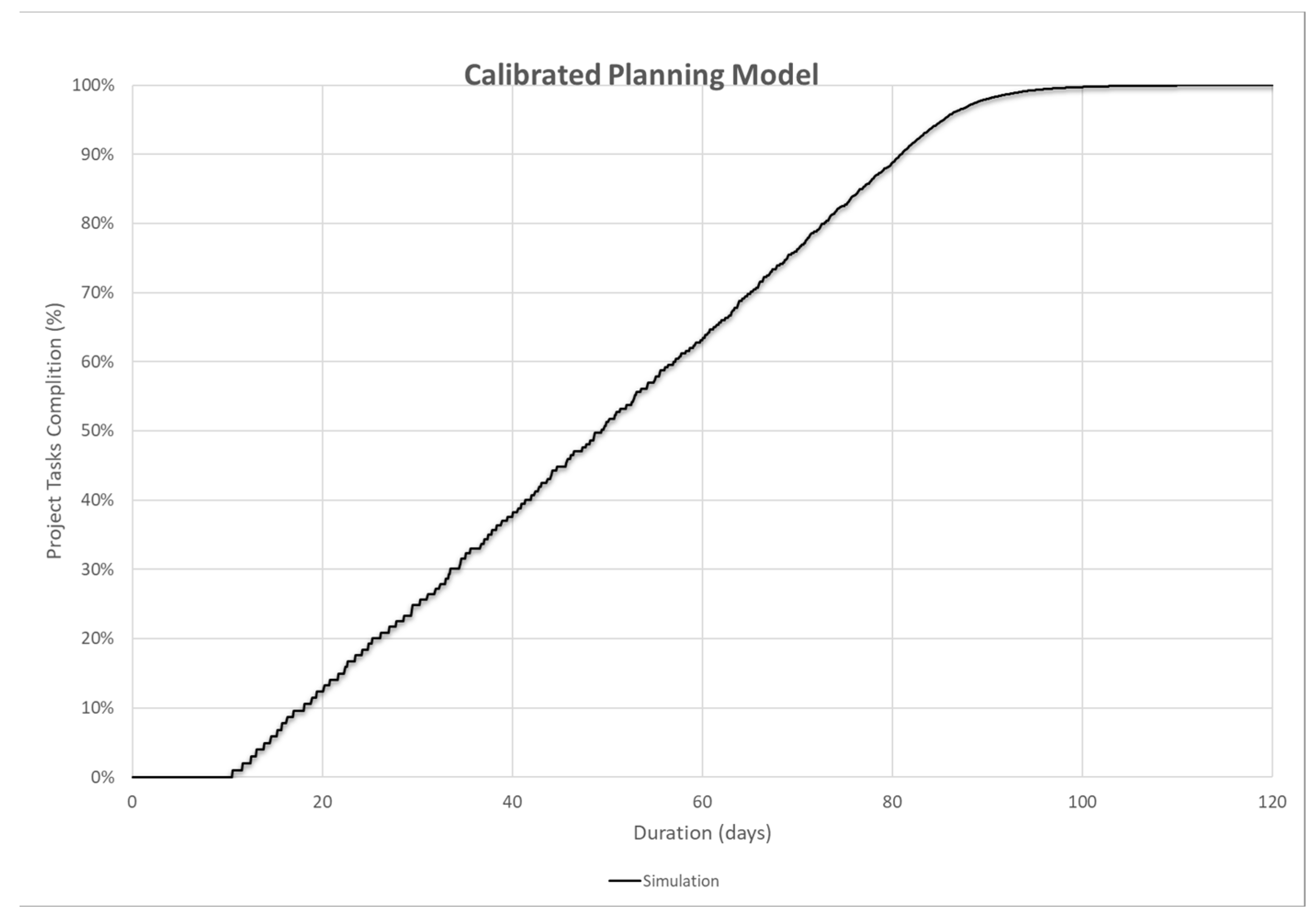
5.1.2. Calibrating the Model

The model calibration process involves inputting project information into the model, which includes the following parameters: Number of Tasks, Average task duration, Average testing duration per task, Resource information, Estimation of the probability of a task requiring a change, and Probability to discover a change. Once the information is entered, a data validation step is performed by running the model in “Planning Mode.” This mode replicates the project “as is” without any additional features or properties. The expected outcome is that the simulation duration will closely resemble the estimated duration provided by the Gantt chart which in this case is 110 days. After trimming the model parameters, the calibration results are shown in Figure 4 which illustrates the estimation for completing 100% of the tasks according to the planning model, in consist to axis the duration of the simulation and the amount of project tasks completed at each time. The linearity of the graph is the indication that the project plan is reflecting “ideal mode” which there is always a progress in the project tasks and no delay, which hardly happens in reality.

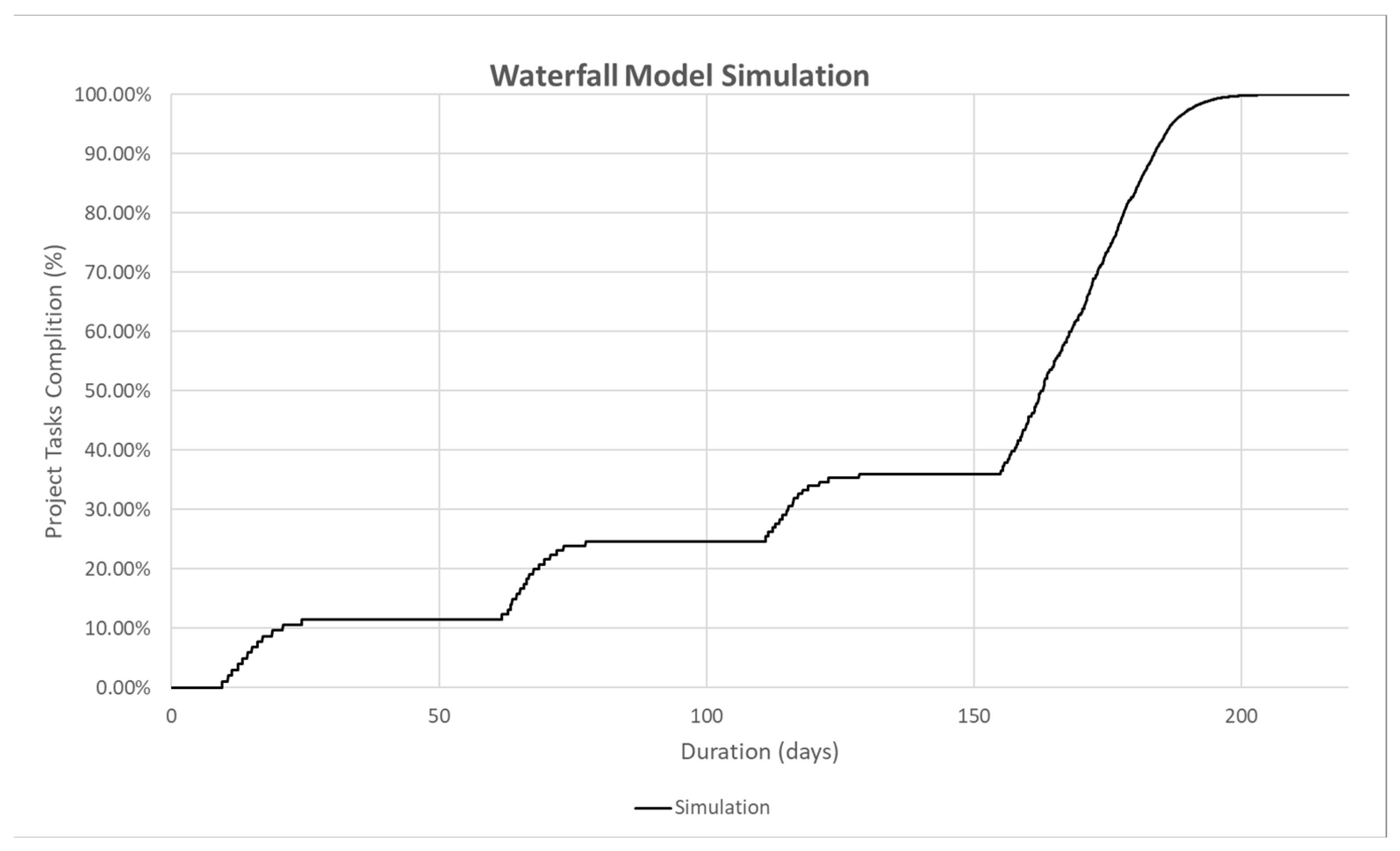
5.1.3. Simulation of the Project Life Cycle

In order to apply a simulation of the project’s life cycle, the methodology type needs to be set to a Waterfall by choosing the “Gates” approach. According to the project Gantt, there are 4 phases (or gates) to the project: PDR, CDR, TRR and PRR. To pass a gate, certain tasks have to be completed; if the tasks are not complete the gate will not be approved, and the project cannot continue. According to the project’s Gantt chart: PDR will be held when 20% of the project is completed, CDR will hold on 31%, TRR on 42%, and PRR when the project is almost completed. As organizations may exhibit diverse behaviors, the selection of the distribution function for each stochastic parameter can be determined through measurements or by consulting various studies in the field [50,51,52]. In this particular case study, we incorporated the following information based on the organization’s data: Resource Show-up probability—modelling the probability of resource availability to work on a task. In this case we set the parameter to 0.95, meaning that the resource availability has Normal distribution with a mean value of 95%.

• Task duration distribution—modelling the probability of a task taking longer or shorter than planned.

The simulation results of the project Waterfall simulation are presented in Figure 5. As observed, the progress in the Gates mode is non-linear, slowing down as the project approaches a gate and coming to a halt upon reaching it. This occurs due to correction cycles required for gate approval and numerous tasks that cannot be executed until the gate is approved. In this scenario, the model estimates 204 working days for completing 100% of the project.

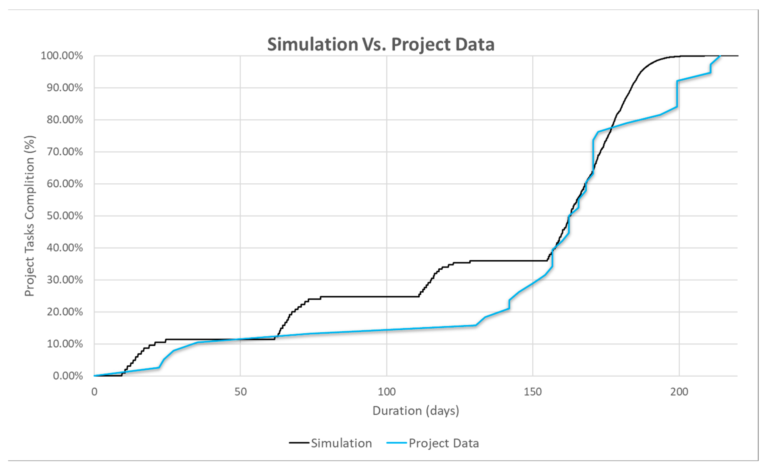
5.1.4. Comparing the Simulation to the Project Results

The results of the project were taken from the last updated project Gantt chart of the project which reflected the status of the project at its end. The graph in Figure 6 shows both the simulation results and the real data on the same graph. As can be seen in Figure 6, the Gates curve demonstrated in the simulation is also reflected in the real data. Although the timing of the gate is not aligned throughout the entire project, there is noticeable alignment at the beginning and end. The reasons for this misalignment will be further discussed in the paper. The maximum differences between simulation and true data during the project life cycle was on the 130th day when the simulator estimated that ~36% of project’s tasks were completed while according to the project Gantt chart, only 15.79% of the tasks had been completed—which means a differential of ~16%. When comparing the end time of the project, the project’s actual duration was 214 working days while the simulation’s prediction was 204 working days which resulted in a prediction with an accuracy of 95%.

5.2. Agile (Iterations)

5.2.1. Agile Model Validation

The Iteration mode is based on well study models [27,48,49] that have been integrated into the primary project management model that is presented in Section 5.2. In order to test the Iteration component of the model, we utilized data from an ongoing 6-month project conducted by a startup company, spanning from October 2022 to March 2023. The project encompassed the development of a mobile application, cloud-based backend services, and a web-based application. The sprint length was set as 2 weeks, with 1 day allocated for retrospective and sprint planning activities between the sprints. Task management was facilitated using a Kanban board system. At the project’s outset, three main epics were identified: Mobile application, Cloud services, and Management web application. After each sprint, product releases were made, and the subsequent sprint tasks were determined based on feedback from stakeholders and customers. Throughout the project, a total of 13 sprints were conducted, each sprint lasting two weeks (10 working days), resulting in a total of 125 working days (after accounting for holidays). Each task was documented using a Kanban ticket, with tasks durations ranging from 1 h to 2 days, and an average task duration of 0.8 days. The development team consisted of 6 resources: 4 software developers, 1 QA specialist, and a team leader who served as the scrum master and product owner. A total of 516 tickets were opened during the project, but only 456 tickets were executed.

5.2.2. Calibrating the Model

The model calibration process involves inputting various project information into the model, such as the Number of Tasks, Average task duration, Average testing duration per task, Resource information, Estimation of the probability of a task requiring a change, and Probability to discover a change.

In addition to the aforementioned parameters, certain adjustments were made for calibrating according to the unique properties of organizations. The Resource show-up probability was set to follow a normal distribution with a mean value of 0.9. The probability of discovering changes in tasks was connected to the Schedule Pressure variable, which can reduce the probability by 50% on the last day of the sprint. The sprint length is directly related to the probability of rework, as shorter sprint will require less rework due to the agility of feedbacks. On this case the sprint was set to 10 days, so a 10% probability was set for changing tasks that have already been implemented. The number of tasks was specifically set to 456, corresponding to the number of tasks identified in the project case study.

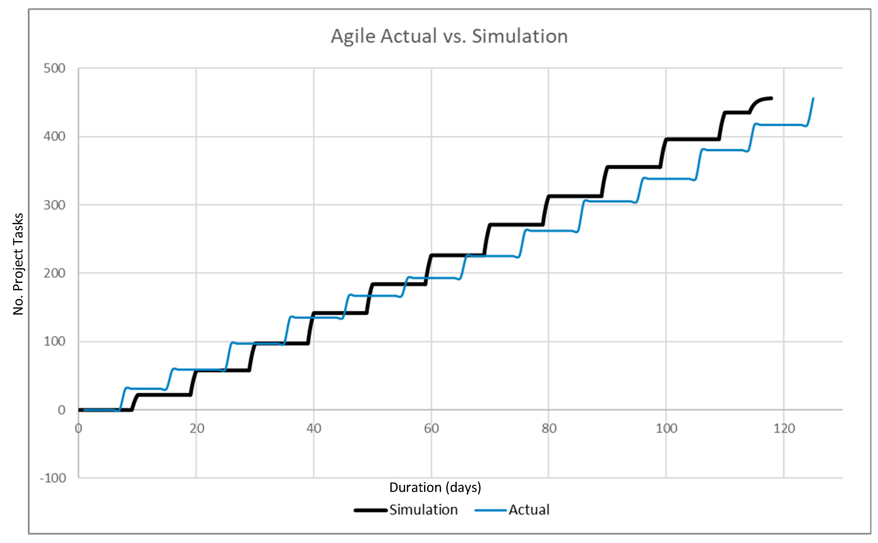
5.2.3. Comparing Simulation to the Project Results

By entering this information into the model. The simulation finished the 456 tasks between 12 sprints and a duration of 117.9 days, while the actual project data indicated 13 sprints with 125 working days (after reducing holidays). To calculate, the prediction of the project duration gives a differential of 7 days which translated to accuracy of 94%. Figure 7 illustrates the actual versus simulation graph. In this graph, the work is organized in sprints, and the release of work occurs solely at the end of each sprint. The absence of ongoing releases results in a “steps” diagram, with progress being measured exclusively at the conclusion of each sprint.

5.3. Choosing a Different NPD Strategy

As a case study we took the IOT project presented in Section 5.1. As mentioned, the project used Waterfall methodology, the resources include 4 engineers, 38 tasks with average duration of 4.55263 days per task. The Waterfall simulation estimated the project duration as 204 working days. Our aim is to understand how adding additional resources will affect this project’s duration. We added additional resource (total of 5 engineers) to the team and ran the simulation again. The results in

Table 1. Simulation results of strategic changes in the tested IoT Project.

Strategic Change	Project Duration	Difference from Original
Additional resource unit	188	−16 (7.8%)
Additional two resource units	182	−22 (10.8%)
Agile methodology	153	−51(25%)

showed that the duration estimation decreases from 204 working days to 188, total of 16 working days that translated to 7.8% shorter timeline, while the incrementation in resource was 25%. In projects where the timeline is more important than cost, the project manager can consider adding another resource. When adding another engineer (total of 6 engineers), the duration decreases in another 6 days (3.2%). As can be seen, there is no linear correlation between the number of resources and the duration of the project. The core reason is mainly because there is precedence relation between tasks and parallel work is limited.

Another strategic decision a project manager can use the simulation for, is choosing different development methodology, such as Agile. We set the Methodology to Iteration, with sprint length of 10 working days, no change with resource allocation and quantities. The simulation shows that the project will end after 153 working days. This means a reduction of 25% in working days without changing any resource level. The reduction in timeline was made mostly due to the fact the less rework needed to be done and the team continued to develop and didn’t stop at the Waterfall gates. Choosing the right length of the sprint is also an important factor in Agile-like methodologies. Using the proposed simulation, we chose different possible sprint lengths and measured the effect on the project duration. The results in

Table 2. Sprint Length effect on the tested IoT Project.

Sprint Length	Project Duration	Difference from Previous
1 weeks	149	-
2 weeks	153	+4
3 weeks	161	+8
4 weeks	170	+9
5 weeks	175	+5
6 weeks	199	+24
7 weeks	209	+10

presents that on this project shorter sprints results in shorter project duration, as this project probably needs this agility. Thus, the differences between 1 and 2 weeks sprint are not very significate (4 days difference). In 6 weeks and above the agility of the iteration is not good enough, so if long sprints are required, Waterfall will bring shorter project duration.

Thus, since we do not have enough information about this project or whether a pure Agile could be implemented, we also tested one type of Hybrid use case. We set the simulation methodology as Hybrid, which allowed keeping the same gates constrains as in the original project and added the ability to work in sprints for part of the tasks, this allowed the reduction of the amount of pre-planning duration, but kept some of the Waterfall processes. The chosen hybrid methodology simulation results estimated the project will end after 167 days (18.1% working day reduction from the original Waterfall simulation).

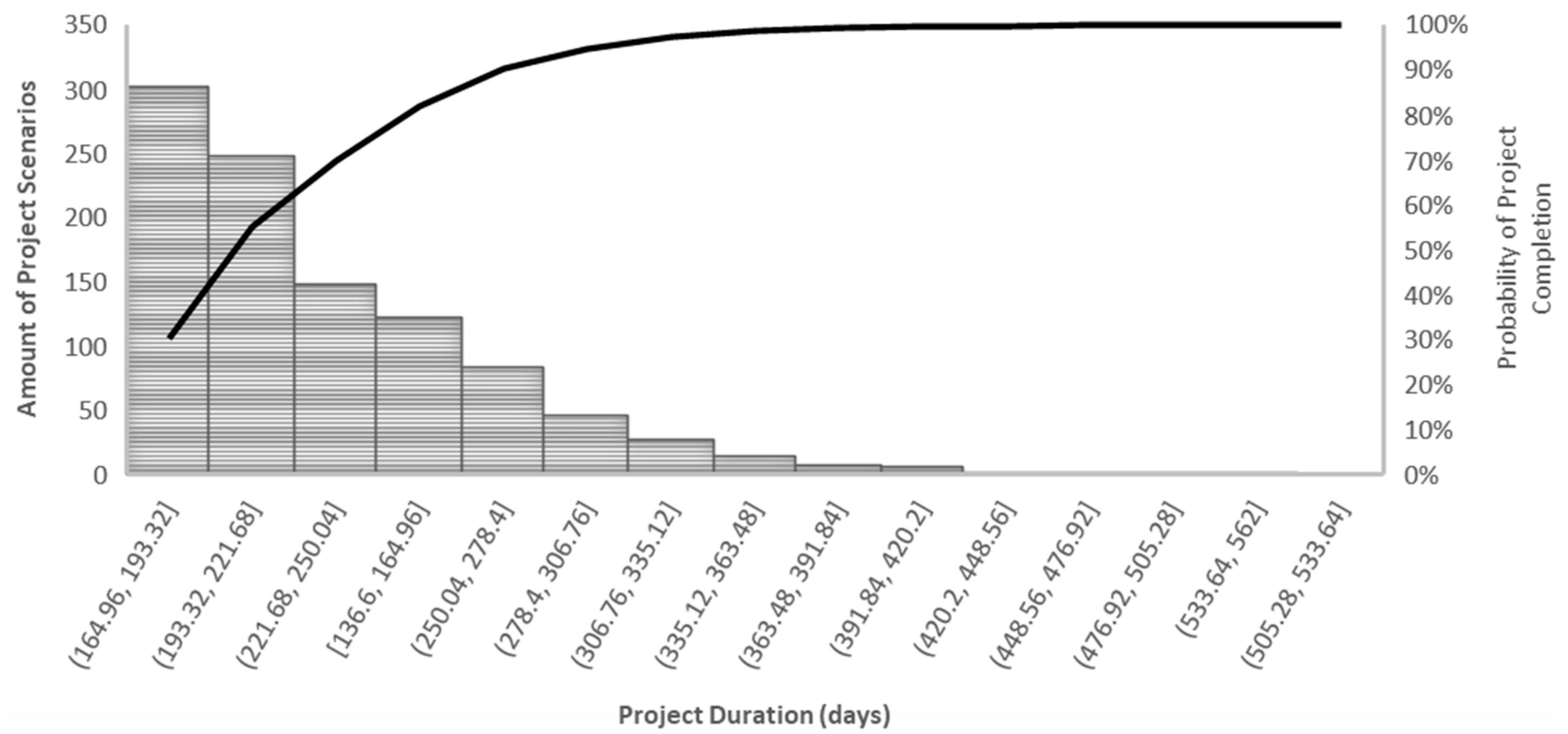
5.4. Sensitivity and Monte Carlo Analysis

Risk analysis is a widely employed technique in project management to evaluate the likelihood of changes that may impact project deadlines. Implementing risk mitigation strategies can reduce the probability or impact of these risks. However, the decision to apply these mitigations is often complicated by the associated costs. To gain a comprehensive understanding of the effects of risk reduction, sensitivity analysis can be conducted using simulation methods. In this study, we performed a risk analysis on the project by varying the value of p(tCh) in the model, which represents the probability of changes occurring in the project. A change or disruption in a project is defined as work performed out of sequence, while an excessive number of disruptions and changes can trigger a “ripple effect” that exponentially increases the project’s duration compared to a linear increase in disruptions [53]. To conduct the simulation, we held all project parameters at fixed values and solely manipulated p(tCh). In addition, we conducted the same analysis on the project in an Agile methodology mode and compared the results. This comparative analysis provides insights into the performance of different development methodologies in the face of changing probabilities of the project to experience changes. The outcomes of this analysis, as presented in

Table 3. Waterfall vs. Agile Sensitivity Analysis on the tested IoT Project.

p(tCh)	Project Duration (Waterfall)	Project Duration (Agile)	Difference
0%	121	159	−38 (−31%)
5%	136	159	−23 (−17%)
10%	143	159	−16 (−11%)
15%	150	160	−10 (−7%)
20%	156	160	−4 (−3%)
30%	173	169	4 (2%)
40%	193	189	4 (2%)
50%	222	216	6 (3%)
60%	255	250	5 (2%)
70%	308	289	19 (6%)
80%	374	359	15 (4%)
90%	487	443	44 (9%)

, demonstrate that for this particular project, the Waterfall methodology is preferred in terms of project duration when the probability of changes remains up to 20%. However, beyond a 20% probability, the two methodologies exhibit similar performance, with a slight advantage towards Agile. Notably, the Agile methodology starts to exhibit significantly shorter durations when the probability of changes exceeds 70%.

This case study contributes valuable information for decision-making regarding the selection of the most suitable development methodology and the need for risk reduction. System engineers, project managers and other stakeholders can leverage these findings to determine the appropriate approach for managing risks and optimizing project duration based on the specific context and probability of changes.

The trial-and-error approach is a valuable method for testing specific scenarios in project management. However, to achieve scalability and explore a broader range of possibilities, the implementation of Monte Carlo analysis offers a more efficient approach. This analytical technique enables the execution of numerous project scenarios, encompassing diverse combinations of parameters, thereby providing a comprehensive overview of various strategies and their impacts on project duration. Subsequently, the project manager can carefully select a strategy that appears suitable and proceed to conduct a more concise Monte Carlo analysis by fixing the base parameters with predetermined values. An essential aspect of the proposed model is its incorporation of stochastic parameters. Running the project simulation multiple times generates a histogram that effectively illustrates the distribution of project durations. This histogram serves as a valuable tool for the project manager to assess the robustness of the project plan and strategy while also determining the probability of the project lasting a specific duration. By analyzing the histogram, it becomes possible to calculate and comprehend the probability of successfully completing the project within the desired time frame using a particular strategy. Additionally, the comparison of histograms derived from different strategy approaches enables the project manager to select the approach that aligns best with the project’s success criteria. To demonstrate the effectiveness of Monte Carlo analysis, Figure 8 presents the results of a project case study. In this analysis, the project simulation was executed 1000 times using the project’s original parameters. The actual duration of the project was measured as 214 days, and according to the simulation results, there was approximately a 60% probability that the project would be completed within 214 days, with a remaining 40% probability of exceeding that duration.

The application of Monte Carlo analysis, coupled with the interpretation of the resulting histogram, provides valuable insights into the distribution of project durations and the associated probabilities of meeting specific deadlines. This approach empowers project managers to make informed decisions by offering quantitative data that supports the selection of effective strategies and enables a comprehensive evaluation of project success probabilities. By leveraging the benefits of Monte Carlo analysis, project managers can enhance their understanding of project dynamics, optimize resource allocation, and improve overall project performance.

6. Discussion and Conclusions

The selection of an appropriate methodology for a specific project holds significant importance and should be made during the early stages of project planning. This decision directly influences various aspects of the project, including resource allocation, budgeting, expected outcomes, and scheduling. Current methods for choosing new product development project strategies largely rely on organizational culture and team experience. However, in this paper, we have presented a simulation model that is based on a validated system dynamics model of the project life cycle. This model allows users to input project parameters, calibrate the model accordingly, and test different project strategies.

The simulation model we presented focuses on the development stage which offers the flexibility to simulate different scenarios, encompassing diverse development methodologies, various types and quantities of resources, different risk levels, and more. By altering the project parameters within the model, users can observe how these changes impact project execution and outcomes. Factors such as resource allocation, risk probabilities, choice of methodology, and others can have a profound effect on project outcomes, and the simulation model provides support for studying these effects on any project.

Our proposed NPD model incorporates the “Rework Cycle” paradigm and incorporates additional improvements such as risk management, dynamic resource allocation, and diverse project management strategies. To validate the model, we conducted tests on two real multidisciplinary projects that employed the Waterfall and Agile methodologies. The results of these tests demonstrate alignment between the model’s predictions and the actual implementation of the projects. However, it is important to note that due to the averaging assumption made by the model to simplify calculations, there may be reduced alignment during the middle phase of the project life cycle. As the simulation progresses and approaches project completion, the alignment between the simulated and actual results improves, providing a more accurate estimation of the project’s end. This discrepancy in the middle phase arises from the model assuming uniform task durations based on the average duration parameter entered during calibration. Throughout the project, all modelling evaluations are based on this average value, which accumulates until the project’s completion, thereby offering the best accuracy at the end. Consequently, we anticipate lower alignment accuracy during the middle phase of the project life cycle, with improved accuracy at the beginning and end.

By employing stochastic parameters and utilizing Monte Carlo simulation, the proposed model enables multiple runs of the simulation, generating histograms of project results. This feature facilitates robustness testing of the suggested strategies and provides insights into the probability of project completion within specific time frames. The application of Monte Carlo simulation in this model has the potential for broader utilization and can be expanded in future research endeavors. This simulation technique could be further explored and incorporated into more extensive studies. Despite its utility, the model has certain limitations. As previously mentioned, the averaging approach employed by the model enhances understanding of the project’s end result but may yield less accurate results during project execution. Additionally, project strategy cannot be detached from organizational and team capabilities, meaning that not all methodologies are universally applicable. Therefore, project managers must consider the limitations of the project, team dynamics, and organizational context when selecting and adapting different methodologies.

To effectively utilize our model, we recommend a systematic workflow. Firstly, project managers should select a methodology based on the project’s constraints. Subsequently, a Monte Carlo analysis should be performed, setting specific boundaries for fixed parameters such as resource numbers, iteration time, and risks. Based on the results of the analysis, the strategy that performs best can be chosen. Furthermore, conducting sensitivity analysis allows project managers to assess the robustness of the project. If the results of the sensitivity analysis are unsatisfactory, adjustments and refinements can be made to the project plan, strategy, or parameters until optimal results are achieved. The model serves another purpose in strategically determining which methodology is a better fit for the organization. Recognizing that not all organizations can effectively handle multiple methodologies, the project manager is advised to conduct simulations on a representative sample of projects. Utilizing the Monte Carlo simulation, statistical measurements can be employed to assess the probability of achieving better project performance with each methodology. This approach enhances decision-making by providing a quantitative analysis of the potential outcomes associated with different methodologies. In conclusion, the model we presented provides a valuable framework for choosing and evaluating NPD project strategies. The model’s ability to simulate different scenarios and its alignment with real-world implementations demonstrate its effectiveness. However, it is essential to acknowledge the limitations associated with the averaging assumption and the contextual factors that influence project strategy.

References

1. Andrei, B.A.; Casu-Pop, A.C.; Gheorghe, S.C.; Boiangiu, C.A. A study on using Waterfall and Agile methods in software project management. J. Inf. Syst. Oper. Manag. 2019, 13, 125–135. [Google Scholar]
2. Agile Manifesto: Manifesto for Agile Software Development. [online]. Available online: https://agilemanifesto.org/ (accessed on 20 September 2023).
3. VersionOne. 13th Annual State of Agile Report. 2019. Available online: https://www.stateofAgile.com/#ufh-i-521251909-13th-annual-state-of-Agile-report/473508 (accessed on 20 September 2023).
4. Vijayasarathy, L.E.O.R.; Turk, D. Agile software development: A survey of early adopters. J. Inf. Technol. Manag. 2008, 19, 1–8. [Google Scholar]
5. Lishner, I.; Shtub, A. Using an Artificial Neural Network for Improving the Prediction of Project Duration. Mathematics 2022, 10, 4189. [Google Scholar] [CrossRef]
6. Solan, D.; Shtub, A. Development and implementation of a new product development course combining experiential learning, simulation, and a flipped classroom in remote learning. Int. J. Manag. Educ. 2023, 21, 100787. [Google Scholar] [CrossRef]
7. Joslin, R.; Müller, R. Relationships between a project management methodology and project success in different project governance contexts. Int. J. Proj. Manag. 2015, 33, 1377–1392. [Google Scholar] [CrossRef]
8. Papke-Shields, K.E.; Boyer-Wright, K.M. Strategic planning characteristics applied to project management. Int. J. Proj. Manag. 2017, 35, 169–179. [Google Scholar] [CrossRef]
9. Ciric, D.; Delic, M.; Lalic, B.; Gracanin, D.; Lolic, T. Exploring the link between project management approach and project success dimensions: A structural model approach. Adv. Prod. Eng. Manag. 2021, 16, 99–111. [Google Scholar] [CrossRef]
10. Ahmed, R.; Shaheen, S.; Philbin, S.P. The role of big data analytics and decision-making in achieving project success. J. Eng. Technol. Manag. 2022, 65, 101697. [Google Scholar] [CrossRef]
11. Summers, G.J.; Scherpereel, C.M. Flawed decision models and flexibility in product development. J. Eng. Technol. Manag. 2023, 67, 101728. [Google Scholar] [CrossRef]
12. Joslin, R.; Müller, R. The relationship between project governance and project success. Int. J. Proj. Manag. 2016, 34, 613–626. [Google Scholar] [CrossRef]
13. Ika, L.A.; Pinto, J.K. The “re-meaning” of project success: Updating and recalibrating for a modern project management. Int. J. Proj. Manag. 2022, 40, 835–848. [Google Scholar] [CrossRef]
14. Benington, H.D. Production of large computer programs. Ann. Hist. Comput. 1983, 5, 350–361. [Google Scholar] [CrossRef]
15. Royce, W.W. Managing the development of large software systems: Concepts and techniques. In Proceedings of the 9th International Conference on Software Engineering, Monterey, CA, USA, 30 March–2 April 1987; IEEE Computer Society Press: Washington, DC, USA, 1987; pp. 328–338. [Google Scholar]
16. DOD-STD-2167A; Military Standard Defense System Software Development. Department of Defense: Washington, DC, USA, 1988.
17. McConnell, S. Rapid Development: Taming Wild Software Schedules; Pearson Education: London, UK, 1996. [Google Scholar]
18. DeGrace, P.; Stahl, L.H. Wicked Problems, Righteous Solutions; Yourdon Press: Upper Saddle River, NJ, USA, 1990; Volume 2. [Google Scholar]
19. Boehm, B.W. A spiral model of software development and enhancement. Computer 1988, 21, 61–72. [Google Scholar] [CrossRef]
20. Womack, J.P.; Womack, J.P.; Jones, D.T.; Roos, D. Machine that Changed the World; Simon and Schuster: New York, NY, USA, 1990. [Google Scholar]
21. Boehm, B. Get ready for Agile methods, with care. Computer 2002, 35, 64–69. [Google Scholar] [CrossRef]
22. Lishner, I.; Shtub, A. Measuring the success of Lean and Agile projects: Are cost, time, scope and quality equally important? J. Mod. Proj. Manag. 2019, 7, 138–145. [Google Scholar]
23. Schwaber, K.; Beedle, M. Agile Software Development with Scrum; Prentice Hall: Upper Saddle River, NJ, USA, 2002; Volume 1. [Google Scholar]
24. Cockburn, A. Agile Software Development: The Cooperative Game; Pearson Education: London, UK, 2006. [Google Scholar]
25. Jurčević, M.; Mitrović, F.; Nadrljanski, M. System dynamics and theory of chaos in freight rate forming in shipping. Promet-Traffic Transp. 2010, 22, 433–438. [Google Scholar] [CrossRef]
26. Thomas, H.R.; Oloufa, A.A. Labor productivity, disruptions, and the ripple effect. Cost Eng. 1995, 37, 49–54. [Google Scholar]
27. Van Oorschot, K.E.; Sengupta, K.; van Wassenhove, L. Dynamics of Agile software development. In Proceedings of the International Conference of the System Dynamics Society, Albuquerque, NM, USA, 26–30 July 2009. [Google Scholar]
28. PwC—The Third Global Survey on the Current State of Project Management (p.17). 2012. Available online: https://www.pwc.com.tr/en/publications/arastirmalar/pages/pwc-global-project-management-report-small.pdf (accessed on 20 September 2023).
29. The Standish Group, 2015 CHAOS Manifesto Report. Available online: https://www.standishgroup.com/chaosReport/index#myModal_43 (accessed on 20 September 2023).
30. KPMG. Project Management Survey 2019. Driving Business Performance. 2019. Available online: https://ipma.world/app/uploads/2019/11/PM-Survey-FullReport-2019-FINAL.pdf (accessed on 20 September 2023).
31. Robinson, S.; Nance, R.E.; Paul, R.J.; Pidd, M.; Taylor, S.J. Simulation model reuse: Definitions, benefits and obstacles. Simul. Model. Pract. Theory 2004, 12, 479–494. [Google Scholar] [CrossRef]
32. Kellner, M.I.; Madachy, R.J.; Raffo, D.M. Software process simulation modeling: Why? What, How? J. Syst. Softw. 1999, 46, 91–105. [Google Scholar] [CrossRef]
33. Höst, M.; Regnell, B.; Dag, J.N.O.; Nedstam, J.; Nyberg, C. Exploring bottlenecks in market-driven requirements management processes with discrete event simulation. J. Syst. Softw. 2001, 59, 323–332. [Google Scholar] [CrossRef]
34. Rus, I.; Collofello, J.; Lakey, P. Software process simulation for reliability management. J. Syst. Softw. 1999, 46, 173–182. [Google Scholar] [CrossRef]
35. Cangussu, J.W. A software test process stochastic control model based on CMM characterization. Softw. Process. Improv. Pract. 2004, 9, 55–66. [Google Scholar] [CrossRef]
36. International Organization for Standardization. Quality Management Systems—Requirements. 2021. Available online: https://www.iso.org/standard/62085.html (accessed on 20 September 2023).
37. Forrester, J.W. Industrial Dynamics; MIT Press: Cambridge, MA, USA, 1961. [Google Scholar]
38. Madachy, R.J. System dynamics modeling of an inspection-based process. In Proceedings of the 18th International Conference on Software Engineering, Berlin, Germany, 25–29 March 1996; IEEE Computer Society: Washington, DC, USA, 1996; pp. 376–386. [Google Scholar]
39. Cooper, K.G. Naval ship production: A claim settled and a framework built. Interfaces 1980, 10, 20–36. [Google Scholar] [CrossRef]
40. Richardson, G.P.; Pugh, A.L. Introduction to system dynamics modeling with DYNAMO; MIT Press: Cambridge, MA, USA, 1981; Volume 48. [Google Scholar]
41. Lyneis, J.M. Critical Path Approaches to Project Management—Applicability for Determining Estimates to Complete, Project Duration, and Delay and Disruption; Pugh-Roberts Associates: Cambridge, MA, USA, 1996. [Google Scholar]
42. Lyneis, J.M.; Ford, D.N. System dynamics applied to project management: A survey, assessment, and directions for future research. Syst. Dyn. Rev. J. Syst. Dyn. Soc. 2007, 23, 157–189. [Google Scholar] [CrossRef]
43. Abdel-Hamid, T.; Madnick, S.E. Software Project Dynamics: An Integrated Approach; Prentice-Hall, Inc.: Hoboken, NJ, USA, 1991. [Google Scholar]
44. Williams, T.; Eden, C.; Ackermann, F.; Tait, A. The effects of design changes and delays on project costs. J. Oper. Res. Soc. 1995, 46, 809–818. [Google Scholar] [CrossRef]
45. Williams, T.; Eden, C.; Ackermann, F.; Tait, A. Vicious circles of parallelism. Int. J. Proj. Manag. 1995, 13, 151–155. [Google Scholar] [CrossRef]
46. Ford, D.N.; Sterman, J.D. Dynamic modeling of product development processes. Syst. Dyn. Rev. J. Syst. Dyn. Soc. 1998, 14, 31–68. [Google Scholar] [CrossRef]
47. Taylor, T.R.B.; Ford, D.N. Tipping point failure and robustness in single development projects. Syst. Dyn. Rev. 2006, 22, 51–71. [Google Scholar] [CrossRef]
48. Glaiel, F.S.; Moulton, A.; Madnick, S.E. Agile Project Dynamics: A System Dynamics Investigation of Agile Software Development Methods. In Proceedings of the 31th International Conference of the System Dynamics Society, Cambridge, MA, USA, 21–25 July 2013. [Google Scholar]
49. Tignor, W. Agile ProjecProc. In Proceedings of the International Conference of the System Dynamics Society, Albuquerque, NM, USA, 26–30 July 2009. [Google Scholar]
50. Kristensen, T.S. Sickness absence and work strain among Danish slaughterhouse workers: An analysis of absence from work regarded as coping behaviour. Soc. Sci. Med. 1991, 32, 15–27. [Google Scholar] [CrossRef]
51. Nicholson, N.; Payne, R. Absence from work: Explanations and attributions. Appl. Psychol. 1987, 36, 121–132. [Google Scholar] [CrossRef]
52. Scheffler, M.; Neufeld, J.S. Daily Distribution of Duties for Crew Scheduling with Attendance Rates: A Case Study. In Proceedings of the Computational Logistics: 11th International Conference, ICCL 2020, Enschede, The Netherlands, 28–30 September 2020; Proceedings 11. Springer International Publishing: Cham, Switzerland, 2020; pp. 371–383. [Google Scholar]
53. Lishner, I.; Shtub, A. The compounding effect of multiple disruptions on construction projects. Int. J. Constr. Manag. 2023, 23, 1061–1068. [Google Scholar] [CrossRef]
Figure 1. The phases approach of product development.
Information 14 00632 g001
Figure 2. NPD model baseline.
Information 14 00632 g002
Figure 3. The proposed NPD model.
Information 14 00632 g003
Figure 4. Calibrated Planning Model Simulation Results.
Information 14 00632 g004
Figure 5. Project Model Simulation.
Information 14 00632 g005
Figure 6. Waterfall Simulation Vs. Project data.
Information 14 00632 g006
Figure 7. Agile Simulation Vs. Project.
Information 14 00632 g007
Figure 8. IoT Case study project Monte Carlo histogram.
Information 14 00632 g008