1. Introduction
Geophysical fluid imaging technologies are used in a wide range of applications. Among geophysical methods, electromagnetics (EM) determines subsurface resistivities. Resistivity changes are caused primarily by fluid changes; hence the EM is a prime candidate to address the fluid properties and variations thereof. The biggest potential for EM lies in monitoring geothermal, carbon capture, utilization and storage (CCUS), and enhanced oil recovery (EOR) of hydrocarbon reservoirs. For EOR of hydrocarbon reservoirs, EM methods increase the recovery factor. At the same time, usage of CO2 flooding to produce the oil significantly reduces the carbon footprint.
In geothermal applications EM is a standard geophysical method for exploration and monitoring [
1]. Monitoring is often carried out in compliance with induced seismicity monitoring and to understanding the fluid movement inside the reservoir. For carbon capture applications, only recently EM methods have become of interest [
2]. For hydrocarbon applications, EM was in favor in the 1950s, 1960s, and1980s, but did not make a breakthrough until marine EM showed its value in the marketplace [
3,
4]. With the transition to renewal energy sources, we also must address the carbon reduction by either lower carbon footprint (of existing oil production) or by reinjection of CO
2 in reservoir. Combining these two is called enhanced oil recovery + (EOR+), where we now use CO
2 to drive the enhanced oil production and thus increase the recovery factor.
Thermal EOR is one of the secondary recovery methods that produces the largest environmental impact. In fact, the production of one barrel of heavy oil releases to the atmosphere about 10 kg of carbon dioxide equivalent per barrel (CO2e/bbl) (assuming the boiling of 3.5 bbls of water for each bbl produced). Optimizing the steam oil ratio (SOR) needed for thermal EOR by 1% using CSEM (typically improvements are much larger), it is possible to reduce emissions up to 300 thousand kg of CO2e/day (for a global production of 3 MM bbl/day).
Since we now have developed EM to be a technology candidate to contribute high value to the future energy transition, we now can establish the connection between the measurement methodology and how artificial intelligence would bring significant breakthrough. Simplistically speaking, nothing would be more convenient than to have a small sensor that would have a smart phone integrated and could produce the three-dimensional (3D) images as answers to our questions. Unfortunately, our signal and methodologies are more complicated. To understand this, we need to understand the issues first:
A typical signal we measure in the borehole is the magnetic field response to a transmitter located at the surface is 400 pT (10−12 T). In comparison, the Earth’s magnetic field varies between 25,000–65,000 nT. A strong refrigerator magnet produces a magnetic field of 10,000,000 nT. As result, adding data transmission or ‘noisy’ electronics to our very sensitive magnetic sensors is not easy and requires many iterations in implementation until high quality measurements are available in real time.
Because our geophysical problem is always an inverse problem (going from data to model), and as such is ill-posed, this means its solution is non-unique. This requires that we understand how data errors, model variations, a priori information, and regularization parameters affect multi-parameter sensitivity in 3 dimensions.
Electromagnetic monitoring technology is now well proven [
5,
6,
7,
8] for hydrocarbon applications, while in the 1980s it was still in the research phase [
6]. The equipment is fully commercial, software algorithms are well tested, and surface measurements confirm in many cases’ borehole measurements. To improve surface-based measurement resolution, borehole sensors can be added. Needed is the demonstration of its value with more applications. To show commercial viability, the use of artificial intelligence is essential to optimize operations. Methods were originally developed for land application, but only used in limited cases. The success in the marine EM market proofed the technology value and its commercial viability [
8]. While the methodology, instruments, and interpretation methods are mature, they are not commercial enough to let the business drive the technology. Cloud based artificial intelligence and deep learning, coupled carefully with the hardware and methodology, could reduce turn-around time to such a degree that the market gets enlarged from initial budgetary markets to operational markets. Thus, we selected to review some enabling components from the hardware and methodology side.
We designed a new EM acquisition architecture that combines novel technologies and addresses the need of calibrating surface and borehole data with each other. This is necessary to calibrate surface data to real reservoir scale and parameters. We also added various borehole receivers to the system to improve image focus and resolution [
9]. Our array acquisition system applies multiple electromagnetic methods as well as microseismics in ONE layout. This reduces operational cost and provides synergy between the methods. In a production scenario, using multi-component EM allows resolving oil and water-bearing zones equally well, as well as obtaining fluid flow directions. The modular architecture allows a fit-for-purpose configuration tailored to specific exploration/monitoring targets (in terms of depth, frequency range, and sensitivity required). The entire system combines hardware with processing and 3D modeling/inversion software, streamlining the workflow for the different methods. 3D feasibility studies leading to acquisition design are routinely carried out. After 35 years’ experience with surveys, which included careful feasibility survey design, we see them always giving exceptional results. This leads to a fully integrated land and borehole acquisition system that can be optimized in a fit-for-purpose fashion and extended to transition zones and marine acquisition. The core of the system for all units is a unified sensor and system architecture. This alone does not tell us where the biggest technical effort and potential use of artificial intelligence (AI) is. Only when we combine hardware technology with operations, processing, and interpretation and go through a realistic project timeline can we see where the potential improvement can be made using AI.
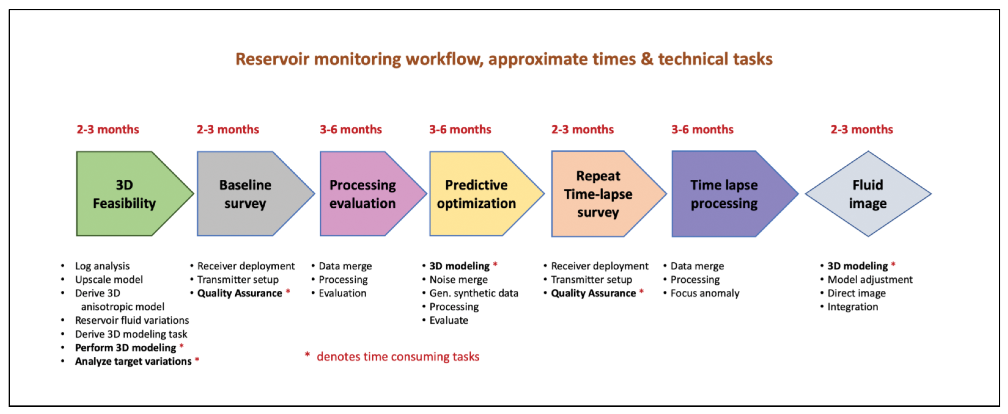
Figure 1 shows the workflow for EM reservoir monitoring, including technical tasks, and shows which tasks are the most time consuming. On average the time between repeat surveys is approximately 15–18 months. The first step in the workflow is the 3D feasibility, during which we derive survey design and optimized system selection. The main task here is to build a 3D anisotropic model, to benchmark the 3D modeling tools to avoid false anomalies, and to run 3D models. The derivation and running of the models and their analysis takes the longest (more than 50% of the elapsed time).
During the data acquisition, most of the time is spent on moving of the equipment. Quality assurance is carried out in parallel to decide if a receiver site is of sufficient quality and can be moved, or whether the recording must continue. For every given day, this process can delay acquisition by the same amount. Quality assurance includes data processing, basic data interpretation, and applying various criteria to examine the data quality. Each of the criteria (like data error and signal length or behavior of the transmitter current) is controllable, but in combination they need to be prioritized. The time needed for a baseline survey can often be reduced by using more equipment and automating field operations. The next step includes the data processing and data evaluation, which again mostly depends on careful data administration and data processing that can mostly be further automated. After the data have been evaluated, local noise conditions are known, then the reservoir model and its electromagnetic response is better understood. Having more detailed a priori information makes it meaningful to further optimize for the next repeat survey. We usually add here a step, called predictive optimization, where 3D synthetic data are generated, and local noise is added to the data such that the next repeat survey can be simulated. This allows further survey parameter optimization to ensure better imaging. For the predictive optimization, we have again the 3D modeling time as the biggest elapsed time user. The next step when the time lapse data get converted to subsurface images includes straight forward processing that can be automated. The last step of producing a verified fluid image again includes time consuming 3D modeling. Throughout the workflow, 3D modeling, and quality assurance are the most time-consuming tasks and very critical. It would be worthwhile to address them in terms of how they can be made faster and easier using AI.
Before we review where AI is making the biggest impact in electromagnetics for reservoir monitoring, we need to understand where fluid imaging technology makes its contribution to carbon footprint reduction. After that, we describe methodology and instrument and where they fit in the Cloud-based acquisition. Then we focus on those parts that benefit most from Cloud enabling. Finally, we develop how Cloud-based AI can produce game changing technology and contribute to the carbon footprint reduction. This is underscored by some application examples.
2. Value Statement: Linking Carbon Footprint to Fluid Imaging
Reducing greenhouse gas emissions has become a primary need for the oil and gas industry and is reinforced by various national and international agreements. We analyze various parts in the hydrocarbon lifecycle to understand where our technology can make the biggest impact.
On the other hand, the energy needs of the world’s population are inescapable. In effect, the International Energy Agency [
10] sees that the demand for energy for the year 2040 will increase by 24% and fossil fuels will supply 74% of this demand, with a growth of 13%. The growth of renewable energy sources will reach 83%.
Hence, to continue hydrocarbon production requires changes (reduction of carbon footprint) to the exploration, production, and refining processes to reduce greenhouse gas emissions.
Approximately 90% of greenhouse gas emissions (CO
2, CH
4, N
2O) are produced in the downstream process. Only 10–20% of emissions are generated during exploration and extraction. Those emissions reach an average value of 10.3 gr per 1 MJ of crude oil produced [
11]. This value may vary depending on the type of hydrocarbon and the process used for its extraction.
Table 1 shows the typical emission values according to the types of hydrocarbons and the production stages [
12].
Geophysics can greatly contribute to reducing emissions by supporting cleaner energy production, such as optimizing secondary recovery production that requires flood fluid monitoring (thermal, waterflooding, CO2).
Likewise, geophysics contributes to the generation and production of clean energies such as geothermal energy, besides its contribution to its exploration.
An emerging hydrocarbon production technique that will greatly contribute to reducing emissions is the so-called EOR+ [
13]. EOR+ has a dual purpose in that it requires CO
2 capture and sequestration while at the same time part of this CO
2 can be used for enhanced recovery. As such, it is possible not only to reduce emissions by optimizing production, but also to create positive credits by sequestering the excess CO
2 captured from the atmosphere. This enhanced recovery technique requires detailed description of the reservoirs and monitoring of the CO
2 injection front. Both can be achieved with the application of EM methods.
In all these enhanced recovery processes (water, thermal, or CO2 flooding) the common denominator is the change in electrical resistivity that occurs in the reservoir fluids when water, steam, or CO2 are injected. These resistivity changes, caused by electron flow due to the fluid mobility and conductivity, are detectable with EM methods because in most cases there is a strong resistivity contrast between immobile and mobile fluids.
3. Workflows and Value of Electromagnetics for Fluid Imaging
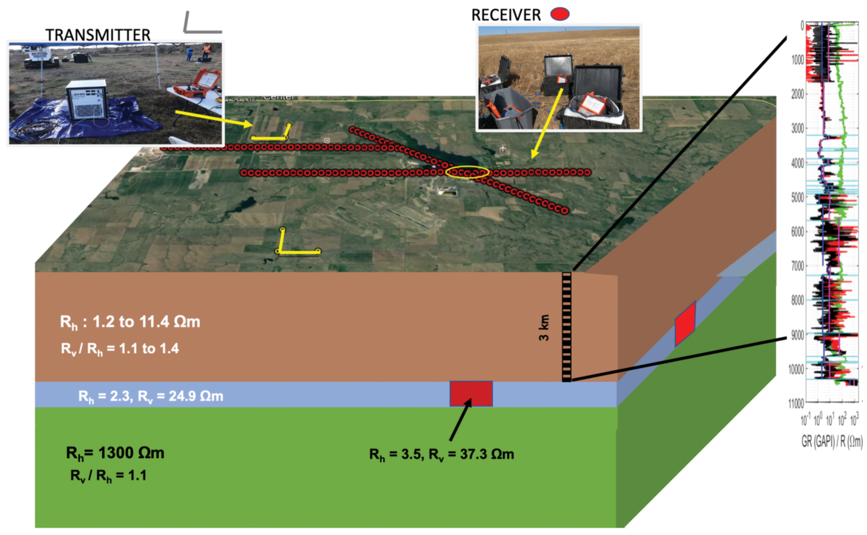
An electromagnetic system is laid out at the surface with transmitter and multiple receivers.
Figure 2 shows an example of such a layout where three receiver-lines are used to produce an area coverage. The transmitter in the figure is marked by the yellow lines (four transmitters in this figure). All receiver locations (shown as red circles in the figure) are used for each of the transmitters. Usually, before carrying out a survey, a feasibility study using 3D modeling is done to ensure that the survey setup can see target variations. For that, a resistivity log as shown on the right side of the figure is used. It is upscaled to determine an anisotropic model at a scale that can be resolved by surface measurements. This upscaled model is shown superimposed (blocky lines) on the log on the right: the upscaled horizontal resistivity are in blue and the vertical one in purple. The gamma ray log (GR) that is also in the figure is used to determine bed boundaries. The Earth model on the left shows an even more upscaled anisotropic resistivity model and indicates the target reservoir (marking the surface and side projections in the figure). In this model the target reservoir could either be the subject of enhanced oil recovery (EOR) or CO
2 injection. Through the transmitter we inject a current of desired waveform and the response from the induced current in the subsurface is sensed by the receivers at the surface. This process is repeated for several hours, and the recorded signals are averaged/stacked to get a better signal-to-noise ratio.
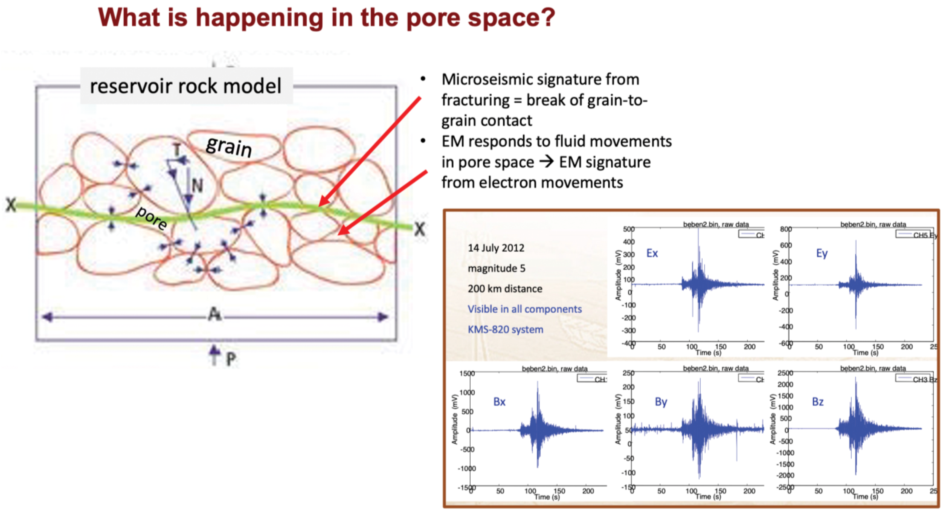
Since the biggest value of electromagnetics is in reservoir monitoring, we explain the petrophysics using a model of Carlson [
14] shown in
Figure 3. The rock is represented by grains and pores between them. Here, the fluids are in the pore volume and once stress or strain is experienced on the fluid it causes mobility of the fluid. This mobility makes the electrons in the water saturated fluid part move, thus resulting in drastic resistivity decrease. For earthquakes, we often observe that electromagnetic signals go along with seismic signals and appear slightly before the seismic signal onset because the breaking of the grain-to-grain contact comes after the rock experiences stress and the electrons move. We show an example from an incidental observation we obtained in India on the right side of
Figure 3. Here, we display the five components of the magnetotelluric field observed during the earthquake. The displayed time series speaks for itself as the earthquake is visible (time synchronous) on all data traces.
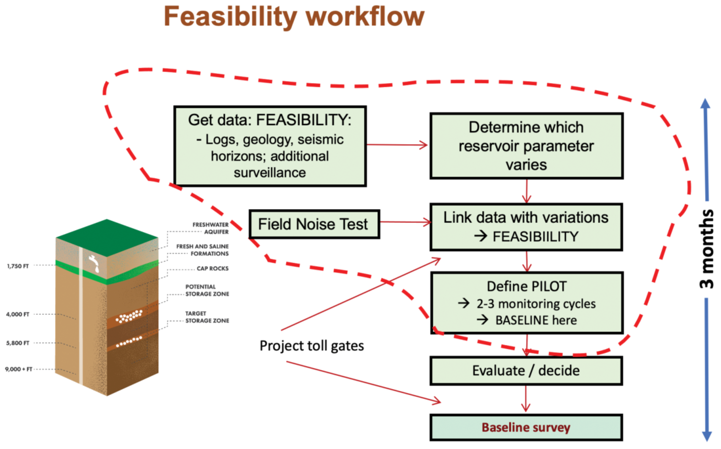
Since we attempt to measure our data better than with the accuracy of 0.5% (usual calibration variations that we observed are between 0.1–0.2%; maximum calibration deviation observed has been around 1.5%), careful survey design and optimized survey procedures are necessary. A feasibility study is in most cases mandatory, best even with additional local noise measurements. A workflow that we typically use is shown in
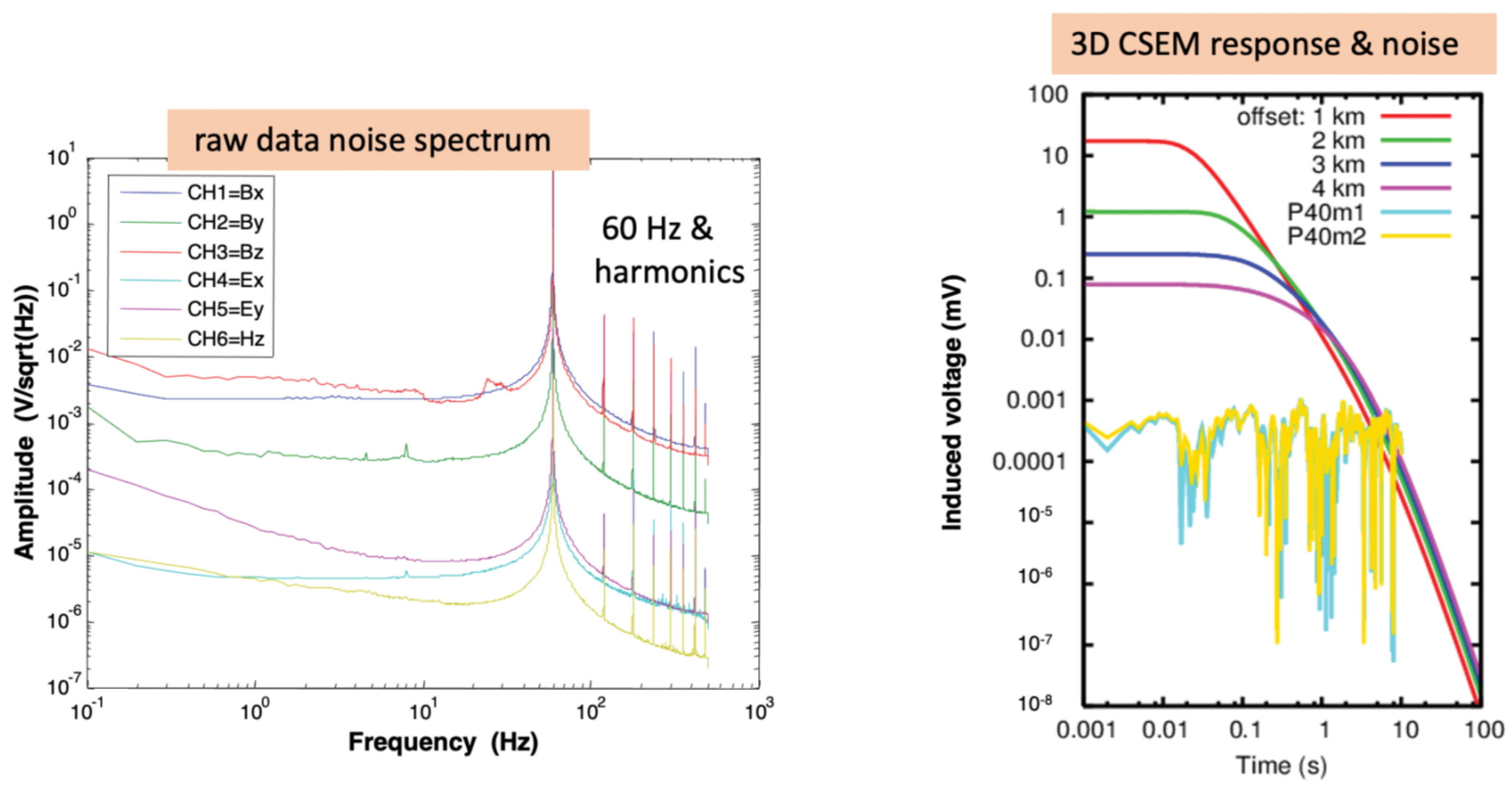
Figure 4. For monitoring application, we often look for less than 5% reservoir resistivity variation and we thus recommend a full 3D modeling feasibility study. A feasibility includes getting all available geoscientific data and carrying out a noise test on site. The data is then analyzed such that we preserve the target and define a range of target petrophysical parameter variation. These get translated to resistivity variation to define the modeling parameters and build a 3D anisotropic model derived from the most accurate information available. The 3D modeling results define future survey designs, leading to a baseline survey. An example for data building the data decision space one is shown in
Figure 5. On the left we see the noise spectra for the various sensors (electric and magnetic fields). On the right there are the 3D measured voltages induced in the receiver for various offsets. When we superimpose the noise spectrum as done in
Figure 5, we need to stay with our survey design parameters (offset, gains, and recording times) above the noise level. For that reason, the superimposed noise was filtered earlier to simulate realistic situations.
From this we determine recording time and select sensors, survey layout, and other operational parameters. Receiver spacings are derived by simulating the receiver response with different spacings. We simulate the time lapse by substituting the fluid in the reservoir model and estimating if we can reconstruct the anomalous reservoir.
During the feasibility the most time-consuming part is the 3D modeling (compare
Figure 1) and should thus be enhanced by using artificial intelligence, as will be discussed below.
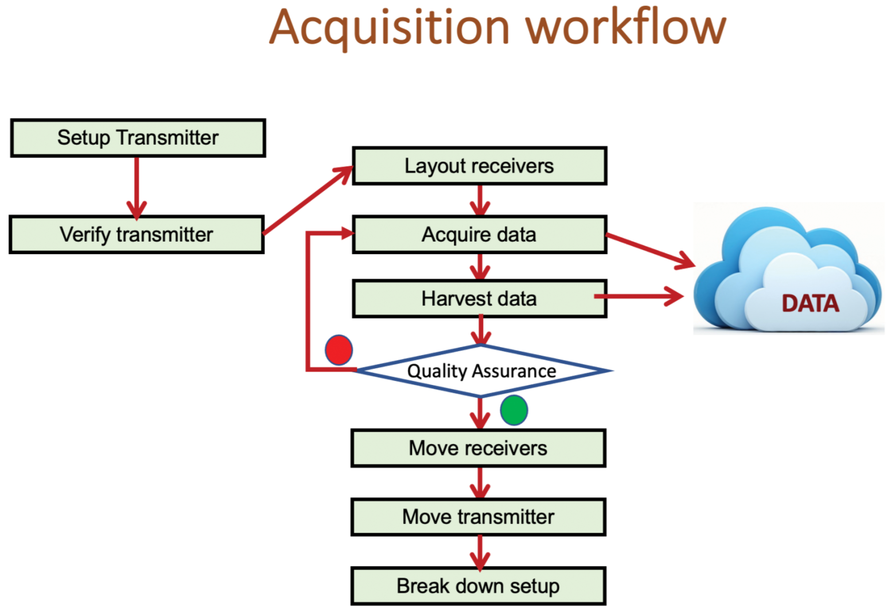
Next, we will review the acquisition workflow. Data acquisition is usually an expensive part of a project and requires careful timing and preparation.
Figure 6 shows a typical flow diagram for field data acquisition. A potentially time-consuming step is the quality assurance (QA) which is done concurrent to the acquisition. Here, the decision must be made whether a receiver is picked up and moved or remains on the ground to get better data (or needs to be improved). Thus, getting the data from the receivers to the QA specialist is important. We do this via a noise-free web access box which streams the data to the internet. This allows near real-time QA decision.
4. Background Enabling Instrumentation
The electromagnetic signals that we measure to obtain information of the subsurface are very small (tens to several hundred pT) and they need to be measured in the presence of an Earth’s magnetic field (25,000–65,000 nT) that is 1 million time bigger. In addition, we have external noise and man-made noise that can be more than 1000 times larger than the Earth’s magnetic field. It is a difficult task but it is not impossible, and is customary to geophysics/military/space science. Our sensors have such high sensitivity that they cannot be easily integrated with other data transmitting devices such as cell phones as they generate too much noise for the sensor and distort the signal. For passive electromagnetics, this is because of the broadband sensitivity. So, often, data transmission is done during acquisition pauses. For CSEM, that is not easily possible because we require a very accurate reference voltage level which can only be obtained with continuous data acquisition.
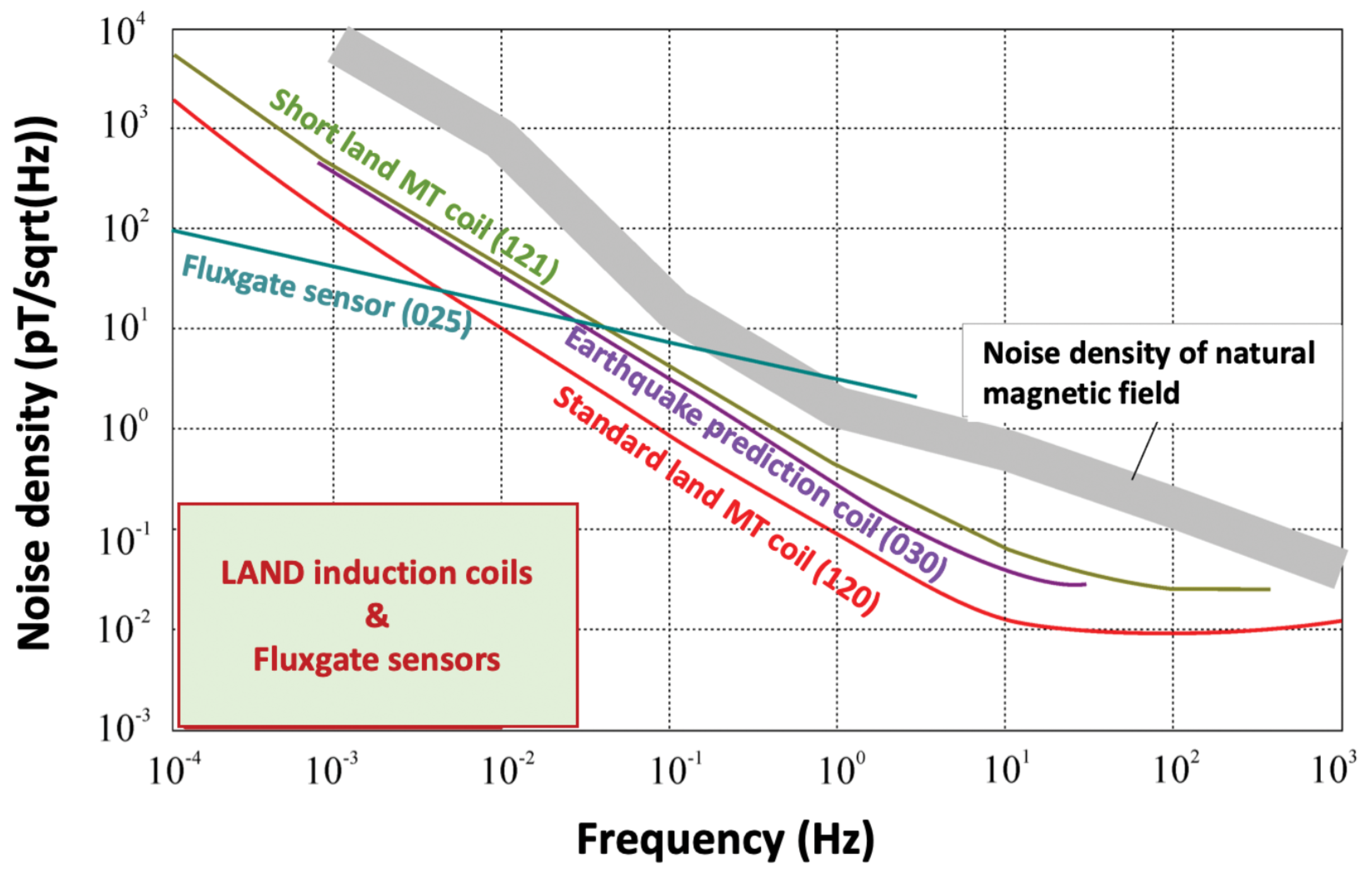
Figure 7 shows the typical noise density for various magnetic field sensors (the electric field sensors have different, less critical, issues) used for land geophysical methods discussed here. In comparison we also plotted the noise density for an earthquake prediction coil and the noise density of the natural magnetic fields. All sensors must be below that noise level. We solve this issue by jumping via a low-noise Wi-Fi connection a short distance away from sensors and all analog parts into a web access box where the data are buffered and then sent to the internet with various protocols. Further discussion is in the section below.
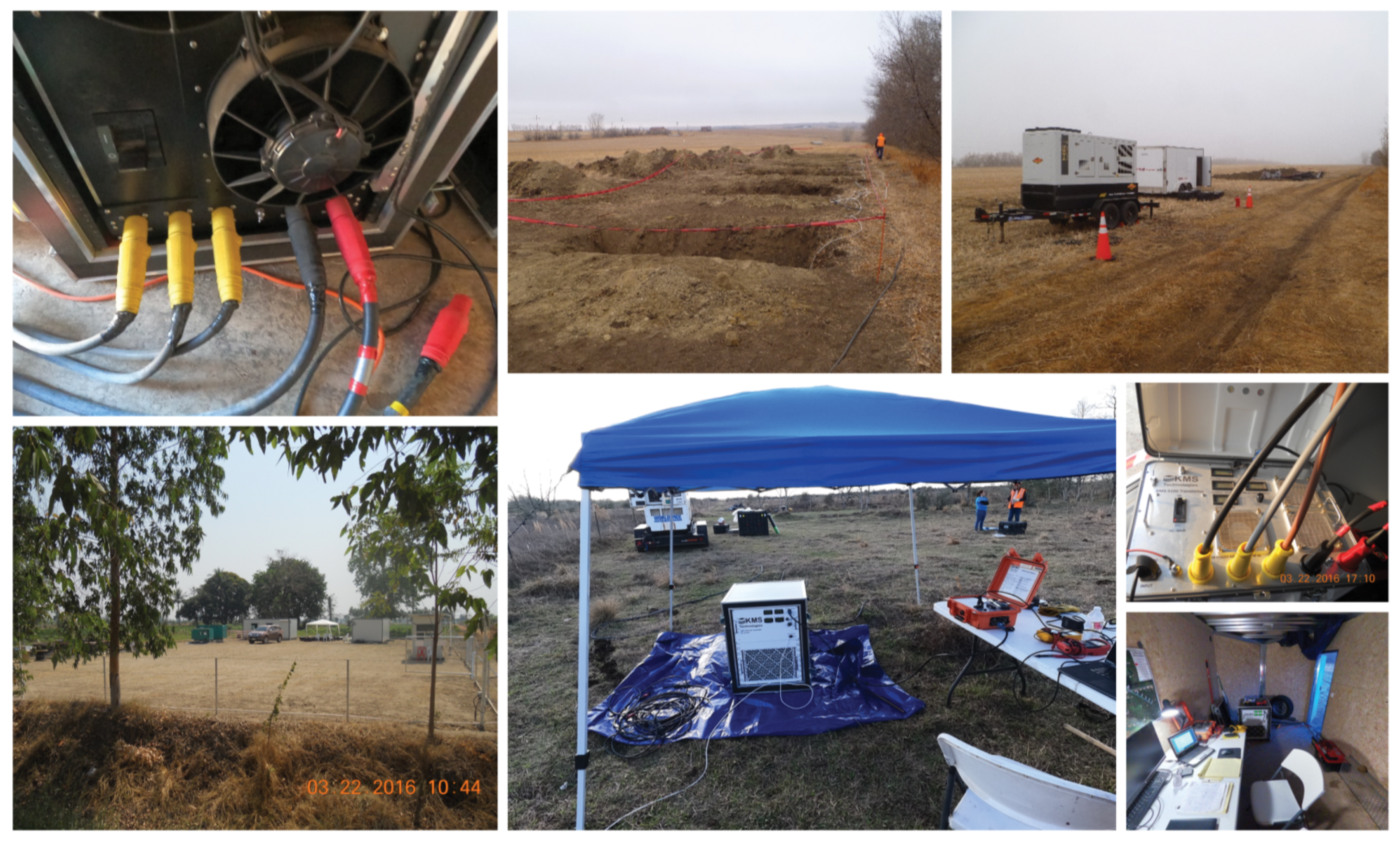
Figure 8 shows field pictures of various receiver equipment components. Our target depth is between 500 m to 6 km in almost any geologic environment for a variety of applications from geothermal, carbon storage, to hydrocarbon applications. At each of the sites multi-component EM equipment is deployed to measure either magnetotelluric (MT) or controlled source electromagnetics (CSEM) response. We use ultra-stable electrodes for the electric field that have a broadband response from close to DC (better than <0.0001 Hz) to about 40 kHz on the high end. Stability of the sensors at the low frequency end is essential for fidelity of the signal and to determine the proper reference voltage. It should be noted that capacitive electrodes are not suitable as they do not go low enough in frequency to cover that depth range. At the top left of
Figure 8 we show the electrode we used, which is a lead-free LEMI-701. The electrode spacing is either 50 or 100 m. Magnetic field measurements can be done by either fluxgate sensors, induction coils (center photo in
Figure 8), or air loop (bottom left photo). We test all of them at each survey location and compare its noise with the local noise to optimize layout and acquisition times including operational deployment. Pictures of the acquisition system we use (KMS-820 array system) are shown in the other three photographs in the figure. The yellow box in the picture on the top right is the web access box that allows data streaming to the Cloud. It is important to note that the acquisition system must operate from −20 °C to 60 °C, acquire continuous data for weeks at a time, and be connectable to the Cloud.
Figure 9 shows various transmitter photographs under field conditions. The transmitter consists of a generator, a current switchbox, and a waveform controller that records the transmitter signals and is GPS synchronized. On the top left and the center bottom of the figure are pictures of our 150 kVA (KMS-5100-150) switchbox, back and front side, respectively. The switchbox converts the alternating current from the generator to direct current and switches it according to a predefined waveform (usually a square wave). This current (up to 400 A) is injected into the ground via large grounding electrode plates placed into pits on both sides of an approximately 1 km long thick cable. A picture of four pits (one dipole side) is shown in the top center of
Figure 9. Further transmitter site picture is shown in the top right (generator and observer trailer on the top right) and in the bottom left a camp site in an oil field. In
Figure 9, center right, is a picture of the 100 KVA version of the switch box and below on the right an inside view of the recording trailer.
The most important element in all of this is to send the data in real time to the Cloud. Where cellular phone coverage is available this can be done via cell phone.
After describing the instrument [
15], we need to consider the methods and what they are used for. The most mature electromagnetic method is magnetotellurics (MT) as described in [
16,
17,
18,
19]. MT is the primary method for geothermal applications but also used to limited extend for hydrocarbon and other academic applications. MT uses the Earth’s natural field, and the signal can be improved by adding a signal to the weak band. In that mode the method is known as controlled source audiomagnetotellurics or CSAMT [
20]. An even better coupling to the resistivity of the subsurface is obtained when the equipment is used in controlled source electromagnetics (CSEM) mode (in time or frequency domain) [
20,
21,
22,
23]. The problem with CSEM is that the image focus is unknown. This can be improved by using focusing methods like the borehole-logging-style focusing described by Rylinskaya and Davydycheva [
24]. Using such a system for a combination of methods including boreholes is described by He et al. [
25] and Strack [
26] and for marine applications by Constable [
27]. The choice of methodology is determined by finding the optimum solution using the 3D feasibility approach described above.
5. Converting the Workflow to Cloud-Based Application
Going from concept to real data implementation requires that the turn-around time of all the tasks in
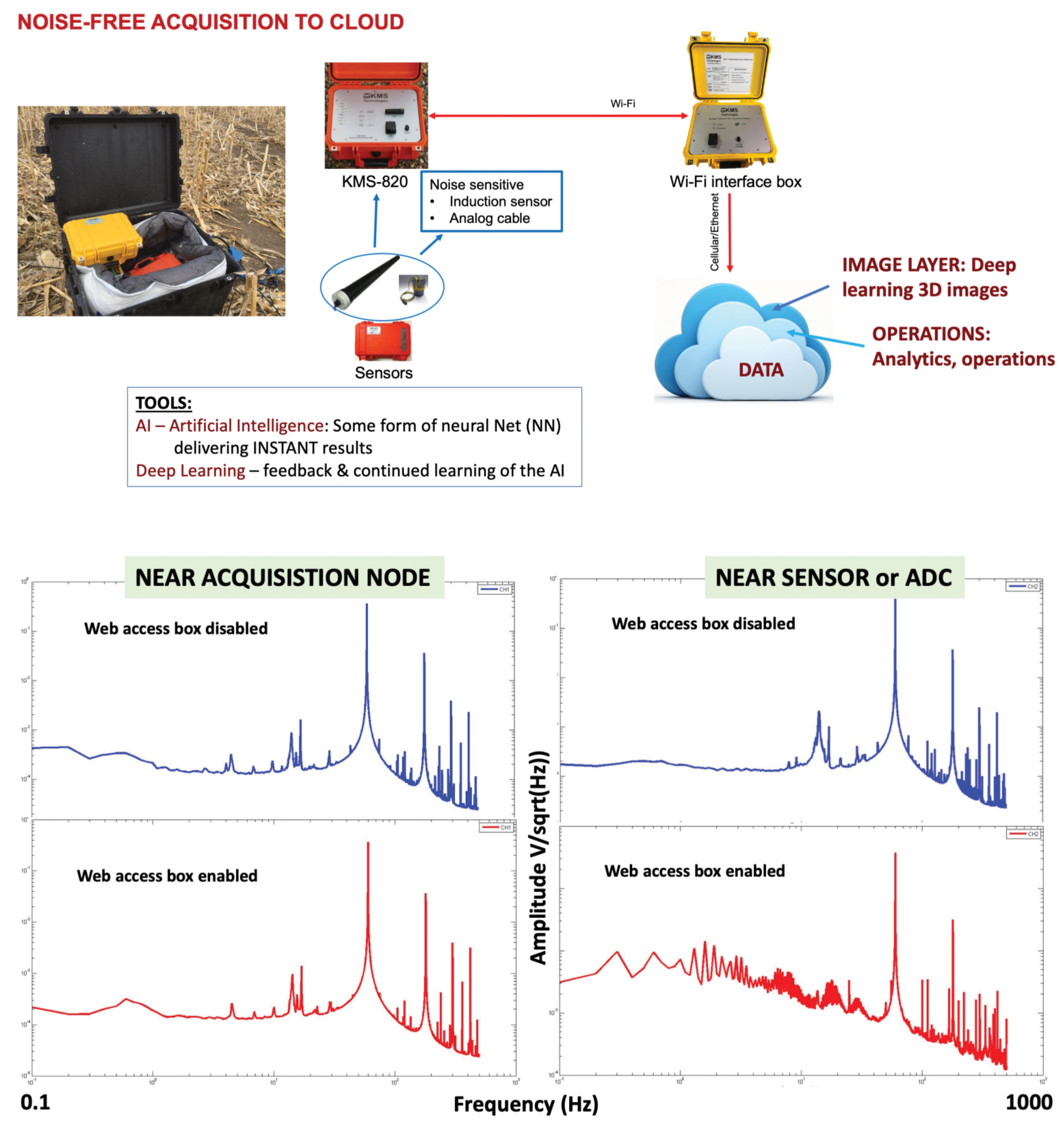
Figure 1 be reduced to near real time. We started to address the most time-consuming ones and to illustrate their progress to show its uniqueness. To appreciate the difficulty of the proposed undertaking, on the path to our goal—a fully distributed autonomous system where sensors, acquisition, and Cloud data transfer are near real time operations—we still need to understand small electromagnetic signals and their sensitivity to external noise, natural or man-made. To separate between data for storage/transmittal purposes, service support, and deep learning related analytics we separated the Cloud into three layers as shown in
Figure 10: the DATA layer, which is mostly for data transmission and archival purposes; the OPERATIONS layer, where interaction between acquisition unit and user occurs; and the IMAGE layer, where the information is interpreted and improved using deep learning algorithms. In the OPERATIONS layer, feedback between acquisition unit and the user also occurs. When the web access box is placed away from the sensor both respective curves are very similar (left of bottom of
Figure 10). Clearly, the web-access box generates little to no extra noise and let us realize the value of having the field data available in real time. It should be mentioned that for magnetotelluric data it is important to separate the acquisition unit from the web access box by a few meters. Only by avoiding the data transmission noise can you acquire true continuous time series which is essential for several data processing steps.
In practice, the most difficult part in this is the cell phone coverage and good data transfer. While replacing of the Sim card should be the standard, we experience a lot of inconsistency between cell phone providers around the globe and must work in most cases with their technician to make this work. Hopefully, once satellite-based internet is commonly available, this will become history even in the remote area where often geophysics is applied.
Operationally, having the data available in near real time in the Cloud is not only a huge time and thus money saver, but also an enabler. We can now do many things and apply the technology to problems hereto impossible. Collaboration between staff on site and the experts located half a globe away is much more immediate and beneficial not only during problem solving instances. An obvious advantage is that the data can be processed quickly while the equipment is still laid out on the ground. Another major cost saver can be obtained when safety/security training and licenses are required from the acquisition personal but not from remote personal and when extreme weather conditions existing from cold (−20 °C as used during the data acquisition shown here) to heat (+50 °C as often during our field testing).
It is an enabling operational benefit to have the instruments deliver the data in real time. For Reservoir Monitoring (which we determined is the highest value for electromagnetics in the future path to Zero footprint), we need to look at the most time critical task indicated in
Figure 1. During the 3D feasibility step (workflow shown in
Figure 4), 3D modeling is the most time consuming, while the analysis of the results only requires more experience to automate the process in the operation Cloud layer.
Usually, when we think about 3D modeling and data we think about inversion because we are trying to derive an Earth model from the data. Because our field measurements contain noise, and our methods are partially multi-valued, we cannot always provide a unique inverse solution [
21]. When we analyzed this problem with borehole resistivity logs in the 1990 [
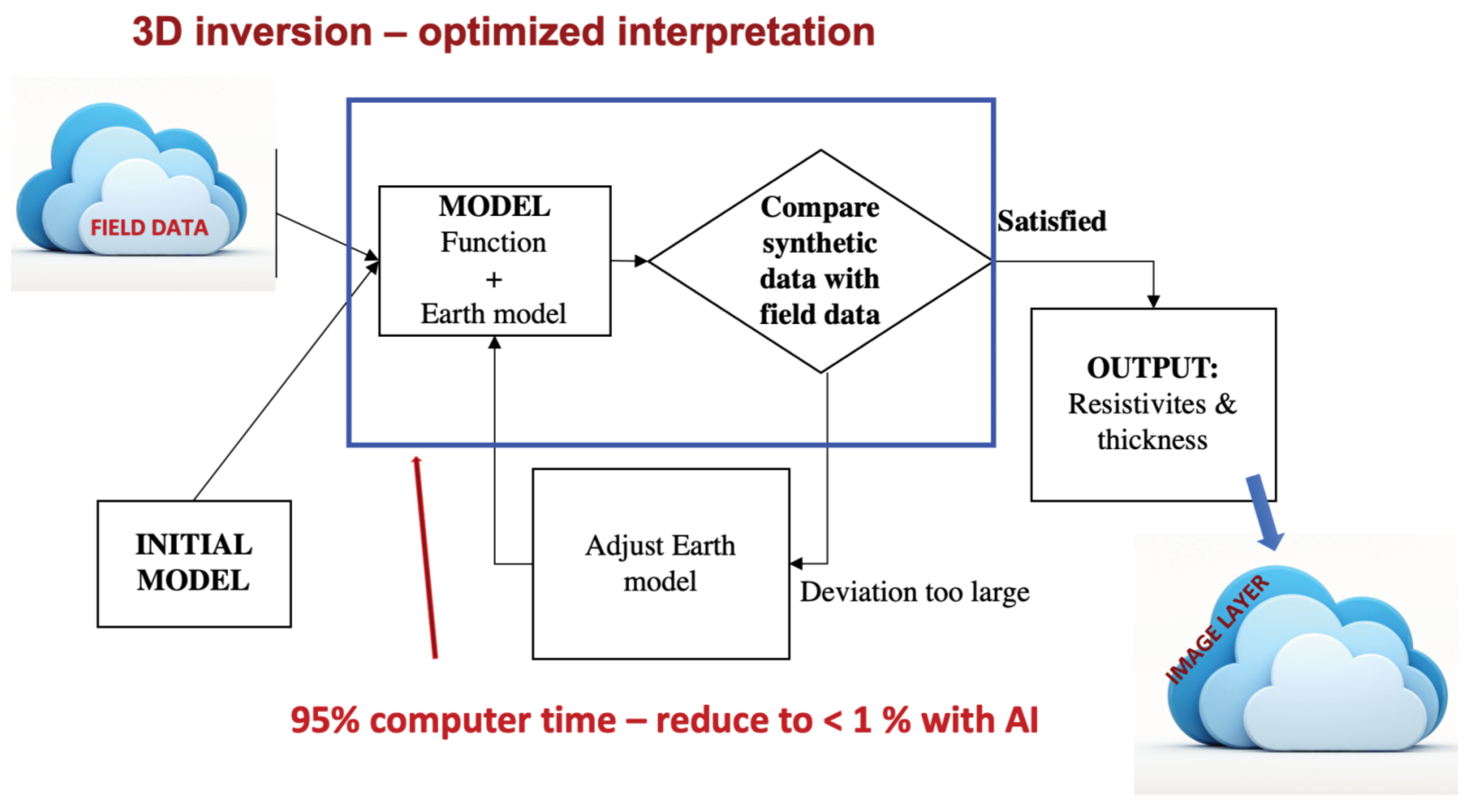
28,
29], we noticed that 95% of the computing resources were spent on the 3D forward model, which has a unique solution. So, instead of using the neural net for the inversion, it was more effective for the forward models [
30], where it also can save up to 95% of the computing time. Subsequent substitution neural net based forward modeling reduces the inversion elapse CPU time by 92%. When replacing forward models with neural nets, we must realize that EM responses depend on resistivity contrast and the conductance or transverse resistance of the specific reservoir unit. This is often called equivalence in electromagnetics. This has fundamental implications as resistivity profiles are usually specific for each specific basin (or formation analogue). Not only do we need to train artificial intelligence-based algorithm for each basin (or geologic analogue) but also with many training sets (tens of thousands).
Figure 11 describes the inversion components for electromagnetics. In the forward modeling the Earth model (1D or 3D) gets combined by the forward modeling function and model responses are generated. These are then compared with the real data and, if they match, we have found a realistic model explaining the data. Since they usually do not match in the initial iterations, the forward modeling is done many times and thus becomes the 95% CPU time user. Forward modeling can easily be substituted by artificial neural networks. The input to inversion is the data from the Cloud data layer and the output would go to the image layer.
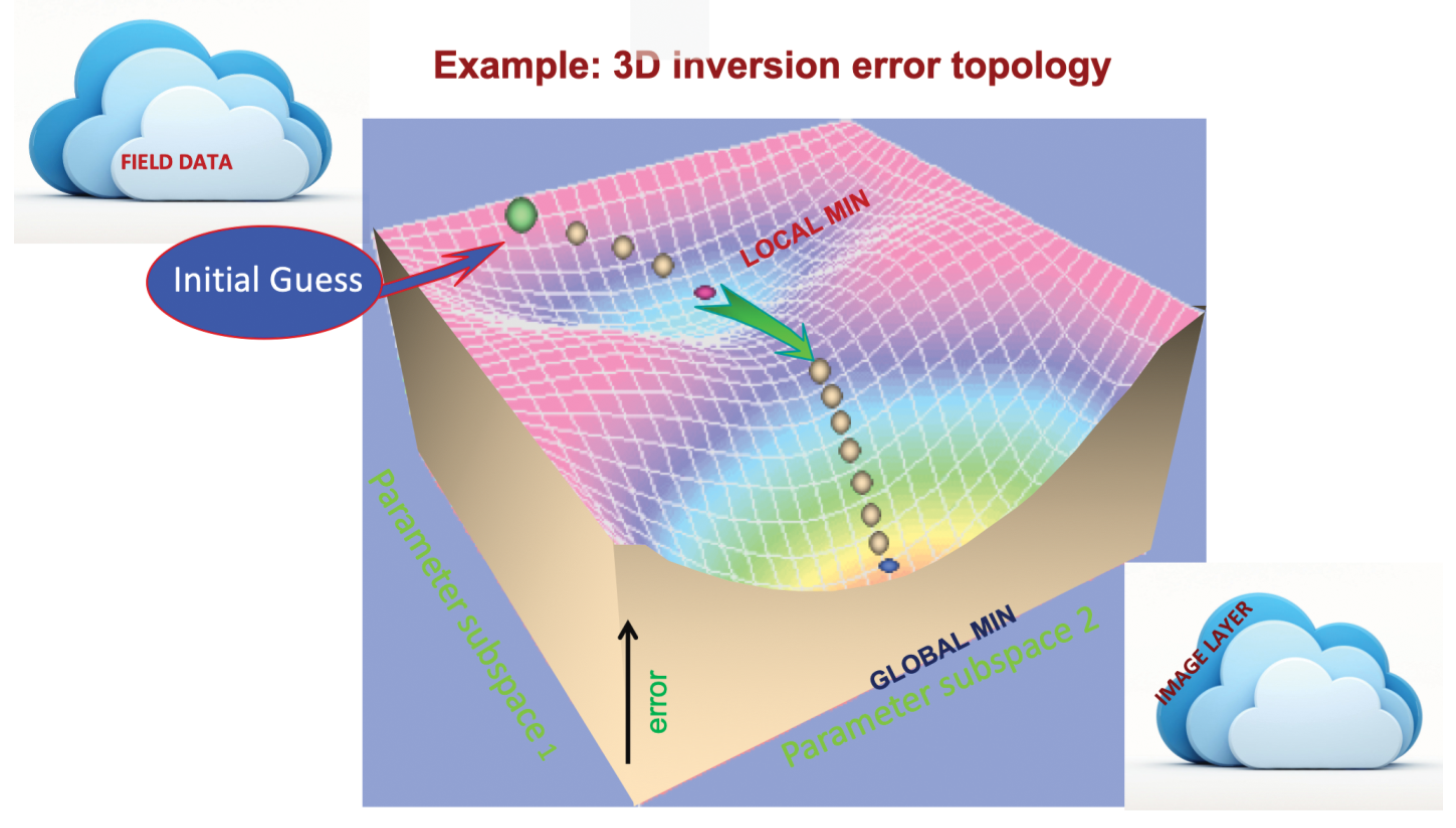
Figure 12 explains why we do not recommend substituting the inversion (better model match/updating) with a neural net. In the figure we have two parameters space that represent the model or transformed parameter space [
21]. For a typical 30-layer modeling we have 29-layer parameter (one-dimensional) or 293 parameters in the three-dimensional case plus various vector anisotropies. Because electromagnetics often responds to conductance (thickness time conductivity product) or transverse resistance (resistivity time thickness product), we cannot always separate parameter combinations and obtain error surfaces, as in
Figure 12, that have local and global minima. As geophysicists, we always look for the global minimum (as the best solution), which may not always be the right thing to do from the explorationist (geologist) viewpoint when you try to get a consistent model with most data sites and can tolerate higher curve fitting errors. That decision between local and global minimum is not easy as it requires understanding of all data sets and geology.
6. Implementation Example
To illustrate how we transition to using artificial intelligence, we apply the above-mentioned principles to the instrumentation and deliver the data directly to the Cloud. In
Figure 1 we describe the most time-consuming parts in each workflow step. Here, we select some of them to illustrate the value of the implementation.
Obviously, the Cloud usage as data delivery and depository vehicle saves a lot of time/money.
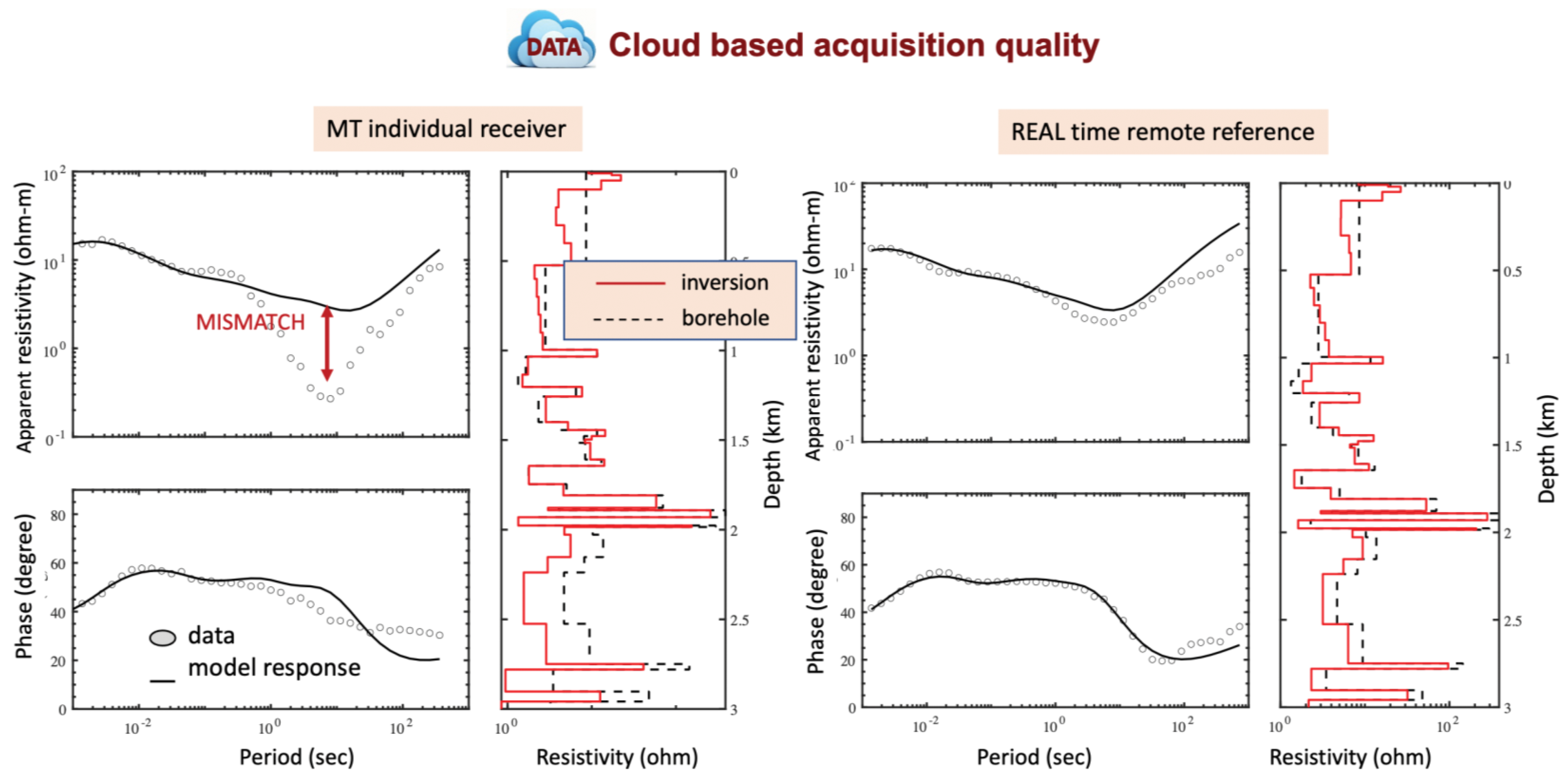
Figure 13 shows an example of electromagnetic data (here MT data) where the Cloud enables us to combine data sets acquired thousands of miles apart. We acquired a large set of MT data in the Northern USA and used two remote reference sites [
17], one in the northern USA 600 km away from the survey area and another in the southern USA about 3000 km away. Using the Cloud allows us to utilize interpretation resources far away and take advantage of different time zones. In this case the data acquisition was done in northern USA at −20 °C at two locations and around 50 °C at the southern US location, where the instruments were field tested. The interpretation was done in Europe (Sweden and Germany) and Texas. The results were available within 24 h. This would not have been possible without the noise-free web access as described above.
Figure 13 shows the results and comparison between using a single site and including a remote reference site. In the individual site processing on the left, we still see a significant mismatch over a wide frequency band. When including the remote reference site for noise compensation, this mismatch goes away as we get a more realistic data/model match. To the right of the curves are the Earth models obtained from the inversion (dashed) and the one derived using upscaling of the resistivity log shown in
Figure 2. The inversion model matches the log well which is the basis for our judgement. The value in this is multi-fold:
Significant interpretation time saving.
For operations purposes, we more easily determine whether a site must be repeated or the quality is sufficient.
Significant confidence increase in the 3D feasibility subsurface model reduces interpretation time.
As a next step, we developed a deep learning artificial neural network to assist our data quality assurance (QA) effort, mostly because the turn-around time of the quality assessment can be very costly for operations. If we can implement artificial neural network to assist QA process, it will save us tremendous operation time. This is part of NOISE-FREE acquisition to cloud, which is explained in
Figure 10. To automate and improve QA process, we introduce deep learning artificial neural network and implement the process in three steps: STEP 1. Set up a dedicated server to automatically harvest each data set from the Cloud; STEP 2. Run artificial neural network to derive instant QA result; STEP 3. Feedback to operator and add results to the operations Cloud layer. The success of this implementation relies on building a suitable artificial neural network and get it trained by deep learning method [
31,
32,
33]. For illustration purposes we illustrate here the initial artificial neural network and deep learning phase.
To build an artificial neural network we need to derive input parameters that represent the data, the scientific processes applied to the data like processing or inversion, and the human interaction with the data (like operational behavior or model objectives). This seems initially simple if we manage to use clear technical metrics to evaluate each of the areas. Data QA comes from acquisition observation, raw data curve behaviors, and 1D inversion results. Since we had an accurate anisotropic borehole log derived model, the inversion match overrides acquisition quality (in this example only). Thus, we define two levels of QA parameters: Level 1 is based on acquisition observation and raw data curve behaviors; Level 2 is based on 1D inversion results. To simplify, we use QA 1 to refer to QA parameter Level 1, and QA 2 refers to QA parameter Level 2. In QA 1, MT curves are evaluated within the frequency range from 0.001 to 1000 Hz. QA 1 contains robust processing parameters [
34]: root mean square (RMS) error, phase behavior, and apparent resistivity. QA 1 was set to classify each curve into 4 levels:
Level 1—Excellent, ≥85% of data points have a relative error (standard deviation (SD) of Amplitude/Amplitude; absolute error of phase = 0.56 relative error for amplitude) <10% and with smooth continuity.
Level 2—Good—more than 75% of data point (in period) have a relative error <20%.
Level 3—Acceptable—Phase does not go out of a quadrant (0–90°) (minimum) and amplitude of impedance tensor does not go down more than 45° and it is not increasing with period.
Level 4—Poor, data points show large dispersants, and it is impossible to define a curve for interpretation.
Further categorization is possible based on the impedance tensor (main components) and will be implemented in future deep learning practice.
In QA 2, 1D Inversion quality criteria—override (if inversion quality is better than acquisition quality including remote reference is taken precedence):
Level 1—Excellent, data fitting has a normalized root mean square fit (RMSf) ≤ 2.
Level 2—Good, 1D fitting has a normalized root mean square fit (RMSf) > 2 and ≤5.
Level 3—Acceptable, 1D data fitting has a normalized root mean square fit (RMSf) > 5 and ≤10.
Level 4—Poor, 1D data fitting has a normalized root mean square fit (RMSf) > 10.
We use normalized RMS fit which is RMS (fit between predicted observed)/SD to fit the data within 1: i.e., fits the data within standard error bars [
18,
34].
A deep learning algorithm can learn patterns from data sets. During an MT project in the US, we acquired about 250 data sets in 50 stations. We are using this data in two steps: training and testing steps. Deep learning programs train themselves through training data and test accuracy of the algorithm via testing data. Improvements which yield lower value impact are smaller in the operational context where the decision ‘repeat measurements or move receiver equipment’ must be made.
Our deep learning module has two parts: artificial neural network and statistical quality control module. An artificial neural network predicts QA result and the quality control module remove outlier from predicted QA results. To construct a deep learning module, we randomly selected 37 data sets as training data and rest of the data sets were testing data. For each training data set, we randomly defined a predicted QA result to simulate of the output of artificial neural network, and the predicted result was compared with the actual QA result (produced by experienced geophysicist). After the comparison, we took the difference between predicted QA result and actual QA result and then calculate the difference ratio, which is difference divides actual QA result. The difference and difference ratio are used as input value to a statistical quality control module [
35] to train the neural network. This statistical quality control model is based on theory of central limit theorem [
35], it removes outlier of predicted QA when training neural network and improves it.
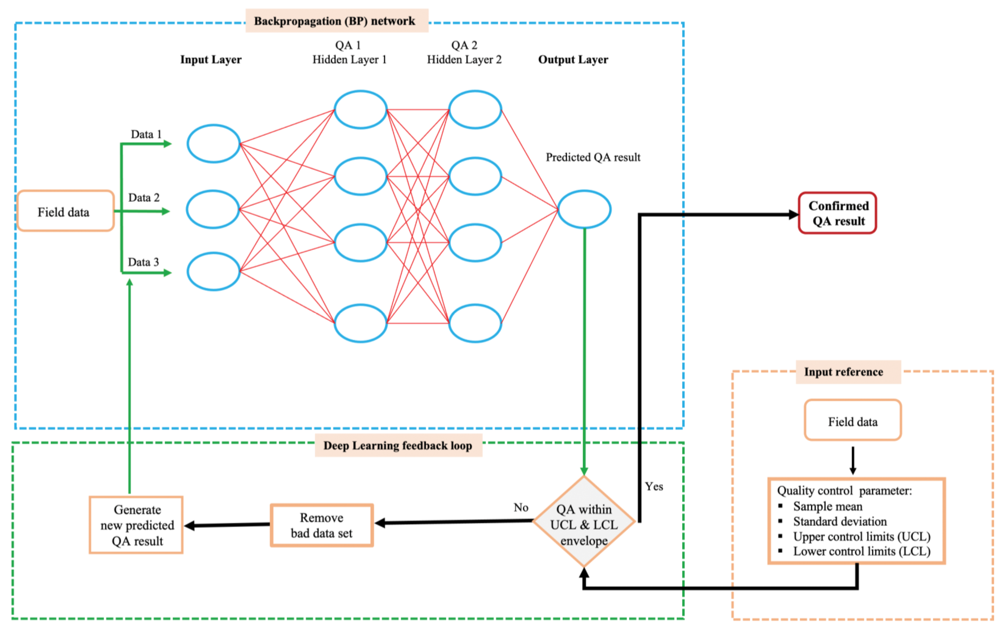
Figure 14 shows Backpropagation (BP) artificial neural network (top left) in this application [
36], input layer reference (top right), and deep learning feedback loop (bottom). Input data go directly to the artificial neural network, and this artificial neural network predicts the QA result. We also created a statistical quality control module to evaluate and improve artificial network predicted QA results. We chose BP network because of its efficiency over other algorithms. In the BP network, three input nodes are global positions satellite (GPS) information (Data 1 including coordinates, time, and altitude), instrument amplifier gain settings (Data 2 including acquisition unit amplifier settings for each channel), and operator’s name from each data sets (Data 3); two hidden layers are QA 1 (QA parameter Level 1) and QA 2 (QA parameter Level 2); One output node is predicted QA result. The predicted QA result will get compared with the actual QA result, which was produced by an experienced geophysicist. The comparison is quality controlled by central limit theorem algorithm [
37], which is explained below. By feeding back comparison results to BP network, it is getting trained continuously and the deep learning cycle starts. The more data sets we provide to this BP network, the better it performs.
To improve our BP artificial network, we need to establish a statistical quality control module [
35] to fine-tune deep learning predicted results. Artificial neural network predicted results, especially at the beginning stage, will have large error rate. We set up an outlier detection algorithm based on central limit theorem [
37]. The workflow of quality control module is shown in
Figure 14 (right side). The quality control module algorithm is explained in
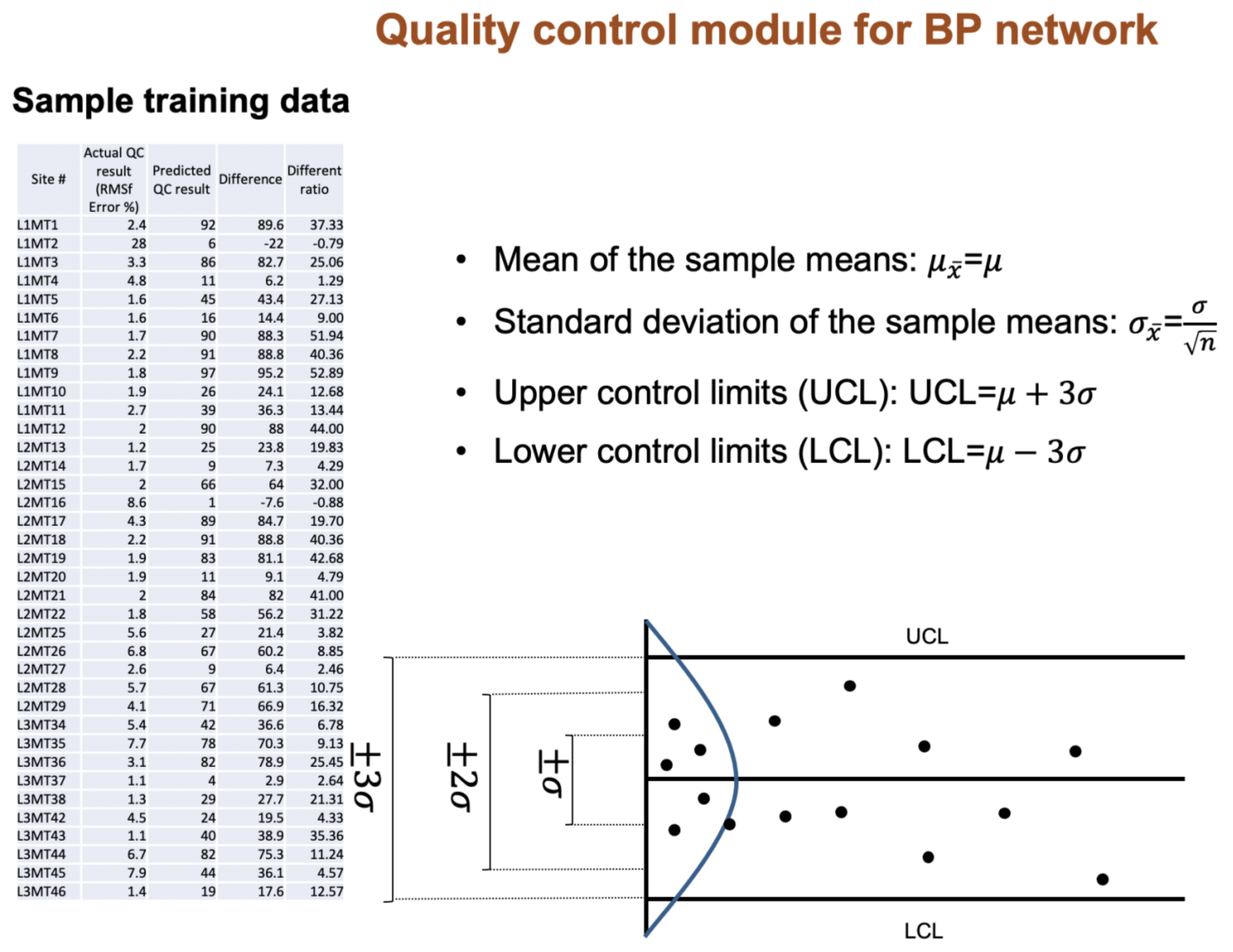
Figure 15.
The
Difference for the data set means the difference between
Predicted QA result and
Actual QA result (Equation (1)), and
Difference Ratio is difference divides
Actual QA result (Equation (2)).
According to central limit theorem, the following four properties are needed and calculated from sample training data sets:
Mean of sample (
) mean equals to the mean of whole data sets:
The standard deviation (SD) of the sample (
) equals the deviation of whole data set divided by square root of the sample size:
We assume the original data sets are normally distributed; therefore, the sample means will be normally distributed.
If, in any case, the distribution of original data sets is not normal, a sample size of 30 or more is needed to use a normal distribution to approximate the distribution of the sample means. The larger the sample, the better the approximation will be.
We selected 37 sample data sets shown in
Figure 15 (left) as initial input to quality control module for network. The data are selected from all stations (remaining data showed high cultural noise). Each data set has an initial (random)
Predicted QA result. According to central limit theorem [
37], we calculate mean of the sample means
, and standard deviation of sample mean
. We defined upper control limits (UCL) as well as lower control limits (LCL). The limit is range within
, which is from −54.24 to 93.42. When we start feeding our training data sets to BP artificial network, if the difference ratio of one data set is outside of the range (−54.24–93.42), we consider this data set an outlier, and it will be removed. According to our test, the range defined by UCL and LCL covers 99% of predicted results but it can still remove outliers. By implementing this central limit theorem as a quality control module, all the data points outside of limit range are considered outliers and removed. With this quality control module in place, our BP network gets trained to produce better
Predicted QA results. As we feed more training data sets to BP network our deep learning neural network will get better to produce instant
Predicted QA results.
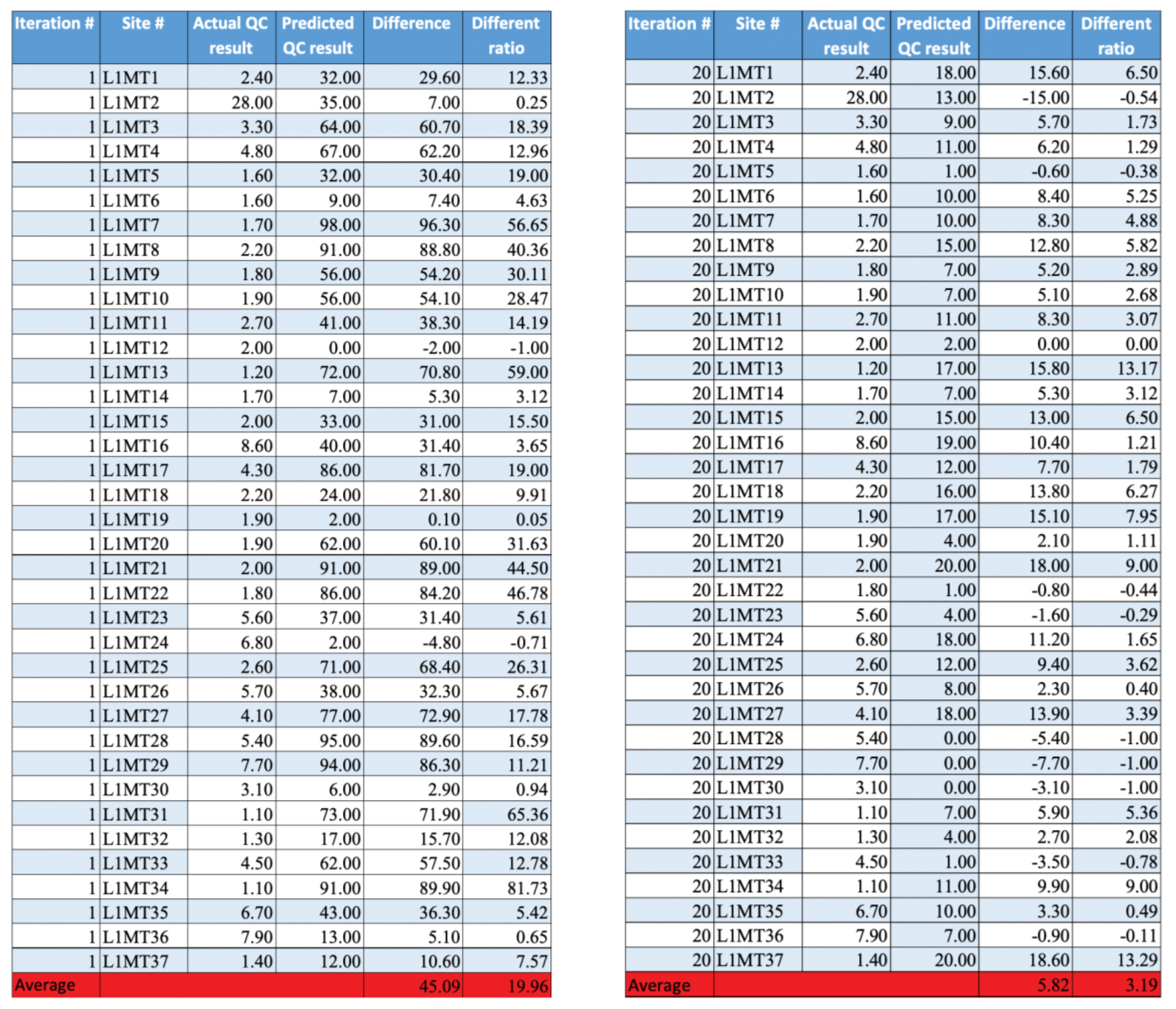
Once the quality control model for our BP artificial network is set up, we started feeding it with data to train it. We randomly selected data sets of 37 stations (one data set from each station, exactly same amount of data sets as our initial sample data sets). BP network training process takes time, especially at the beginning stage. By feeding training data sets into the BP network in multiple iterations, we expect to get better predicted QA results gradually. As shown in
Figure 16, training results of first iteration (table on the left in
Figure 16) shows average difference is 45.09 and average different ration is 19.96. After 10 iterations, training results turns out to be average difference of 5.82 and average different ratio of 3.19. From this comparison, we can see there is about 84% improvement of predicted QA results after 20 iterations of training. Since we are continuously feeding more training data sets to our BP network, better predicted QA results will be produced. As we must make operational decisions with a fast turnaround time, we declare the network after 80% improvements to be operational.
Our work combined deep learning neural networks and statistical quality control module to make fast turnaround predication of MT QA results. So far this method has already shown us that it has great potential to reduce field geophysicist workload and significantly improve efficiency of field operation in terms of data quality feedback. As part of our cloud acquisition workflow, we continue to train our BP network to produce faster and better predicted QA results. Meanwhile, we are also adding fully automated features to have these QA results delivered to field crew’s fingertips simultaneously. This will significantly improve field operation decision making process, make field logistics more efficient, and thus reduce operational cost effectively.
We have discussed using AI in data delivery and quality assurance: both tasks are very time consuming and costly. We also outlined the roadmap for effective implementation in 3D modeling, as an illustrative example we looked at the value the Cloud enabled, AI supported technology provides by looking at its enabling capability in predictive optimization and performing repeat time-lapse surveys. During the energy transition a high value target for GHG reduction are heavy oil (HO) applications to EOR. We have taken a typical HO example which includes a shallow reservoir which is of near-term concern but also environmentally sensitive due to its shallow depth. Without the above-described technology and workflows this application would be extremely difficult to accomplish. With it we can apply new technologies that we explain forthcoming.
The production of HO can produce up to 715 kg CO2e/bbl from upstream to downstream, of which 10 kg CO2e/bbl are released when thermal methods are applied. Monitoring of steam injected becomes extremely critical to lower the number of emissions. Resistivity can change up to 150% for a temperature increase of 100 °C.
Several feasibility studies were carried out in the last decade [
38,
39] and we present below selective results one of these in this context.
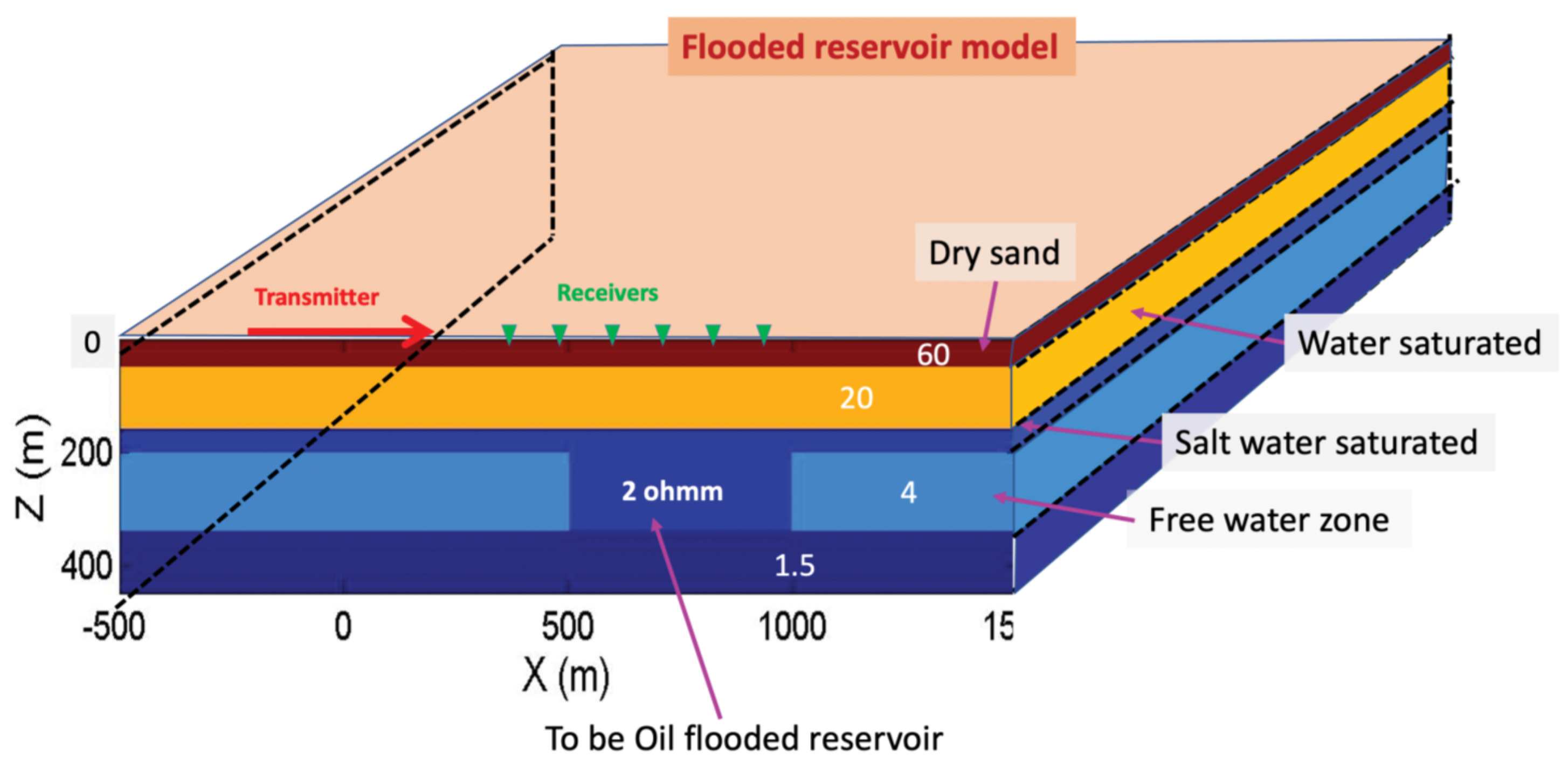
Figure 17 shows the geologic section of a representative heavy oil field. Depending on the resistivity contrast between the fluids in the reservoir we will use different EM sensors. Simultaneous microseismic data are also acquired to monitor the changes of pressure occurring in the reservoir due to the injection of steam on one side. On the other side this will be used to observe potential breaks of the reservoir seals. In the figure we show the resistivity model of the formations and the saturation fluid description. Additionally shown is the CSEM survey configuration. We did not show the anisotropic model to avoid distraction from the purpose here on improving image focus and delivering the data in near real time.
We carried out a simulation of the EM responses using a 3D finite-difference method [
40] applying to the feasibility concepts described above and in [
21,
41]. In
Figure 18 we show the synthetic response of the offset-corrected horizontal electric field (Ex), for the isotropic (left) and the anisotropic case (right). We assumed here a vertical resistivity Rv = 8 ohm-m and a horizontal resistivity Rh = 4 ohm-m. Clearly, as expected, the anisotropy adds significantly to the anomaly. Henceforth, we will only use the anisotropic model. We also can see from this figure that the anomalous behavior or difference between flooded and unflooded reservoir is largest near the reservoir (outline at the bottom of the graphs). This suggests if we can get this difference out of the data using some type of transformation that only shows the variation between adjacent receivers, we might just see this [
41]. This is commonly done in focused borehole measurements and can be translated to surface electrical fields [
42,
43].
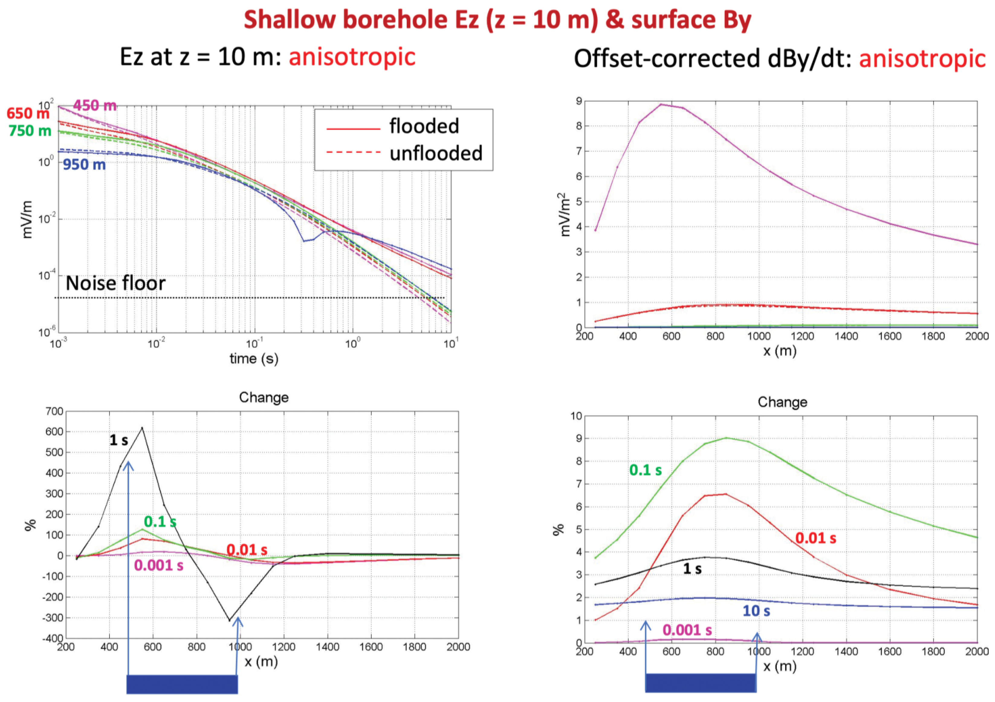
Figure 19 shows two other electromagnetic field components to achieve this anomaly enhancement: one is the measurement of the vertical field and one the measurement of the horizontal magnetic field time-derivative. The implementation of the vertical electric field measurement would happen via a shallow vertical borehole tool that gets buried in 20 m deep boreholes. This leads directly to the benefits of using artificial intelligence and Cloud services.
The electromagnetic components and method discussed are more sensitive to thin horizontal resistors/reservoir with hydrocarbon saturation. The key value proposition is reducing operations cost (firstly injected steam cost, secondarily EOR-recovery factor improvement of 20–30%). So, this means we need the data very soon after acquisition to improve the steam injection operations plan. The highest value lies in data turn-around time going to nearly real time. If we assume large numbers of receiver installation in an HO steam flood operation, a necessity to get result at the latest 24 h later, the steps are:
Immediate data transmission to the CLOUD of receiver and noise-compensating reference receivers.
Real time QA to be fed to time-section interpretation (primary: display transformation can be done in near-real time with operator control).
Client receives decision making steam maps to produce optimization operation variations.
Clearly, after some time the operator interaction can be aided by deep learning.
7. Conclusions
Using artificial intelligence in the geophysical reservoir monitoring workflow helps to bring complex decisions closer to the data acquisition operations. The biggest value is in faster operations and making decisions at a time when they can impact acquisition data quality. This then enables wider and newer areas of application of the technology not possible with AI.
We selected electromagnetic geophysical equipment with the application of fluid monitoring which is important for the energy transition. Imaging the reservoir fluids allows us to get 20–40% higher recovery factor, thus reducing the carbon footprint. In the EOR+ scenario we can address lower carbon footprint of heavy oil production and CO2 injection at the same driving this energy resource faster to zero footprint which is a major contribution to climate change.
Since electromagnetic components depend on very low signal they are also sensitive to noise, and sending the data noise-free to the Cloud is non-trivial but essential to make near real time operating decisions. We demonstrate this with Cloud based acquisition and near real-time quality assurance.
Since we do not know the explicit structure and resistivities of the reservoir, we need to acquire all electromagnetic components as each has a bias to certain parts of the geoelectric section. Only directional multi-component measurements give you a clear description of the anisotropic model.
Over the past two decades we developed the technology for initial patent concept, hardware design and manufacturing, field application and operation to interpretation and value extraction. Parts of the system are in use in over well over 20 countries, proving its accuracy and reliability, allowing us to take the technology to the applications proposed here.
While the operational value of including AI in the electromagnetic workflow is greatest, further value assessment shows that HO applications and fluid monitoring could hardly be done without it. The enabling opportunity value could in the future be larger than all others and the technical breakthrough could change the game.


