
Experimental Study on the Influence of Bulbous Bow Form on the Velocity Field around the Bow of a Trimaran Using Towed Underwater 2D-3C SPIV


Abstract
:1. Introduction
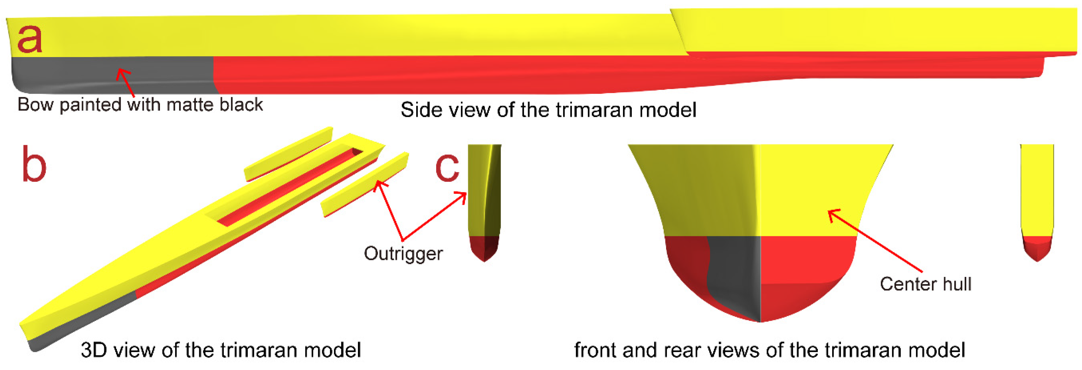
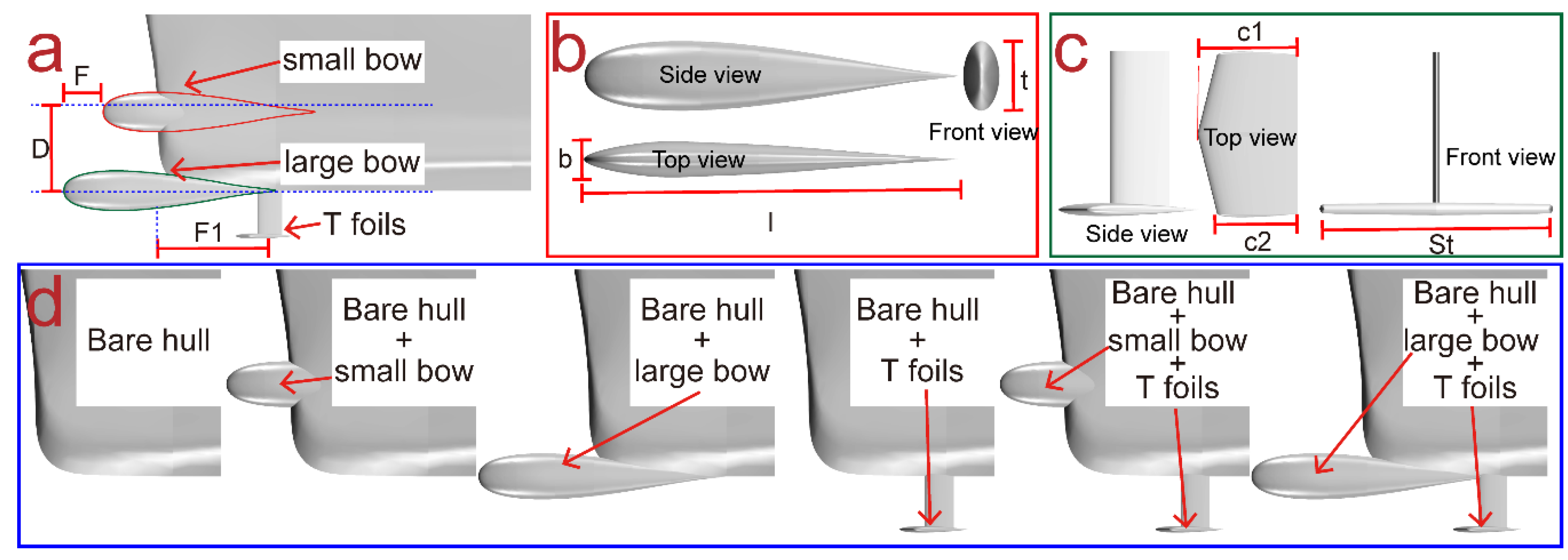
2. Geometric Model and Experimental Conditions
2.1. Experimental Modes
2.2. Experimental Conditions
3. Trim and Sinkage of the Hull with Different Appendages
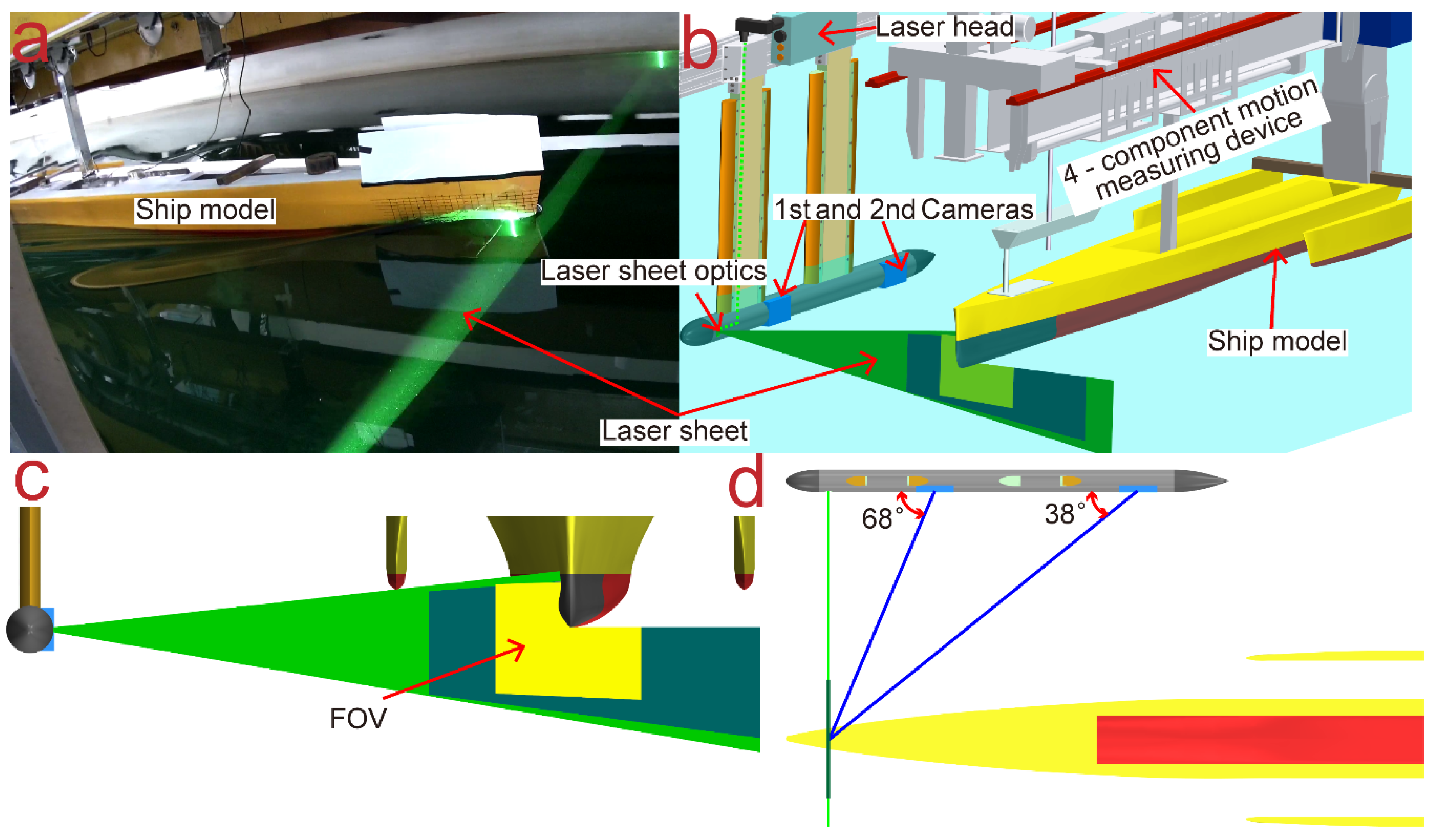
4. Experimental Setup
4.1. Facility and SPIV System
4.2. Test Details
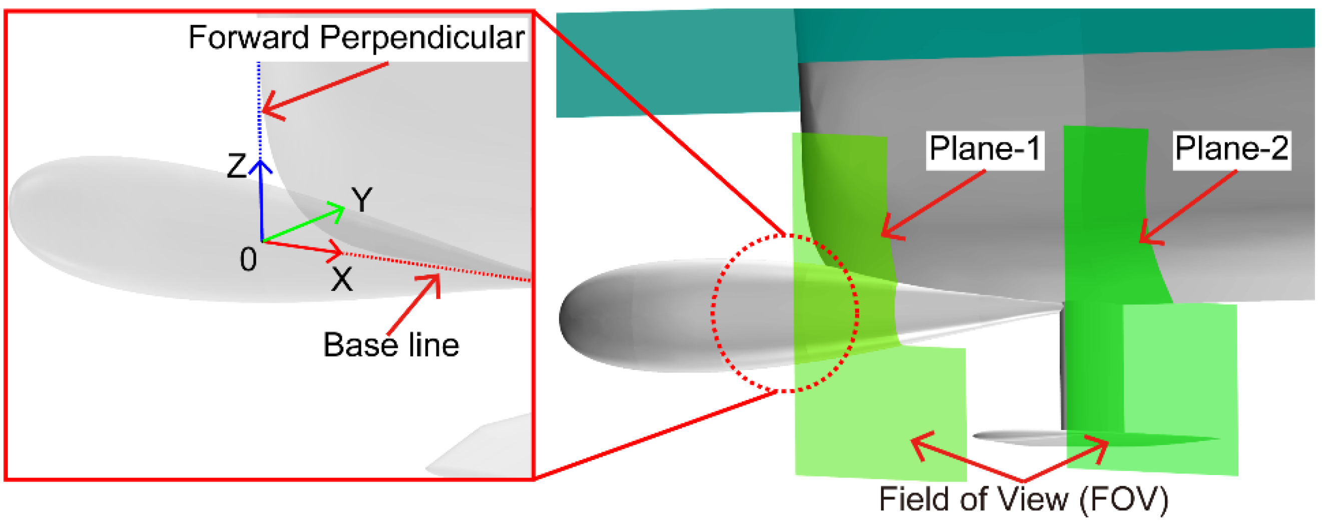
4.3. Analysis of the Velocity Field
5. Results and Discussion
5.1. Influence of a Bulbous Bow Type on the Axial Velocity Distribution
5.2. Influence of T Foils on the Axial Velocity Distribution
5.3. Influence of the Bow Wave on the Axial Velocity Distribution
6. Conclusions
- (1)
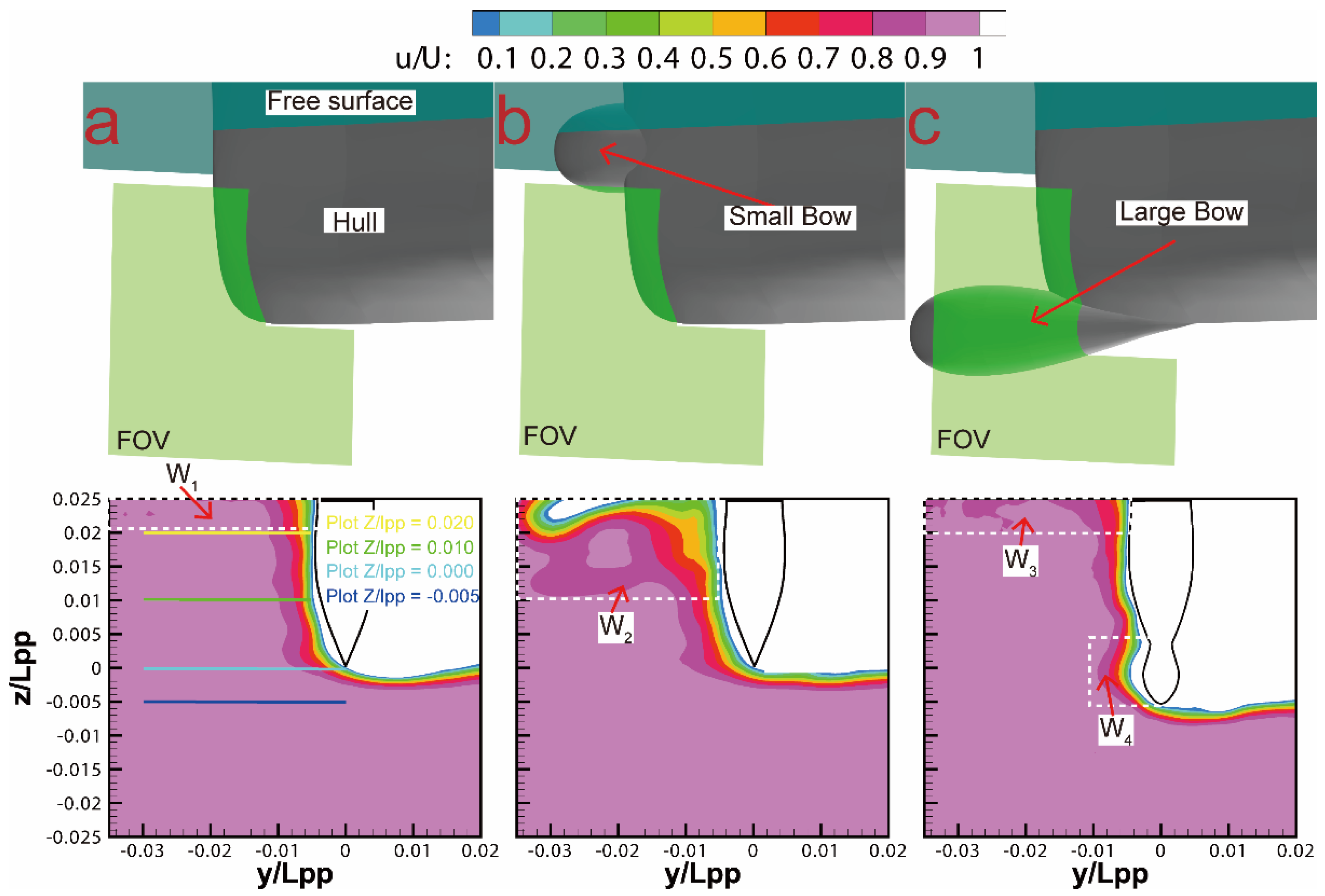
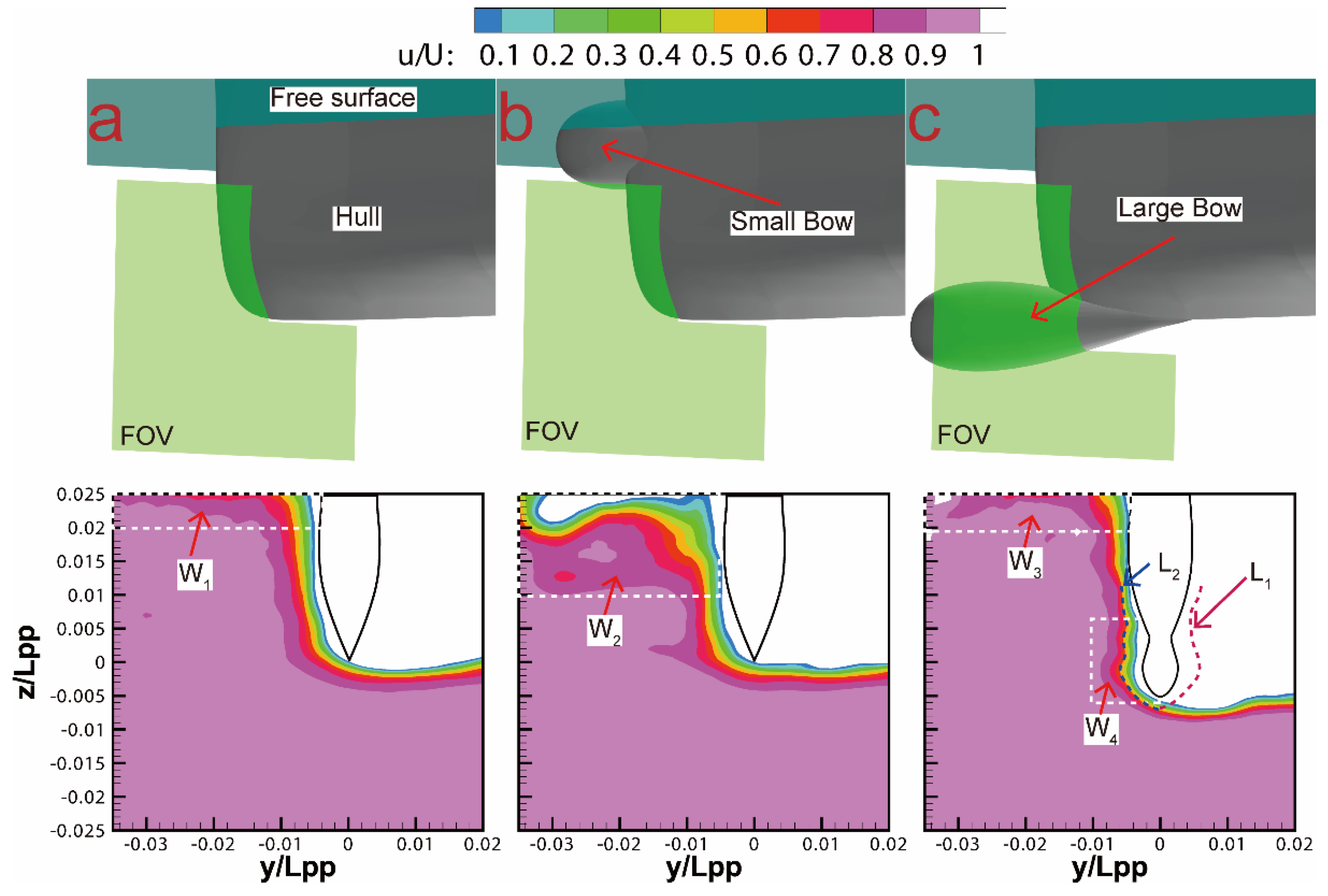
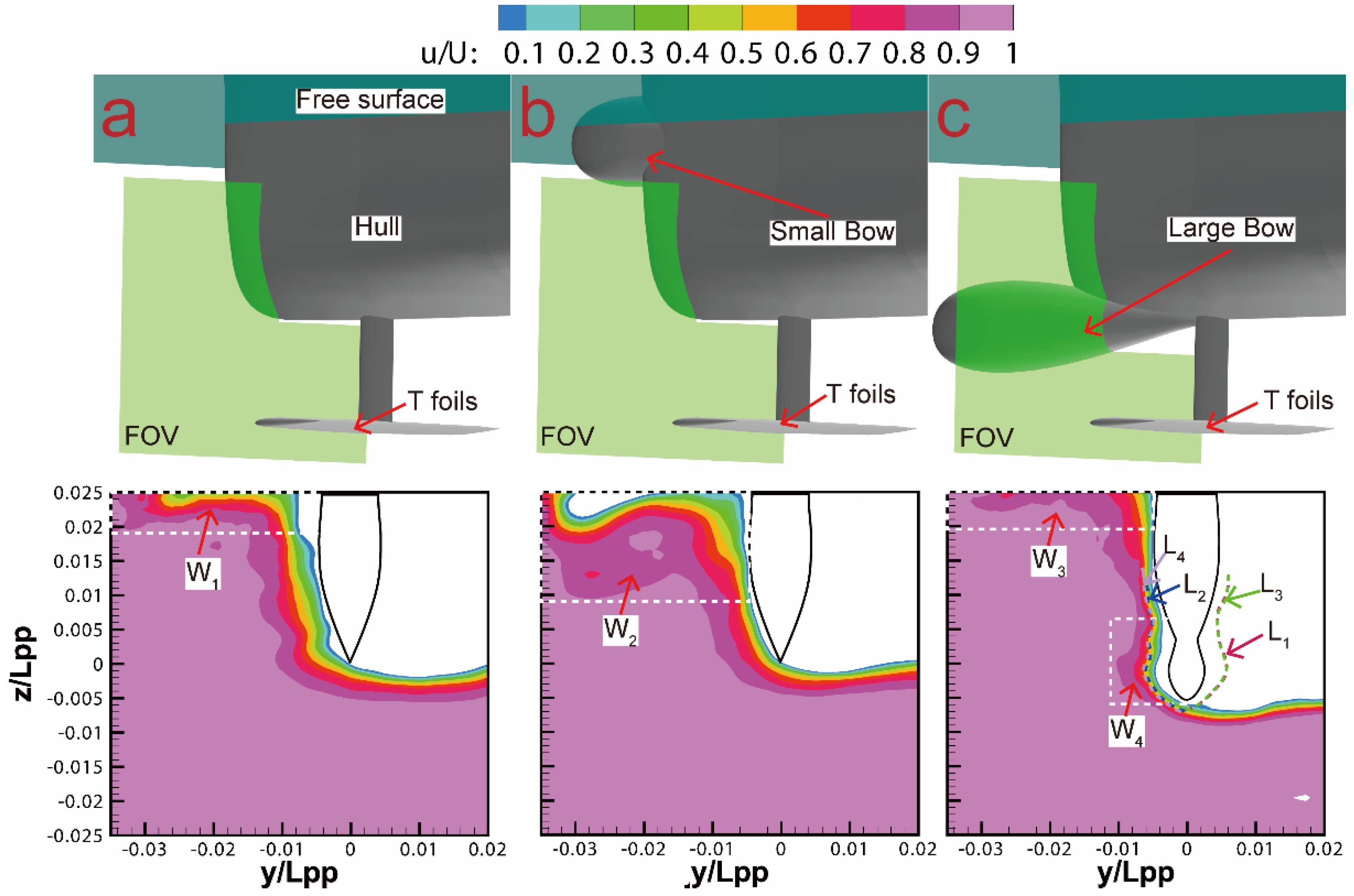
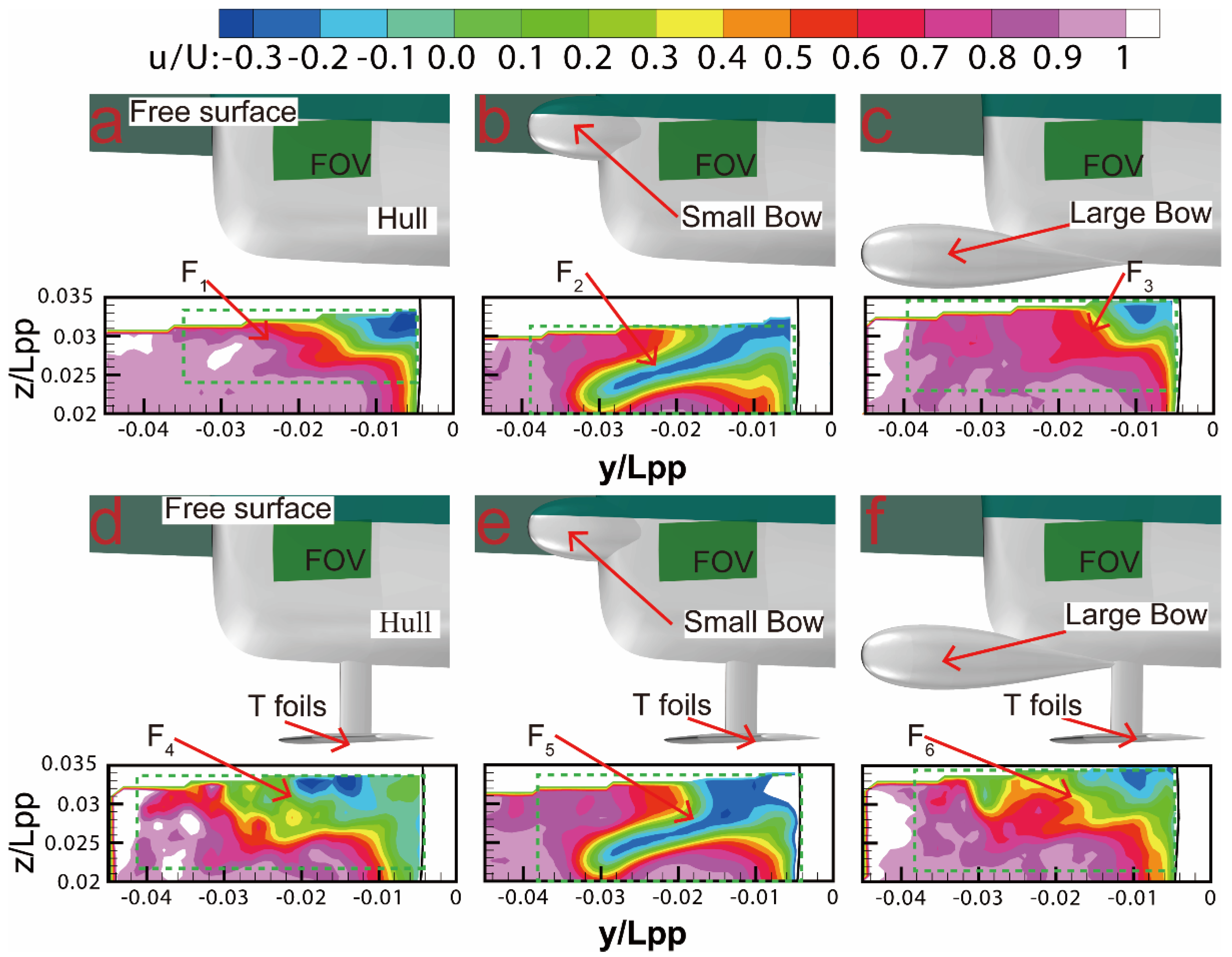
- The flow field distribution around the bulbous bow of a ship is mainly affected by the free surface, the horizontal and longitudinal curvature of the hull, and the hydrodynamic appendages installed in the bow. Since the midline of the small bulbous bow is in the free surface area, the interaction between the small bulbous bow and the free surface causes a disturbance of the water particles around the bow and a certain range of low-speed wake area is formed behind the small bulbous bow. In addition, the large bulbous bow has no effect on the distribution of the flow field around the free surface but mainly affects the distribution of the flow field around the bottom of the hull in the bow region.
- (2)
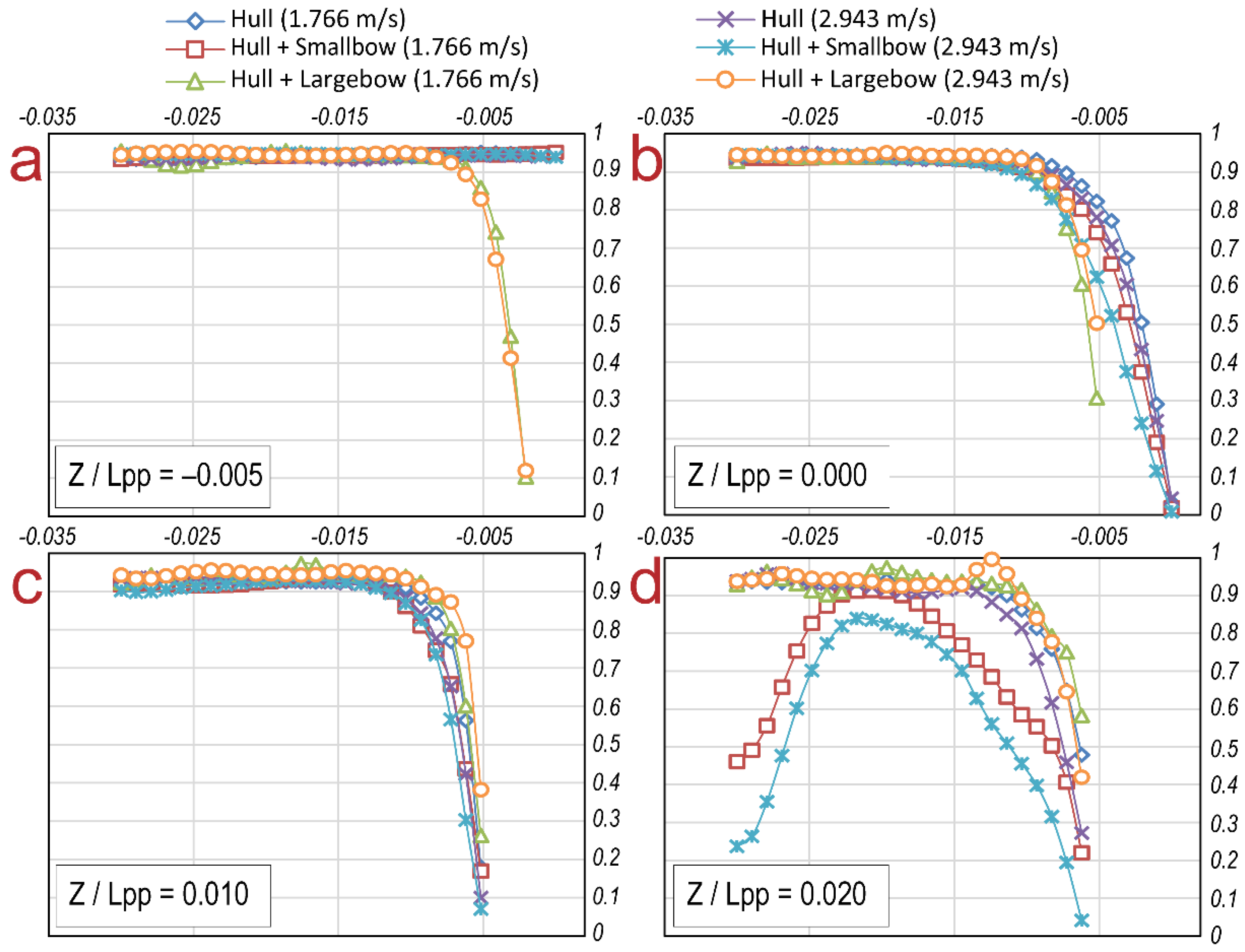
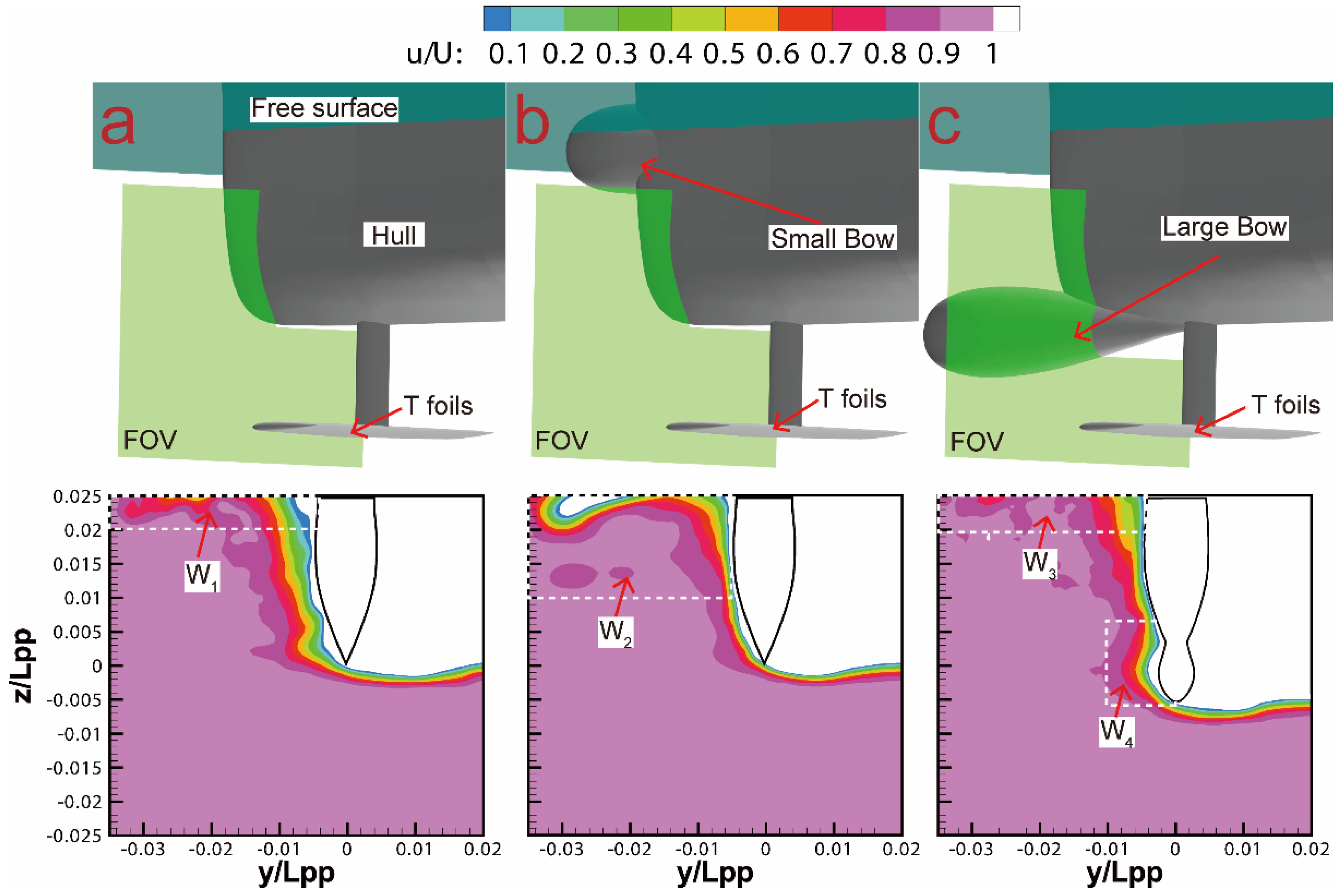
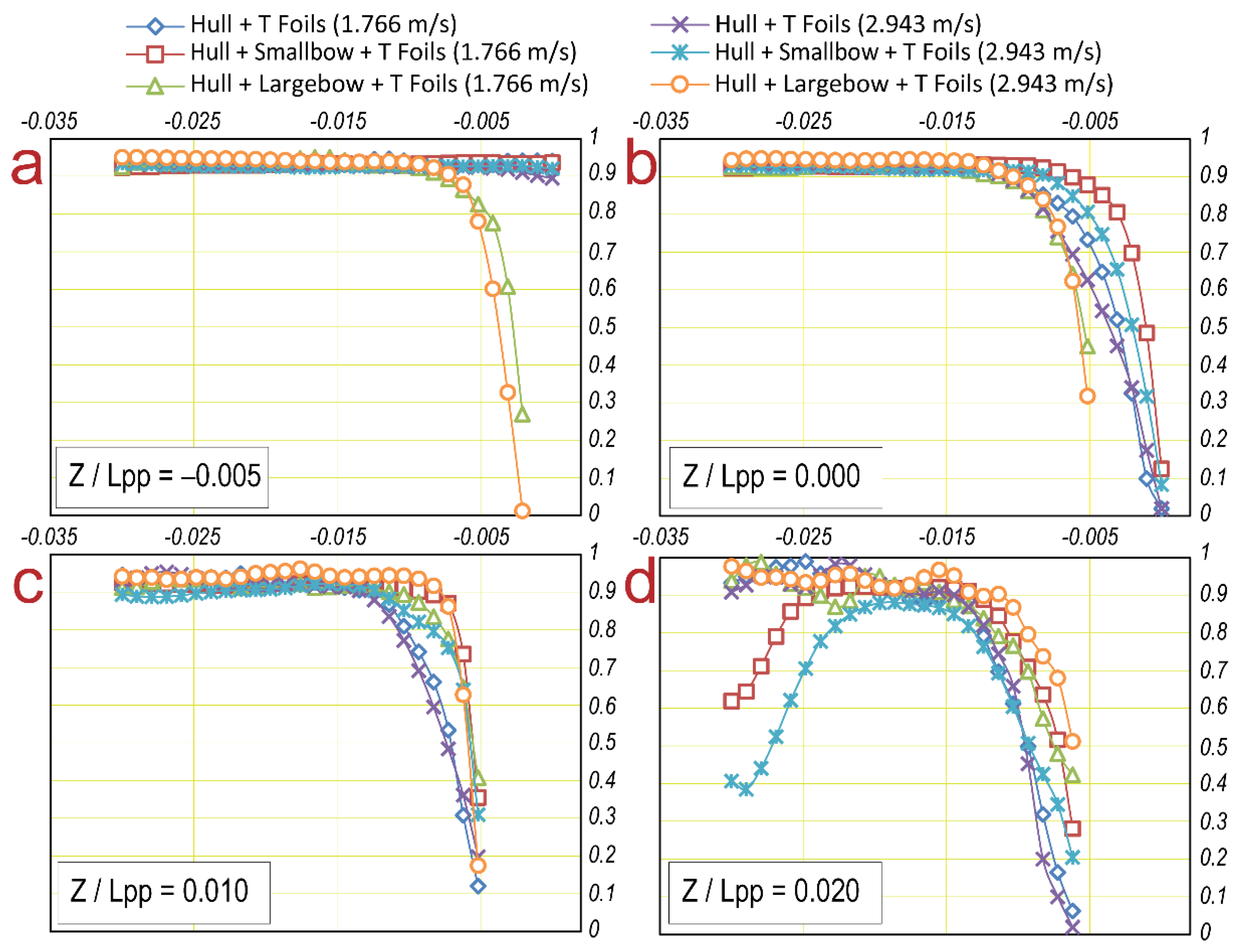
- Since T foils were installed at a distance behind test plane 1, the contribution of the T foils themselves to the disturbance of the flow field in test plane 1 could be considered negligible. T foils mainly affect the floating state of the ship in motion, such as sinkage and trim, during stable navigation, and a change in the floating state further affects the encounter state of the forward flow and the bow. Comparing Figure 5 and Figure 8, it can be seen that an increase in the local subsidence value increases the disturbance of the free surface by the ship’s bow. The difference in the flow field between the two working conditions is mainly manifested at the near free surface. Comparing Figure 6 and Figure 9, it can be seen that the ascent of test plane 1 reduces the disturbance of the free surface by the ship’s bow. The working condition with T foils installed, that is, the working condition with a smaller local positive heave value, has a larger range of disturbance of the flow field.
- (3)
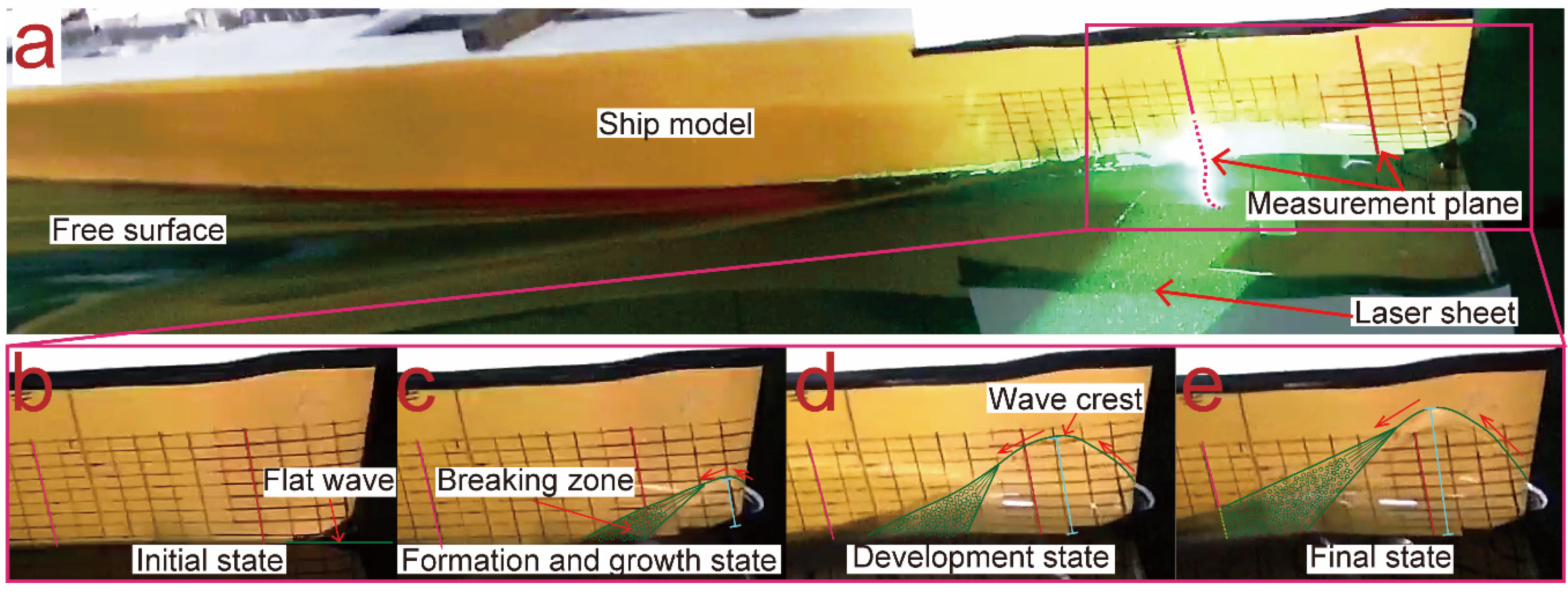
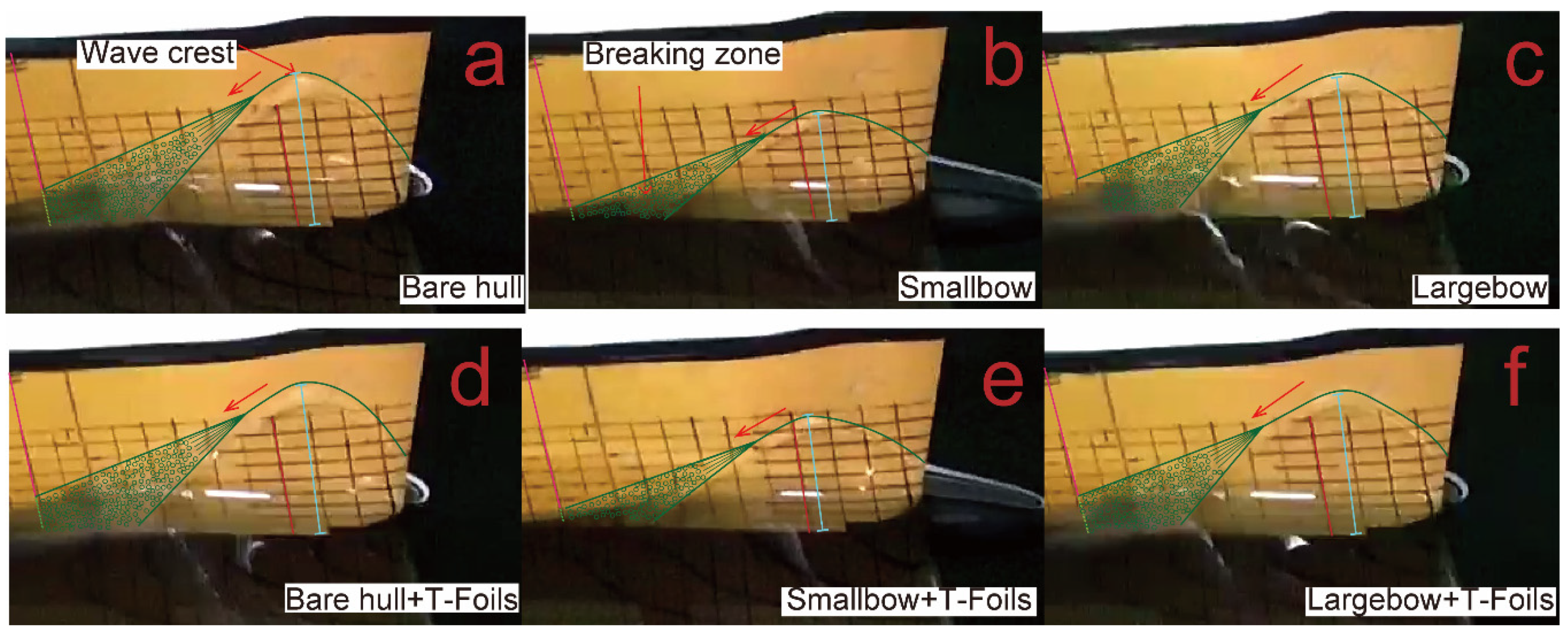
- The height and breaking range of the bow wave are important factors that affect the flow field around the bow in the near-free-surface area. The climbing of the water mass is accompanied by the breaking of the bow wave, and the breaking of the bow wave starts in the growth stage and gradually expands away from the bow during the development stage, reaching the maximum range in the stable stage. The order of the height and breaking range of the bow wave is as follows: bare hull with T foils > bare hull > bare hull with a large bow and T foils > bare hull with a large bow > bare hull with a small bow and T foils > bare hull with a small bow.
- (4)
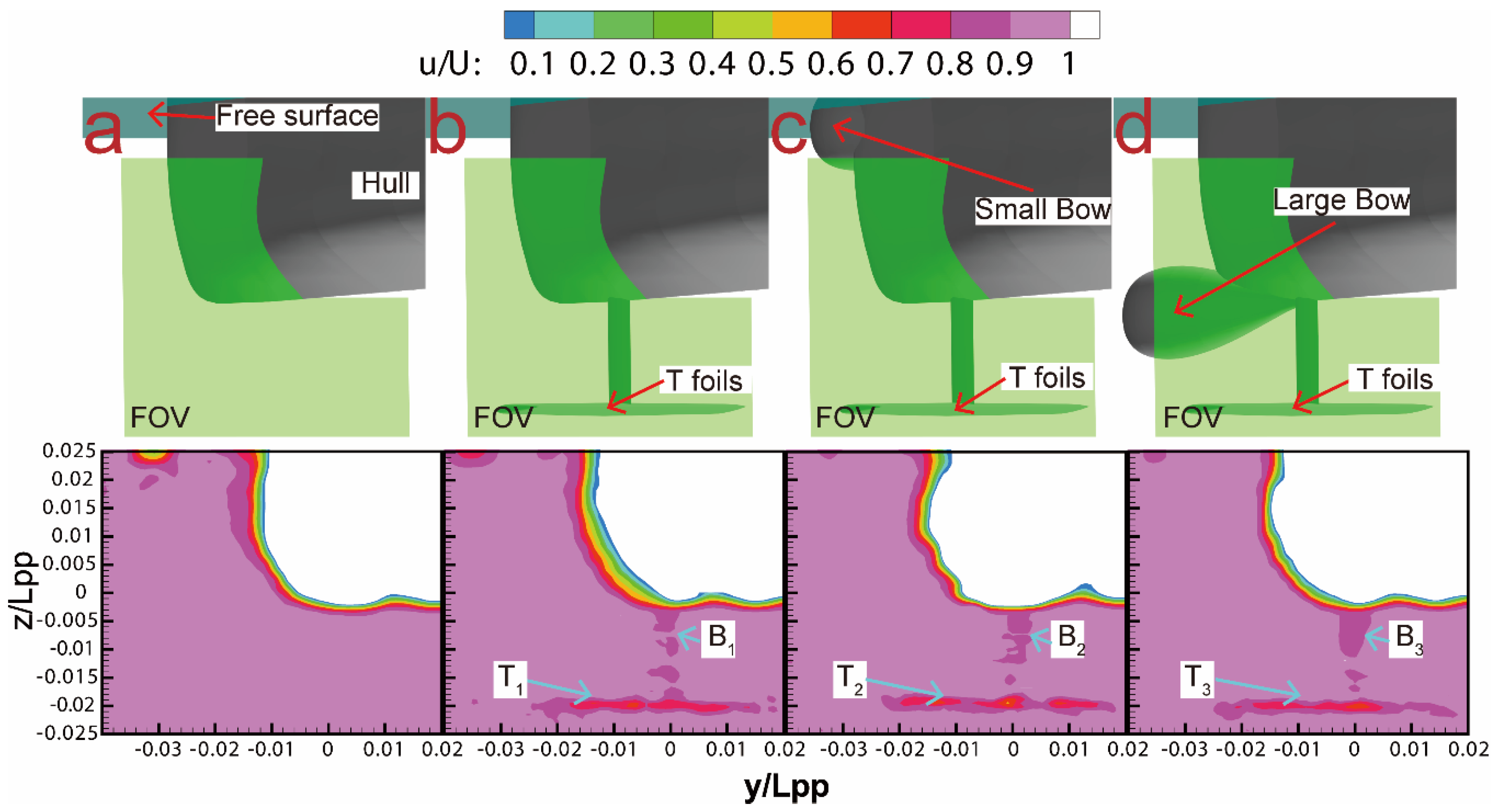
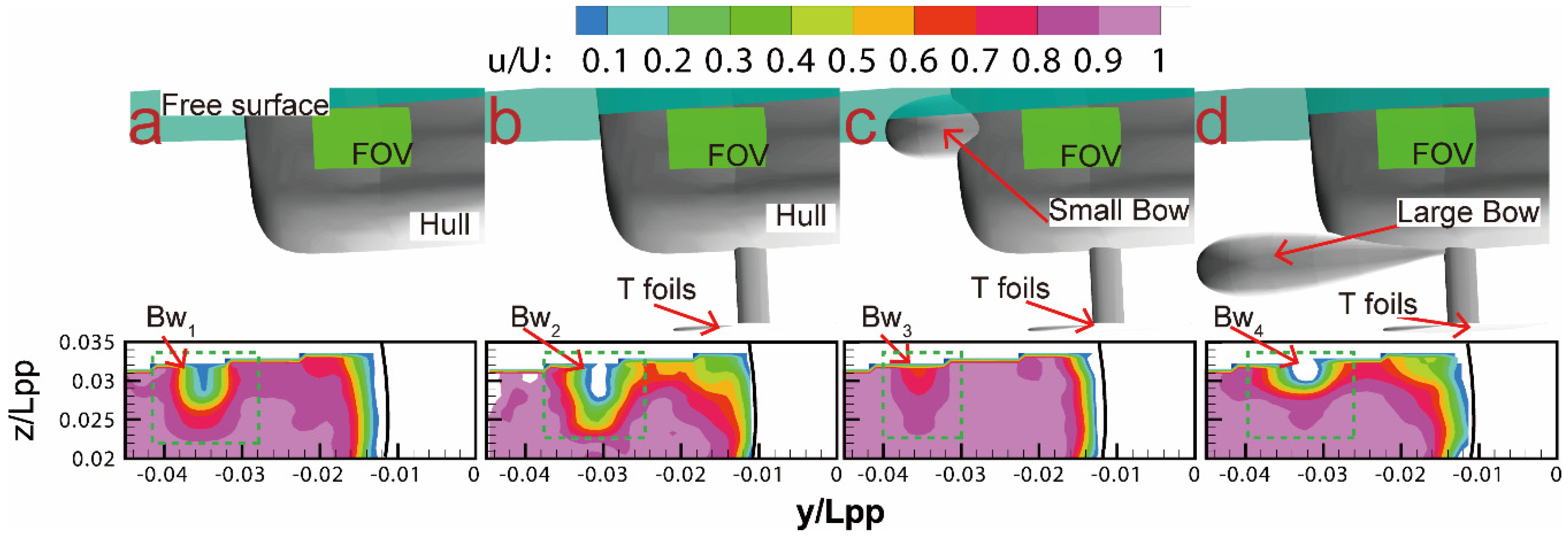
- The overall distribution of the flow field in test plane 1 of a bare hull, a bare hull with T foils, a bare hull with a large bow, and a bare hull with a large bow and T foils was similar. The difference is reflected in the range of flow field disturbance caused by the degree of bow wave action, and the range of the perturbed flow field near the free surface of a bare hull with T foils is the largest. For the testing conditions of a bare hull with a small bow and that with a small bow and T foils, the distribution of the flow field around the hull is quite different from that of other working conditions. This is because the flow field around the free surface area at this time is affected by the coupling effect of the wake field of the bulbous bow and the bow wave. The overall distribution and flow field disturbance range of the flow field in test plane 2 corresponded to the order of the height and breaking range of the bow wave in Figure 13.
Author Contributions
Funding
Institutional Review Board Statement
Informed Consent Statement
Data Availability Statement
Conflicts of Interest
References
- Dantec Dynamics. The World’s First Towing Tank PIV System. Available online: https://www.dantecdynamics.com/about/history/ (accessed on 20 July 2021).
- Gui, L.; Longo, J.; Stern, F. Biases of PIV measurement of turbulent flow and the masked correlation-based interrogation algorithm. Exp. Fluids 2001, 30, 27–35. [Google Scholar] [CrossRef]
- Gui, L.; Longo, J.; Stern, F. Towing Tank PIV Measurement System, Data and Uncertainty Assessment for DTMB Model 5512. Exp. Fluids 2001, 31, 336–346. [Google Scholar] [CrossRef]
- Di Felice, F.; Pereira, F. Developments and Applications of PIV in Naval Hydrodynamics. In Fluid Mechanics and Its Applications; Springer Science and Business Media LLC: New York, NY, USA, 2008; Volume 112, pp. 475–503. [Google Scholar]
- Yoon, H.S. Phase-Averaged Stereo-PIV Flow Field and Force/Moment/Motion Measurements for Surface Combatant in PMM Maneuvers. Ph.D. Thesis, Department of Mechanical Engineering, The University of Iowa, Iowa City, IA, USA, December 2009. [Google Scholar]
- ITTC. Available online: https://ittc.info/media/6087/sc-detailed-flow.pdf (accessed on 20 July 2021).
- ITTC. Available online: https://ittc.info/media/5540/15.pdf (accessed on 20 July 2021).
- ITTC. Available online: https://ittc.info/media/3491/volume2_4wakefield.pdf (accessed on 20 July 2021).
- Falchi, M.; Felli, M.; Grizzi, S.; Aloisio, G.; Broglia, R.; Stern, F. SPIV measurements around the DELFT 372 catamaran in steady drift. Exp. Fluids 2014, 55, 1844. [Google Scholar] [CrossRef]
- Yoon, H.; Longo, J.; Toda, Y.; Stern, F. Benchmark CFD validation data for surface combatant 5415 in PMM maneuvers—Part II: Phase-averaged stereoscopic PIV flow field measurements. Ocean Eng. 2015, 109, 735–750. [Google Scholar] [CrossRef] [Green Version]
- Guo, C.-Y.; Wu, T.-C.; Zhang, Q.; Gong, J. Numerical simulation and experimental research on wake field of ships under off-design conditions. Ocean Eng. 2016, 30, 821–834. [Google Scholar] [CrossRef]
- Guo, C.-Y.; Wu, T.-C.; Luo, W.-Z.; Chang, X.; Gong, J.; She, W.-X. Experimental study on the wake fields of a Panamax Bulker based on stereo particle image velocimetry. Ocean Eng. 2018, 165, 91–106. [Google Scholar] [CrossRef]
- Newman, J.N. Flow near the leading edge of a rectangular wing of small aspect ratio with applications to the bow of a ship. J. Eng. Math. 1973, 7, 163–172. [Google Scholar] [CrossRef]
- Hirata, M.H. The flow near the bow of a steadily turning ship. J. Fluid Mech. 1975, 71, 283–291. [Google Scholar] [CrossRef]
- Oertel, R. The steady motion of a flat ship including an investigation of local flow near the bow. Bull. Aust. Math. Soc. 1976, 14, 315–316. [Google Scholar] [CrossRef] [Green Version]
- Grosenbaugh, M.A.; Yeung, R.W. Flow Structure Near a Ship Bow: An Experimental Investigation; NAOE-85-1; Department of Naval Architecture and Ocean Engineering, University of California: Berkeley, CA, USA, 1985. [Google Scholar]
- Grosenbaugh, M.A.; Yeung, R.W. Flow Structure Near the Bow of a Two-Dimensional Body. J. Ship Res. 1989, 33, 269–283. [Google Scholar] [CrossRef]
- Fry, D.J.; Kim, Y.H. Bow Flow of Surface Ships. In Proceedings of the 15th Symposium on Naval Hydrodynamics, Hamburg, Germany, 2 June 1985; pp. 319–346. [Google Scholar]
- Maruo, H.; Ikehata, M. Some discussions on the free-surface flow around the bow. In Proceedings of the 16th Symposium on Naval Hydrodynamics, Berkeley, CA, USA, 13–18 July 1986; pp. 65–77. [Google Scholar]
- Longo, J.; Stern, F.; Toda, Y. Mean-Flow Measurements in the Boundary Layer and Wake and Wave Field of a Series 60 CB = 0.6 Ship Model—Part 2: Scale Effects on Near-Field Wave Patterns and Comparisons with Inviscid Theory. J. Ship Res. 1993, 37, 16–24. [Google Scholar] [CrossRef]
- Toda, Y.; Stern, F.; Longo, J. Mean-Flow Measurements in the Boundary Layer and Wake and Wave Field of a Series 60 CB = 0.6 Ship Model—Part 1: Froude Numbers 0.16 and 0.316. J. Ship Res. 1992, 36, 360–377. [Google Scholar] [CrossRef]
- Toda, Y.; Stern, F.; Takana, V.; Patel, V.C. Mean-Flow Measurements in the Boundary Layer and Wake of a Series 60 CB = 0.6 Model Ship with and without Propeller. J Ship Res. 1990, 34, 225–252. [Google Scholar] [CrossRef]
- Stern, F.; Longo, J.; Zhang, Z.J.; Subramani, A.K. Detailed Bow-Flow Data and CFD for a Series 60 CB = 0.6 Ship Model for Froude Number 0.316. J. Ship Res. 1996, 40, 193–199. [Google Scholar] [CrossRef]
- Longo, J.; Stern, F. Effects of drift angle on model ship flow. Exp. Fluids 2002, 32, 558–569. [Google Scholar] [CrossRef]
- Tahara, Y.; Longo, J.; Stern, F. Comparison of CFD and EFD for the Series 60 CB = 0.6 in steady drift motion. J. Mar. Sci. Technol. 2002, 7, 17–30. [Google Scholar] [CrossRef]
- Dong, R.R.; Katz, J.; Huang, T.T. On the structure of bow waves on a ship model. J. Fluid Mech. 1997, 346, 77–115. [Google Scholar] [CrossRef]
- Roth, G.I.; Mascenik, D.T.; Katz, J. Measurements of the flow structure and turbulence within a ship bow wave. Phys. Fluids 1999, 11, 3512–3523. [Google Scholar] [CrossRef]
- Mallat, B.; Germain, G.; Delacroix, S.; Druault, P. PIV measurements around a bow ship. In Proceedings of the Workshop on Non-Intrusive Measurements for Unsteady Flows and Aerodynamics, Poitiers, France, 27–29 October 2005. [Google Scholar]
- Mallat, B.; Germain, G.; Gaurier, B.; Druault, P. Study of the Bubble Sweep-down Phenomenon on Two Ship Models. In Proceedings of the 31th Symposium on Naval Hydrodynamics, Monterey, CA, USA, 11–26 September 2016. [Google Scholar]
- Cozijn, J.L.; Hallmann, R. Thruster-Interaction Effects on a DP Shuttle Tanker-Wake Flow Measurements of the Main Propeller and Bow Tunnel Thrusters. In Proceedings of the 33rd International Conference on Ocean, Offshore and Arctic Engineering, San Francisco, CA, USA, 1 June 2014. [Google Scholar]
- Yoon, H.; Gui, L.; Bhushan, S.; Stern, F. Tomographic PIV Measurements For Surface Combatant 5415 Straight Ahead and Static Drift 10 and 20 Degree Conditions. In Proceedings of the 30th Symposium on Naval Hydrodynamics, Hobart, TAS, Australia, 2–7 November 2014. [Google Scholar]
- Bhushan, S.; Yoon, H.; Stern, F.; Guilmiuau, E.; Visonneau, M.; Toxopeus, S.; Simonsen, C.; Aram, S.; Kim, S.E.; Griporopoulos, G.; et al. CFD Validation for Surface Combatant 5415 Straight Ahead and Static Drift 20 Degree Conditions. Presented at the SNAME 5th World Maritime Technology Conference, Providence, RI, USA, 3–7 November 2015. [Google Scholar]
- Bhushan, S.; Yoon, H.; Stern, F. Large grid simulations of surface combatant flow at straight-ahead and static drift conditions. Int. J. Comput. Fluid Dyn. 2016, 30, 356–362. [Google Scholar] [CrossRef]
- Jacobi, G.; Thill, C.H.; Huijsmans, R.H.M. Pressure reconstruction from velocity field measurements obtained with particle image velocimetry in the bow region of a fast ship. In Proceedings of the 6th International Conference on Advanced Model Measurement Technology for The Maritime Industry AMT’19, Rome, Italy, 9–11 October 2019. [Google Scholar]
- Deng, R.; Luo, F.; Wu, T.; Chen, S.; Li, Y. Time-domain numerical research of the hydrodynamic characteristics of a trimaran in calm water and regular waves. Ocean Eng. 2019, 194, 106669. [Google Scholar] [CrossRef]
- Kandasamy, M.; Wu, P.C.; Zalek, S.; Karr, D.; Bartlett, S.; Nguyen, L. CFD based Hydrodynamic Optimization and Structural Analysis of the Hybrid Ship Hull. In Proceedings of the SNAME Annual Meeting and Expo and Ship Production Symposium, Houston, TX, USA, 22–24 October 2014. [Google Scholar]
- Peltzer, T.J.; Keipper, T.S.; Kays, B.; Shimozono, G. A New Paradigm for High-Speed Monohulls: The Bow Lifting Body Ship. Available online: https://citeseerx.ist.psu.edu/viewdoc/download?doi=10.1.1.482.7035&rep=rep1&type=pdf (accessed on 20 July 2021).
- Zong, Z.; Sun, Y.; Jiang, Y. Experimental study of controlled T-foil for vertical acceleration reduction of a trimaran. J. Mar. Sci. Technol. 2018, 24, 553–564. [Google Scholar] [CrossRef]
- Luo, W.; Guo, C.; Wu, T.; Xu, P.; Su, Y. Experimental study on the wake fields of a ship attached with model ice based on stereo particle image velocimetry. Ocean Eng. 2018, 164, 661–671. [Google Scholar]
- Wu, T.; Luo, W.; Jiang, D.; Deng, R.; Li, Y. Stereo Particle Image Velocimetry Measurements of the Wake Fields Behind A Panamax Bulker Ship Model Under the Ballast Condition. J. Mar. Sci. Eng. 2020, 8, 397. [Google Scholar] [CrossRef]
- Wu, T.C.; Deng, R.; Luo, W.Z.; Sun, P.N.; Dai, S.S.; Li, Y.L. 3D-3C wake field measurement, reconstruction and spatial distribution of a Panamax Bulk using towed underwater 2D–3C SPIV. Appl. Ocean Res. 2020, 105, 102437. [Google Scholar] [CrossRef]
- Bendat, J.S.; Piersol, A.G. Random Data—Analysis and Measurement Procedures, 2nd ed.; John Wiley & Sons, Inc.: Hoboken, NJ, USA, 1986. [Google Scholar]
- Bendat, J.S.; Piersol, A.G. Random Data—Analysis and Measurement Procedures, 4th ed.; John Wiley & Sons, Inc.: Hoboken, NJ, USA, 2010. [Google Scholar]
- Dong, M.S.; Jeong, H.S.; Shin, H.R. Towed underwater PIV measurement for free-surface effects on turbulent wake of a surface-piercing body. Int. J. Nav. Archit. 2013, 5, 404–413. [Google Scholar]


| Principal Hull Data | Center Hull | Outrigger | |
|---|---|---|---|
| Length between perpendiculars (m) | Lpp | 3.60 | 1.25 |
| Breadth (m) | B | 0.28 | 0.05 |
| Draft (m) | T | 0.13 | 0.04 |
| Displacement (kg) | ∆ | 73.10 | 1.05 |
| Wet surface area (m2) | S | 0.84 | 0.05 |
| Testing Conditions | Unit | Parameters |
|---|---|---|
| Test plane-1 | - | X/Lpp = 0.0167 |
| Test plane-2 | - | X/Lpp = 0.0611 |
| Draft of center hull | m | 0.13 |
| Draft of outrigger | m | 0.04 |
| Fluid medium | - | Water |
| Test speed | m/s | 1.766, 2.943 |
| Wave conditions | - | Clam water |
| Testing Model | Sinkage (mm) | Trim (°) | ||
|---|---|---|---|---|
| 1.766 m/s | 2.943 m/s | 1.766 m/s | 2.943 m/s | |
| Bare hull | −3.761 | −13.360 | 0.008 | 0.544 |
| Bare hull with a small bulbous bow | −3.840 | −13.160 | 0.013 | 0.559 |
| Bare hull with a large bulbous bow | −3.680 | −13.160 | 0.006 | 0.498 |
| Bare hull with T foils | −4.077 | −13.724 | −0.020 | 0.483 |
| Bare hull with a small bulbous bow and T foils | −4.149 | −13.665 | −0.017 | 0.519 |
| Bare hull with a large bulbous bow and T foils | −4.180 | −13.739 | −0.008 | 0.431 |
| Testing Model | 1.766 m/s | 2.943 m/s | ||||
|---|---|---|---|---|---|---|
| ∆Zsinkage (mm) | ∆Ztrim (mm) | Zplane-1 (mm) | ∆Zsinkage (mm) | ∆Ztrim (mm) | Zplane-1 (mm) | |
| Bare hull | −3.761 | 0.243 | −3.518 | −13.360 | 16.512 | 3.152 |
| Bare hull with a small bulbous bow | −3.840 | 0.395 | −3.445 | −13.160 | 16.967 | 3.807 |
| Bare hull with a large bulbous bow | −3.680 | 0.182 | −3.498 | −13.160 | 15.115 | 1.955 |
| Bare hull with T foils | −4.077 | −0.607 | −4.684 | −13.724 | 14.660 | 0.936 |
| Bare hull with a small bulbous bow and T foils | −4.149 | −0.516 | −4.665 | −13.665 | 15.753 | 2.088 |
| Bare hull with a large bulbous bow and T foils | −4.180 | −0.243 | −4.423 | −13.739 | 13.082 | −0.657 |
| Testing Model | 1.766 m/s | ||
|---|---|---|---|
| ∆Zsinkage (mm) | ∆Ztrim (mm) | Zplane-2 (mm) | |
| Bare hull | −3.761 | 0.221 | −3.540 |
| Bare hull with T foils | −4.077 | −0.551 | −4.628 |
| Bare hull with a small bulbous bow and T foils | −4.149 | −0.469 | −4.618 |
| Bare hull with a large bulbous bow and T foils | −4.180 | −0.221 | −4.401 |
Publisher’s Note: MDPI stays neutral with regard to jurisdictional claims in published maps and institutional affiliations. |
© 2021 by the authors. Licensee MDPI, Basel, Switzerland. This article is an open access article distributed under the terms and conditions of the Creative Commons Attribution (CC BY) license (https://creativecommons.org/licenses/by/4.0/).
Share and Cite
Deng, R.; Wang, S.; Luo, W.; Wu, T. Experimental Study on the Influence of Bulbous Bow Form on the Velocity Field around the Bow of a Trimaran Using Towed Underwater 2D-3C SPIV. J. Mar. Sci. Eng. 2021, 9, 905. https://doi.org/10.3390/jmse9080905
Deng R, Wang S, Luo W, Wu T. Experimental Study on the Influence of Bulbous Bow Form on the Velocity Field around the Bow of a Trimaran Using Towed Underwater 2D-3C SPIV. Journal of Marine Science and Engineering. 2021; 9(8):905. https://doi.org/10.3390/jmse9080905
Chicago/Turabian StyleDeng, Rui, Shigang Wang, Wanzhen Luo, and Tiecheng Wu. 2021. "Experimental Study on the Influence of Bulbous Bow Form on the Velocity Field around the Bow of a Trimaran Using Towed Underwater 2D-3C SPIV" Journal of Marine Science and Engineering 9, no. 8: 905. https://doi.org/10.3390/jmse9080905