A Spectral Method for Two-Dimensional Ocean Acoustic Propagation

Abstract

The accurate calculation of the sound field is one of the most concerning issues in hydroacoustics. The one-dimensional spectral method has been used to correctly solve simplified underwater acoustic propagation models, but it is difficult to solve actual ocean acoustic fields using this model due to its application conditions and approximation error. Therefore, it is necessary to develop a direct solution method for the two-dimensional Helmholtz equation of ocean acoustic propagation without using simplified models. Here, two commonly used spectral methods, Chebyshev–Galerkin and Chebyshev–collocation, are used to correctly solve the two-dimensional Helmholtz model equation. Since Chebyshev–collocation does not require harsh boundary conditions for the equation, it is then used to solve ocean acoustic propagation. The numerical calculation results are compared with analytical solutions to verify the correctness of the method. Compared with the mature Kraken program, the Chebyshev–collocation method exhibits higher numerical calculation accuracy. Therefore, the Chebyshev–collocation method can be used to directly solve the representative two-dimensional ocean acoustic propagation equation. Because there are no model constraints, the Chebyshev–collocation method has a wide range of applications and provides results with high accuracy, which is of great significance in the calculation of realistic ocean sound fields.

1. Introduction

In recent years, underwater acoustic technology has been widely used to detect underwater targets [1], describe underwater overviews [2], measure hydrological information [3], and perform other tasks [4]. Due to the influence of the water surface, water body, water bottom, and other features, sound wave propagation in the ocean presents a complicated distribution state [5]. According to the principle of ocean acoustic propagation, sound waves of a fixed frequency satisfy the elliptic partial differential Helmholtz equation. The sound pressure results throughout an entire space can be obtained after adding boundary conditions to constrain the Helmholtz equation [6]. Recently, Wang et al. [7] used the one-dimensional spectral method to correctly solve the parabolic equation model. Due to the high accuracy and fast convergence speed of the spectral method, it has greatly promoted the development of ocean acoustic calculation. However, there are still some problems in the process of calculation. For example, the beginning of this calculation method solves the simplified parabolic model of the Helmholtz equation. Although simplified models make numerical solutions easier to obtain, their scope of application is very narrow, and approximation errors are introduced. For example, the parabolic equation model replaces the elliptic equation with the parabolic equation. It is thus suitable only for situations in which the physical parameters change slowly with the horizontal distance and the far-field assumption is adopted [8,9,10,11]. The contribution of the reverse acoustic wave to the full-field wave is ignored, and only the one-way acoustic propagation problem can be solved [8]. The normal mode model is appropriate only for cases in which the physical parameters are constant, and this model cannot be used to solve problems in which these quantities change with distance, as in actual ocean environments [12]. The ray model can be applied to high-frequency situations, that is, when the wavelength of the sound wave is significantly smaller than any physical scale in the problems [6]. The mirror image method uses the superposition of the real sound source point and the mirrored sound source point to obtain the real sound field, but its requirements for sound speed are more stringent; thus, this method can only be used to determine ocean sound fields with a constant sound speed profile [13]. The wavenumber integration method is suitable only for horizontally layered media and uses numerical integration to determine the sound field [13]. As a result, the calculated sound does not reflect the real marine environment if the sea area does not meet the constraints of the applied simplified model. Most actual marine environments are relatively complex, and relatively few meet the constraints of various models. Therefore, it is necessary to develop a direct solution to the two-dimensional Helmholtz equation of acoustic propagation without using simplified models.

It is usually difficult to directly solve the partial differential Helmholtz equation’s analytical solution. The finite difference method, finite element method and spectral method are commonly used discrete numerical methods for solving differential equations [14]. Among them, the finite difference and finite element methods are local approximation methods, and the spectral method is a global approximation method. The finite difference method is the most mature numerical method [15] and uses the difference quotient instead of the derivative. Its theoretical background and calculation are simple, and its format and structure are flexible. In 2007, a nine-point sixth-order accurate compact finite-difference method for solving the Helmholtz equation was developed and analyzed, but it can only solve the equation with the Neumann boundary condition [16]. In 2019, Zhu and Zhao proposed a high-order fast algorithm for solving the two-dimensional Helmholtz equation with Dirichlet and Neumann boundary conditions in polar coordinates [17]. Because the finite difference method has difficulty dealing with the Helmholtz equation with complex boundary conditions, it is commonly used to deal with the simplified partial differential equation of the Helmholtz equation for ocean acoustic propagation. At present, some mature ocean acoustic calculation programs have been developed using the finite difference method, such as RAM [18] based on the parabolic equation model and Kraken [19] based on the normal mode model. However, the finite difference method is not flexible enough to address complex boundary value problems in actual applications, and its approximation accuracy is limited by the format itself. Moreover, it is prone to instability. The finite element method decomposes a continuous area into a finite number of interconnected elements that can be polygons or other geometric shapes. This method easily addresses complex problems, but the accuracy of the approximation is also limited by the format itself [20]. Among the three commonly used numerical methods, the finite difference method and finite element method are both low-precision methods. With continued development of and improvement through scientific research, the study of small-scale and delicate problems has become increasingly important, and high-precision numerical methods have become a research focus of many scholars. The spectral method theoretically has infinite-order approximation accuracy and exponential-order convergence [21], and the spectral method can obtain high-precision results with a small degree of freedom, unlike the results of the finite difference method and the finite element method.

The classical numerical discrete methods are derived from the weighted residual method (MWR). The MWR linearly expands the solution under a set of trial functions, selects a set of test functions and approximate solutions as inner products, and finally forces the residual to zero. The spectral method is different from other numerical calculation methods, mainly in the selection of a class of globally smooth function clusters as trial functions and test functions. Commonly used function clusters include Chebyshev polynomials [22], Legendre polynomials [23], and Fourier functions [24]. The test function clusters are mainly divided into Galerkin, Tau and collocation types. Among them, the Galerkin and Tau types require that the trial function and test function are exactly the same, and the collocation type requires that the boundary conditions are met at the preselected grid points (i.e., collocation points). The name of each spectral method is described as an “A–B” type, where A is the type of trial function, such as Chebyshev, Legendre or Fourier, and B is the classification of the test function, such as Galerkin or collocation. Commonly used spectral methods include the Chebyshev–Galerkin spectral method and Chebyshev–collocation spectral method. In the 1980s, studies by Quartreroni, Canuto, Guo Benyu and others showed that the spectral method has infinite-order convergence, and the spectral method was applied to solve partial differential equations. Since then, the spectral method has been widely used to solve mathematical and physical problems [25,26,27,28,29,30]. The spectral method also has obvious advantages in solving atmospheric circulation problems [31]. In terms of the numerical eddy flow problem, the spectral method can be used to calculate the fluid flow in a straight channel, and the calculated laminar flow and turbulent flow results are in good agreement with the theoretical results [32]. The step-by-step pseudospectral method is used in the calculation of the water wave motion problem, and the pseudospectral method is established to numerically solve the two-dimensional tidal wave equation calculation model. As a result, the water wave motion caused by the perturbation of the water column of a uniform square pool is simulated and calculated [33]. In recent years, some scholars have begun to apply the spectral method to acoustic problems. Wise et al. [34] used the Fourier–collocation method to re-express the distribution of arbitrary sound sources and sensors, Wang et al. [35] proposed an improved sound propagation operator expansion scheme based on the spectral method, and Lan et al. [36] introduced an algorithm based on the spectral collocation method and were the first to explained the basic governing equations. In the calculation of ocean acoustics, Evans et al. [37] proposed a Legendre–Galerkin spectral method to solve the differential eigenvalue problem of complex and discontinuous coefficients in ocean acoustics.

In recent years, many scholars have studied direct solutions of two-dimensional partial differential equations using the spectral method. In 1995, Shen [38] used the Chebyshev–Galerkin spectral method to directly solve the two-dimensional Helmholtz equation with Dirichlet and Neumann boundary conditions, which achieved good results. In 2009, Wang et al. [39] used the Chebyshev-Tau and Chebyshev–Galerkin spectral methods to solve the two-dimensional Poisson equation. In 2019, Sahuck [40] successfully used the Chebyshev–Galerkin spectral method and quasi-inverse technique to directly solve the two-dimensional Poisson equation and Helmholtz equation with Dirichlet boundary conditions.

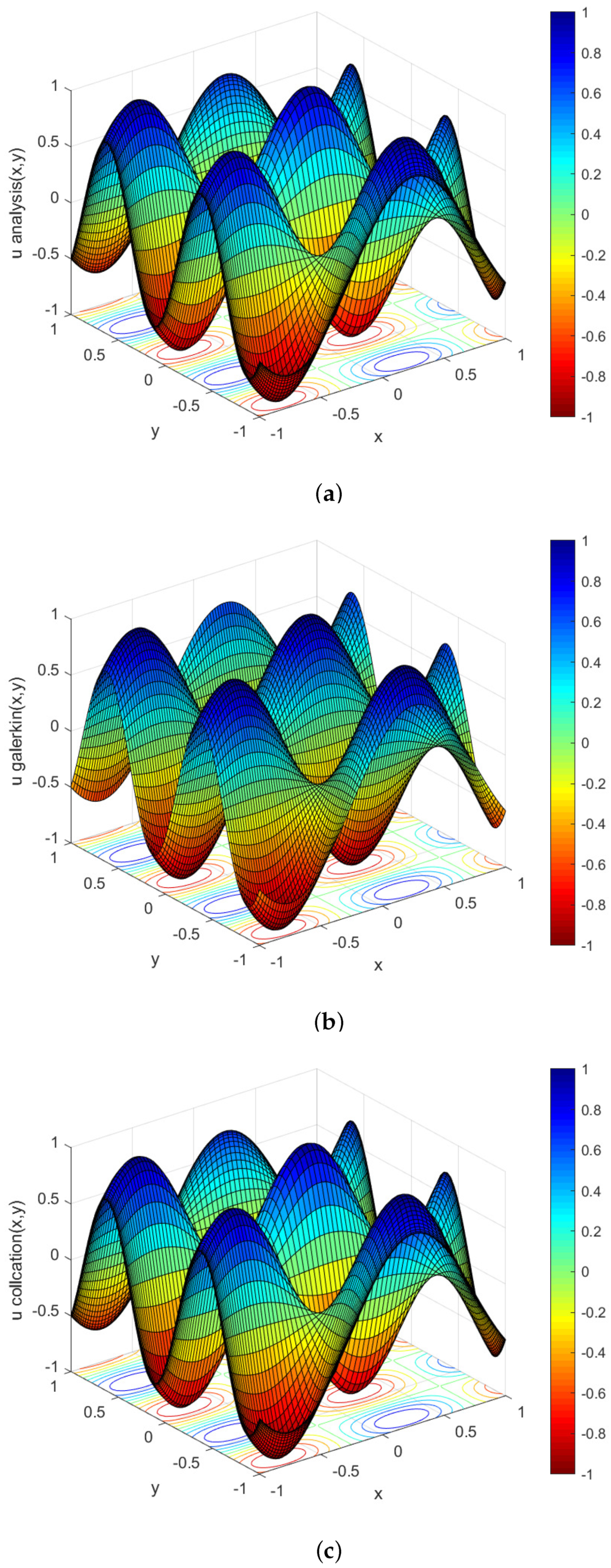
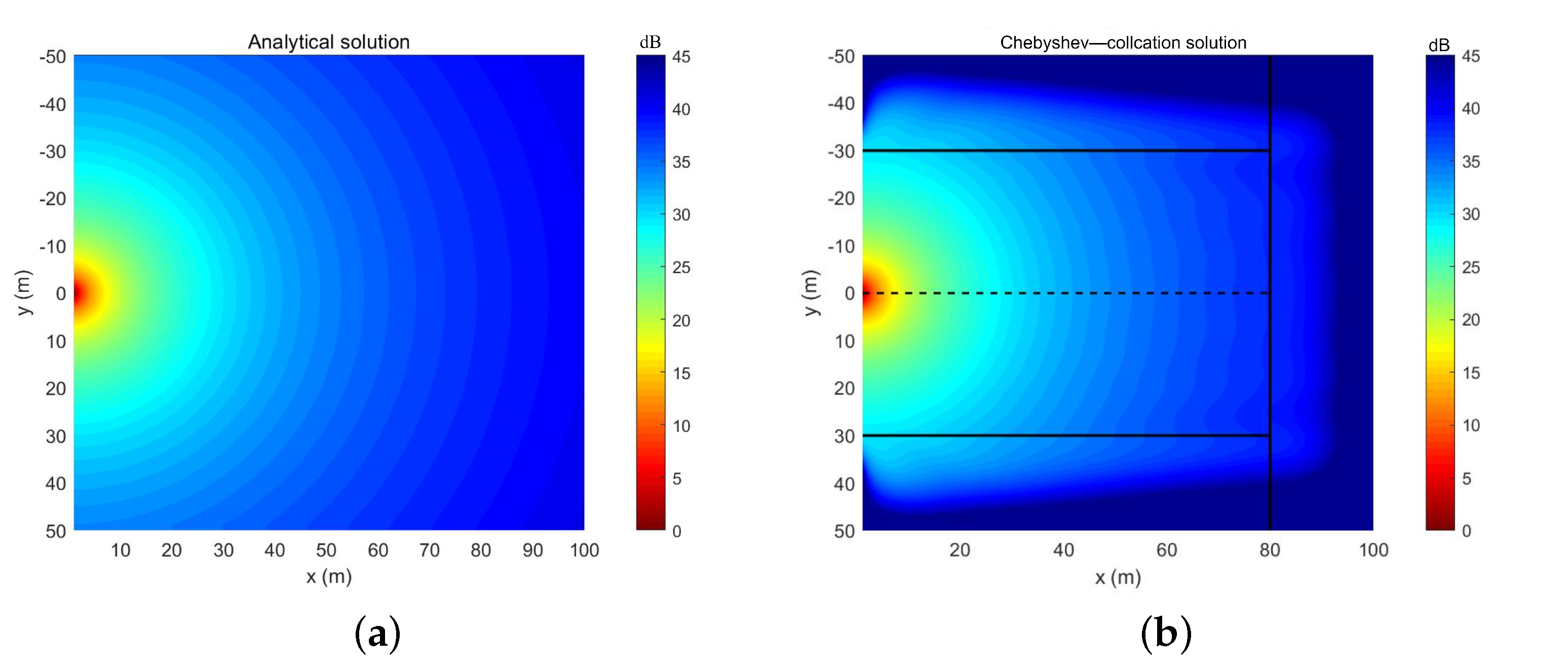
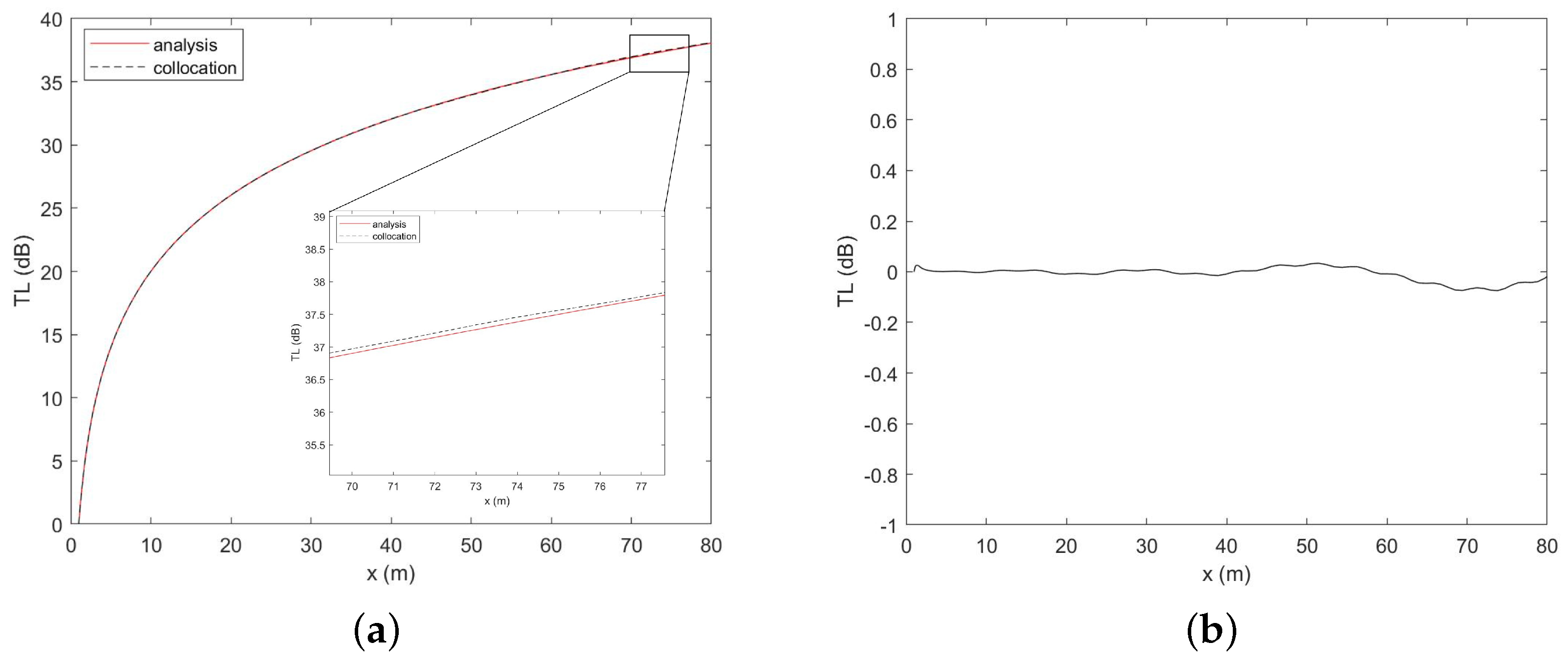
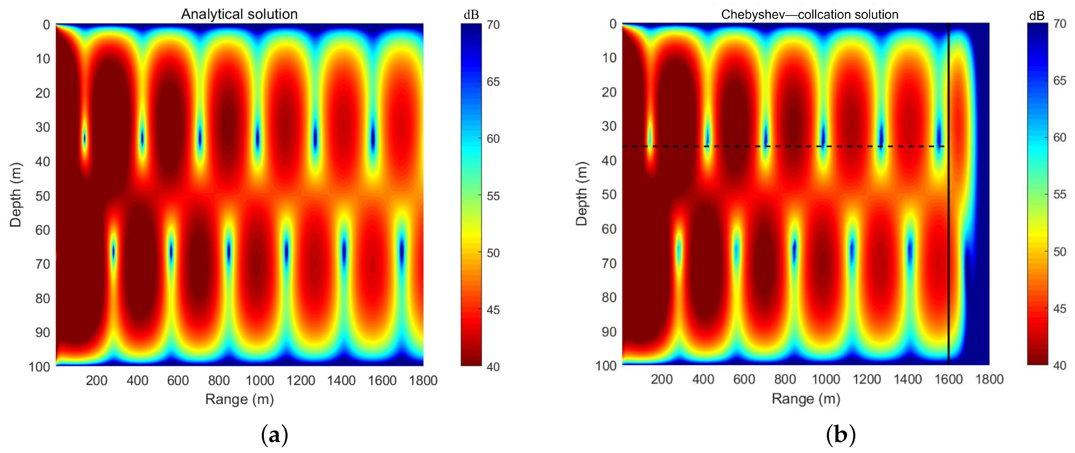
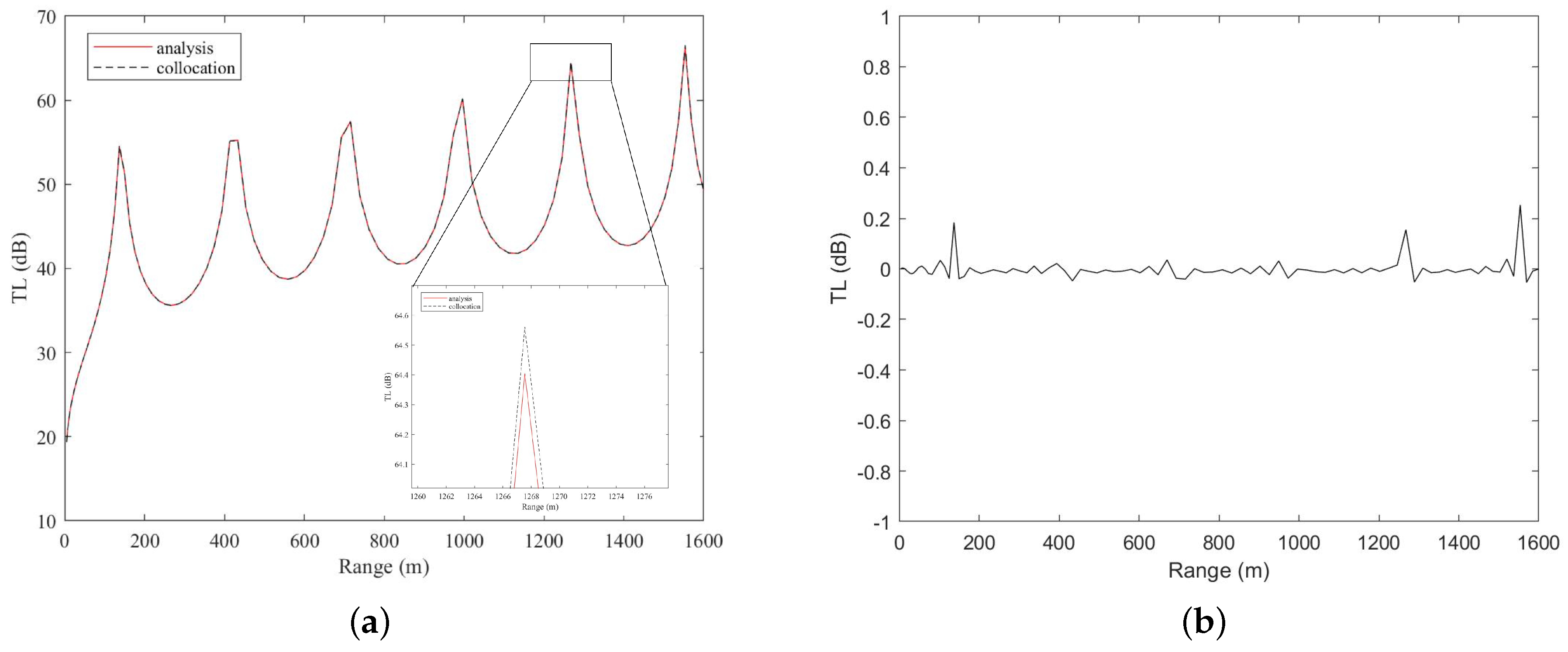
In this paper, the Chebyshev–Galerkin and Chebyshev–collocation spectral methods are used to directly solve the two-dimensional Helmholtz equation with Robin boundary conditions, and the results are compared with those of the corresponding analytical solutions. Because the Chebyshev–Galerkin spectral method requires trial functions to meet the boundary conditions, its boundary condition requirements are more stringent. In consideration of the complicated boundary conditions of the actual marine environment, the Chebyshev–collocation spectral method is used to solve the Helmholtz equation of two-dimensional ocean acoustic propagation. Similarly, the correctness of the method is verified by analytical solutions for an example of ocean acoustic propagation. Upon comparing the numerical calculation results of the collocation method with those of Kraken, the results show that the calculation accuracy of the collocation method is higher than that of Kraken. Therefore, it is feasible to use the spectral method to directly solve two-dimensional ocean acoustic propagation problems. The spectral method does not utilize simplified models, so there are no restrictions on the application conditions; thus, no approximation errors are introduced by the model. This method has a wide range of applications, high calculation accuracy, and high practical application value.

This paper is composed as follows. In Section 1, we introduce the current situation and main problems of ocean acoustic field solutions. Then, the Chebyshev–Galerkin and Chebyshev–collocation spectral methods are explained in Section 2 by applying them to solve the Helmholtz equation. In Section 3, we apply our method to the Helmholtz model equation and ocean acoustic program examples and analyze the results of the numerical calculations. Our conclusions are described in Section 4.

2. Solutions of the Two-Dimensional Helmholtz Equation

The basic idea of the spectral method is to approximately expand the solution of the problem on a cluster of smooth basis functions and convert the problem solved in the physical space into the problem of solving the expansion coefficient in the spectral space. The spectral method discretizes the differential equations in the entire solution domain into linear equations, and the core numerical algorithm is to solve the linear equations. In this section, we mainly study how to use the Chebyshev–Galerkin and Chebyshev–collocation spectral methods to directly solve the two-dimensional Helmholtz equation with Robin boundary conditions. Consider the two-dimensional boundary value problem:

$$\begin{array}{cc}\hfill & \frac{{\partial }^{2}u}{\partial x^2}+\frac{{\partial }^{2}u}{\partial y^2}+\alpha \frac{\partial u}{\partial x}+\beta \frac{\partial u}{\partial y}+\gamma u=f,-1\le x,y\le 1\hfill \\ \hfill & {\left.\left(u+k_1\frac{\partial u}{\partial x}\right)\right|}_{\left|x\right|=1}={\left.\left(u+k_2\frac{\partial u}{\partial y}\right)\right|}_{\left|y\right|=1}=0\hfill \end{array}$$

(1)

where $u(x,y)$ is the quantity to be solved and the other variables are known. When solving the above partial differential equations, first, it is necessary to discretize the equations to form an algebraic equation group that can be solved by mature numerical calculation methods. Here, we use the global approximation method, that is, the spectral method, to discretize the original equations. The continuous and smooth functions $u(x,y)$ and $f(x,y)$ in Equation (1) can be approximated by the linear combination of the complete and linearly independent function cluster ${\varphi }_{k,l}(x,y)$:

$$u\left(x,y\right)\approx \sum _{k=0}^N\sum _{l=0}^N{{\widehat{u}}_{k,l}\varphi }_{k,l}\left(x,y\right)$$

(2)

$$f\left(x,y\right)\approx \sum _{k=0}^N\sum _{l=0}^N{{\widehat{f}}_{k,l}\varphi }_{k,l}\left(x,y\right),$$

(3)

where ${\widehat{u}}_{k,l}$ and ${\widehat{f}}_{k,l}$ are coefficients of $u\left(x,y\right)$ and $f\left(x,y\right)$, respectively, and the function cluster ${\varphi }_{k,l}\left(x,y\right)$ is a two-dimensional trial function. ${\varphi }_{k,l}\left(x,y\right)$ can be expressed as the product of two one-dimensional trial functions:

$${\varphi }_{k,l}\left(x,y\right)={\varphi }_k\left(x\right){\varphi }_l\left(y\right).$$

(4)

In the Chebyshev–Galerkin and Chebyshev–collocation spectral methods, the two one-dimensional trial functions are both Chebyshev polynomials or their linear combinations.

2.1. The Definition and Properties of a One-Dimensional Chebyshev Polynomial

The Chebyshev polynomials $T_k\left(x\right)$ defined in the interval $[-1,+1]$ are:

$$T_k\left(x\right)=cos\left(k{cos}^{-1}(x\right))k=0,1,2\dots$$

(5)

Definition 1

(inner product and orthogonality). The Chebyshev polynomial cluster $\left\{T_k\left(x\right)\right\}$ satisfies the following (weighted) orthogonal relationship after introducing the following weighted inner product definition:

$${〈T_m,T_n〉}_{\omega }:={\int }_{-1}^{+1}{T}_m\left(x\right)T_n\left(x\right)w\left(x\right)dx=\left\{\begin{array}{c}0,m\ne n\\ \pi ,m=n=0\\ \frac{\pi }{2},m=n\ne 0\end{array}\right.$$

(6)

where the weight function $w\left(x\right)$ is:

$$w\left(x\right)=\frac{1}{\sqrt{1-x^2}}.$$

(7)

Define the coefficient $c_k$:

$$c_k=\left\{\begin{array}{c}2,k=0\\ 1,k>0\end{array}\right..$$

(8)

Considering the convenience of writing, if the polynomials are, at most, of the N-th power, Equation (6) can be rewritten in matrix form as:

$$\mathbf{K}=\mathit{diag}\left\{k_{ii}\right\},k_{ii}:=\frac{\pi }{2}{c}_k$$

(9)

where the matrix $\mathbf{K}$ is a diagonal matrix with dimensions of $\left(N+1\right)\times \left(N+1\right)$ and the diagonal element value is determined by $c_k$ in Equation (8).

Definition 2

(Chebyshev transform). The continuous smooth function $v\left(x\right)$ defined in the interval [−1,+1] can be approximately expanded with $T_k\left(x\right)$ as follows:

$$v\left(x\right)\approx \sum _{k=0}^N{{\widehat{v}}_{k}T}_k\left(x\right)$$

(10)

where N is the truncation order of the spectral method and ${\widehat{v}}_k$ is the Chebyshev expansion coefficient of function v. The expansion coefficient is:

$$\begin{array}{cc}\hfill & {\widehat{v}}_k=\frac{1}{d_k}{\int }_{-1}^{+1}v\left(x\right)T_k\left(x\right)w\left(x\right)dx,\hfill \\ \hfill & d_k={\int }_{-1}^{+1}\frac{T_k^2\left(x\right)}{\sqrt{1-x^2}}dx=\left\{\begin{array}{c}\pi ,k=0\\ \frac{\pi }{2},k>0\end{array}\right.\hfill \end{array}$$

(11)

Equations (10) and (11) are called the inverse and forward Chebyshev transforms [41]. If the effect of the truncation order is not taken into account, a one-to-one correspondence can be established between the original function $v\left(x\right)$ and its Chebyshev expansion coefficient $v_k$ using this pair of transformations, and they are located in the original physical space and spectral space.

Definition 3

(numerical integration method to calculate spectral expansion coefficient). In the forward Chebyshev transform Equation (11), the Gauss–Lobatto integral is usually used to calculate the weighted integral formula:

$${\widehat{v}}_k\approx \frac{1}{d_k}\sum _{i=0}^{N}v\left(x_i\right)T_k\left(x_i\right)w_i$$

(12)

where N is the number of integration nodes, which is taken as the truncation order of the spectral method. The integration nodes and weights are defined as:

$$x_0=1,x_N=-1,x_i=cos\left(\frac{\pi i}{N}\right),w_0=w_N=\frac{\pi }{2N},w_i=\frac{\pi }{N}$$

(13)

Definition 4

(the spectral coefficient of the derivative function). For any continuous smooth function $v\left(x\right)$ whose domain is [−1,+1], if the first derivative $v^{\prime }\left(x\right)$ of $v\left(x\right)$ is still a smooth function, $v^{\prime }\left(x\right)$ can also be expanded with $T_k\left(x\right)$ as:

$$v^{\prime }\left(x\right)\approx \sum _{k=0}^N{{\widehat{v}}_k^{\prime }T}_k\left(x\right)$$

(14)

It can be proven that the expansion coefficient ${\widehat{v}}_k^{\prime }$ of the first derivative of $v\left(x\right)$ and the expansion coefficient ${\widehat{v}}_k$ of the original function satisfy the following relationship [29]:

$${\widehat{v}}_k^{\prime }\approx \frac{2}{c_k}\sum _{\begin{array}{c}p=k+1\\ p+k=odd\end{array}}^{N}p{\widehat{v}}_p,k\ge 0$$

(15)

where $c_k$ is defined in Equation (8). Equation (15) can then be rewritten in matrix form:

$${\widehat{\mathbf{v}}}^{\prime }=\mathbf{D}\widehat{\mathbf{v}}$$

(16)

where ${\widehat{\mathbf{v}}}^{\prime }$ and $\widehat{\mathbf{v}}$ are $1\ast \left(N+1\right)$ arrays defined as: ${\widehat{\mathbf{v}}}^{\prime }=[{\widehat{v}}_0^{\prime },{\widehat{v}}_1^{\prime }\dots {\widehat{v}}_N^{\prime }]$ and $\widehat{\mathbf{v}}=\left[{\widehat{v}}_0,{\widehat{v}}_1\dots {\widehat{v}}_N\right]$. The matrix D is an upper triangular square matrix with dimensions of $\left(N+1\right)\times \left(N+1\right)$. Similarly, the expansion coefficient ${\widehat{\mathbf{v}}}^{″}$ of the second derivative $v^{″}\left(x\right)$ can be written as:

$${\widehat{\mathbf{v}}}^{″}={\mathbf{D}}^2\widehat{\mathbf{v}}$$

(17)

2.2. The Construction and Properties of One-Dimensional Chebyshev–Galerkin Trial Functions

In the one-dimensional Chebyshev–Galerkin spectral method, the construction of the trial function needs to satisfy not only the orthogonality described in Section 2.1 but also the boundary conditions of the equation to be solved. Therefore, in practice, the trial function ${\varphi }_k\left(x\right)$ is usually taken as the linear combination of the Chebyshev polynomial $T_k\left(x\right)$ and is called the Chebyshev–Galerkin trial function. Its general structure can be expressed as:

$${\varphi }_k\left(x\right)=T_k\left(x\right)+a_k{T}_{k+1}\left(x\right)+b_k{T}_{k+2}\left(x\right),k=0,1,2,\dots ,N-2$$

(18)

where the undetermined combination coefficients $a_k$ and $b_k$ can be determined by specific boundary conditions. In matrix form, Equation (18) can be rewritten as:

$$\left[\begin{array}{c}{\varphi }_0\left(x\right)\\ {\varphi }_1\left(x\right)\\ ⋮\\ {\varphi }_{N-2}\left(x\right)\end{array}\right]={\mathbf{S}}_x^T\left[\begin{array}{c}{T}_0\left(x\right)\\ T_1\left(x\right)\\ ⋮\\ T_N\left(x\right)\end{array}\right]$$

(19)

$${\mathbf{S}}_x^T=\left[\begin{array}{cccccc}1& a_k& b_k& & & \\ & 1& a_k& b_k& & \\ & & \ddots & \ddots & \ddots & \\ & & & 1& a_k& b_k\end{array}\right]$$

(20)

where the constant matrix ${\mathbf{S}}_x^T$ is a rectangular matrix with dimensions of $\left(N-1\right)\times \left(N+1\right)$.

Similar to the previous section, a series of properties of the Chebyshev–Galerkin trial functions can also be obtained. According to the orthogonality satisfied by the Chebyshev polynomials in Equations (6)–(9), the inner product of the Chebyshev–Galerkin trial functions can also be written in matrix form:

$$b_{k,j}={〈{\varphi }_j,{\varphi }_k〉}_{\omega },{\mathbf{B}}_x={\mathbf{S}}_x^T\mathbf{K}{\mathbf{S}}_x$$

(21)

where ${\mathbf{S}}_x$ is the transpose of matrix ${\mathbf{S}}_x^T$. The inner product of the Chebyshev trial function and Galerkin trial function can be written as:

$$h_{k,j}={〈T_j,{\varphi }_k〉}_{\omega },{\mathbf{H}}_x=\mathbf{K}{\mathbf{S}}_x$$

(22)

Similarly, the inner product of the Galerkin trial function and its derivative function can be written as:

$$c_{k,j}={〈{\varphi }_j^{\prime },{\varphi }_k〉}_{\omega },{\mathbf{C}}_x={\mathbf{S}}_x^T\mathbf{K}\mathbf{D}{\mathbf{S}}_x$$

(23)

$$a_{k,j}={〈{\varphi }_j^{″},{\varphi }_k〉}_{\omega },{\mathbf{A}}_x={\mathbf{S}}_x^T\mathbf{K}{\mathbf{D}}^2{\mathbf{S}}_x$$

(24)

2.3. Chebyshev–Galerkin Spectral Method for Solving the Two-Dimensional Helmholtz Equation

We first determine the two-dimensional Chebyshev–Galerkin trial function using Equations (4) and (18) and then discuss how to discretize Equation (1). According to the principle of the MWR, it is necessary to approximate the value of the function u to be solved using the Chebyshev–Galerkin trial function for a finite N-term expansion and then make the residual of the equation orthogonal to the space of the test function; that is, the weighted inner products of the residual and each test function are zero. According to Equation (1), we can obtain:

$$\begin{array}{cc}\hfill & {〈\frac{{\partial }^{2}u}{\partial x^2},{\phi }_{k,l}〉}_{\omega }+{〈\frac{{\partial }^{2}u}{\partial y^2},{\phi }_{k,l}〉}_{\omega }+\alpha {〈\frac{\partial u}{\partial x},{\phi }_{k,l}〉}_{\omega }+\hfill \\ \hfill & \beta {〈\frac{\partial u}{\partial y},{\phi }_{k,l}〉}_{\omega }+\gamma {〈u,{\phi }_{k,l}〉}_{\omega }={〈f,{\phi }_{k,l}〉}_{\omega }\hfill \end{array}$$

(25)

where ${\phi }_{k,l}$ represents the two-dimensional test function. According to the different methods used in the test function, the spectral method discussed in this paper can be further divided into the Chebyshev–Galerkin spectral method and the Chebyshev–collocation spectral method.

In the Chebyshev–Galerkin spectral method, the test function is taken as the Chebyshev–Galerkin trial function itself. Therefore, each item in Equation (25) can be expressed in a concise matrix form. For instance, the inner product of the second-derivative term is:

$$\begin{array}{cc}\hfill & {〈\frac{{\partial }^{2}u}{\partial x^2},{\phi }_{k,l}〉}_{\omega }={〈\sum _{m=0}^N\sum _{n=0}^N{\widehat{u}}_{m,n}{\varphi }_m^{{}^{″}}\left(x\right){\varphi }_n\left(y\right),{\varphi }_k\left(x\right){\varphi }_l\left(y\right)〉}_{\omega }\hfill \\ \hfill & =\sum _{m=0}^N\sum _{n=0}^N{\widehat{u}}_{m,n}{\int \int }_{-1}^{+1}{\varphi }_m^{{}^{″}}\left(x\right){{\varphi }_k\left(x\right){w\left(x\right)\varphi }_n\left(y\right)\varphi }_l\left(y\right)w\left(y\right)dxdy\hfill \\ \hfill & =\sum _{m=0}^N\sum _{n=0}^N{\widehat{u}}_{m,n}{〈{\varphi }_m^{{}^{″}}\left(x\right),{\varphi }_k\left(x\right)〉}_{\omega }{〈{{\varphi }_n\left(y\right),\varphi }_l\left(y\right)〉}_{\omega }={\mathbf{A}}_x\mathbf{U}{\mathbf{B}}_y^T.\hfill \end{array}$$

(26)

Similarly:

$${〈\frac{{\partial }^{2}u}{\partial y^2},{\phi }_{k,l}〉}_{\omega }={\mathbf{B}}_x\mathbf{U}{\mathbf{A}}_y^T$$

(27)

The inner product of the first-derivative term can be rewritten as:

$$\begin{array}{cc}\hfill & {〈\frac{\partial u}{\partial x},{\phi }_{k,l}〉}_{\omega }={〈\sum _{m=0}^N\sum _{n=0}^N{\widehat{u}}_{m,n}{\varphi }_m^{{}^{\prime }}\left(x\right){\varphi }_n\left(y\right),{\varphi }_k\left(x\right){\varphi }_l\left(y\right)〉}_{\omega }\hfill \\ \hfill & =\sum _{m=0}^N\sum _{n=0}^N{\widehat{u}}_{m,n}{\int \int }_{-1}^{+1}{\varphi }_m^{{}^{\prime }}\left(x\right){{\varphi }_k\left(x\right){w\left(x\right)\varphi }_n\left(y\right)\varphi }_l\left(y\right)w\left(y\right)dxdy\hfill \\ \hfill & =\sum _{m=0}^N\sum _{n=0}^N{\widehat{u}}_{m,n}{〈{\varphi }_m^{{}^{\prime }}\left(x\right),{\varphi }_k\left(x\right)〉}_{\omega }{〈{{\varphi }_n\left(y\right),\varphi }_l\left(y\right)〉}_{\omega }={\mathbf{A}}_x\mathbf{U}{\mathbf{B}}_y^T.\hfill \end{array}$$

(28)

Similarly:

$${〈\frac{\partial u}{\partial y},{\phi }_{k,l}〉}_{\omega }={\mathbf{B}}_x\mathbf{U}{\mathbf{C}}_y^T$$

(29)

The inner product of the original-function term can be rewritten as:

$$\begin{array}{cc}\hfill & {〈u,{\phi }_{k,l}〉}_{\omega }={〈\sum _{m=0}^N\sum _{n=0}^N{\widehat{u}}_{m,n}{\varphi }_m\left(x\right){\varphi }_n\left(y\right),{\varphi }_k\left(x\right){\varphi }_l\left(y\right)〉}_{\omega }\hfill \\ \hfill & =\sum _{m=0}^N\sum _{n=0}^N{\widehat{u}}_{m,n}{\int \int }_{-1}^{+1}{\varphi }_m\left(x\right){{\varphi }_k\left(x\right){w\left(x\right)\varphi }_n\left(y\right)\varphi }_l\left(y\right)w\left(y\right)dxdy\hfill \\ \hfill & =\sum _{m=0}^N\sum _{n=0}^N{\widehat{u}}_{m,n}{〈{\varphi }_m\left(x\right),{\varphi }_k\left(x\right)〉}_{\omega }{〈{{\varphi }_n\left(y\right),\varphi }_l\left(y\right)〉}_{\omega }={\mathbf{B}}_x\mathbf{U}{\mathbf{B}}_y^T.\hfill \end{array}$$

(30)

The inner product of the right-hand-side known-function term is:

$$\begin{array}{cc}\hfill & {〈f,{\phi }_{k,l}〉}_{\omega }=\sum _{m=0}^{N+2}\sum _{n=0}^{N+2}{\widehat{f}}_{m,n}{〈T_m\left(x\right)T_n\left(x\right),{{\varphi }_k\left(x\right)\varphi }_l\left(y\right)〉}_{\omega }\hfill \\ \hfill & =\sum _{m=0}^{N+2}\sum _{n=0}^{N+2}{\widehat{f}}_{m,n}{〈T_m\left(x\right),{\varphi }_k\left(x\right)〉}_{\omega }{〈{T_n\left(y\right),\varphi }_l\left(y\right)〉}_{\omega }={\mathbf{H}}_x^T\widehat{\mathbf{f}}{\mathbf{H}}_y.\hfill \end{array}$$

(31)

where $\widehat{\mathbf{f}}$ is the spectral expansion coefficient of the known function f under the Chebyshev trial function in Equation (1) and $\mathbf{U}$ is the spectral expansion coefficient of the unsolved quantity $u\left(x,y\right)$ under the Galerkin trial function. Substituting Equations (26)–(31) into Equation (25) gives:

$${\mathbf{A}}_x\mathbf{U}{\mathbf{B}}_y^T+{\mathbf{B}}_x\mathbf{U}{\mathbf{A}}_y^T+\alpha {\mathbf{C}}_x\mathbf{U}{\mathbf{B}}_y^T+\beta {\mathbf{B}}_x\mathbf{U}{\mathbf{C}}_y^T+\gamma {\mathbf{B}}_x\mathbf{U}{\mathbf{B}}_y^T={\mathbf{H}}_x^T\widehat{\mathbf{f}}{\mathbf{H}}_y$$

(32)

To solve $\mathbf{U}$ conveniently, the two-dimensional matrices $\mathbf{U}$ and $\widehat{\mathbf{f}}$ are compressed into one-dimensional vectors by columns, which are denoted as $\overline{\mathbf{u}}$ and $\overline{\mathbf{f}}$, respectively. Equation (32) can be rewritten as:

$$\left({\mathbf{B}}_y\otimes {\mathbf{A}}_x+{\mathbf{A}}_y\otimes {\mathbf{B}}_x+\alpha {\mathbf{B}}_y\otimes {\mathbf{C}}_x+\beta {\mathbf{C}}_y{\otimes \mathbf{B}}_x+\gamma {\mathbf{B}}_y\otimes {\mathbf{B}}_x\right)\overline{\mathbf{u}}={\mathbf{H}}_y^T\otimes {\mathbf{H}}_x^T\overline{\mathbf{f}}$$

(33)

where ⊗ is the Kronecker product. This is a linear equation system for the unknown vector $\overline{\mathbf{u}}$, which can be solved by using standard numerical methods to obtain the expansion coefficient $\overline{\mathbf{u}}$ of the function $u\left(x,y\right)$. Then, we can obtain the value of the function $u\left(x,y\right)$ according to Equation (2).

2.4. Chebyshev–Collocation Spectral Method for Solving the Two-Dimensional Helmholtz Equation

In Equation (25), if the test function cluster is selected as the following special function, it is called the Chebyshev–collocation spectral method. Taking the x direction as an example, specific $(N+1)$ points ${\left\{x_j\right\}}_{j=0}^N$ in the solution domain are selected as collocation points, and the $\delta$ function ($\delta \left(x\right)=0,(x\ne 0)$) is used as the weight function:

$$w_j\left(x\right)=\delta \left(x-x_j\right)$$

(34)

According to the principle of the MWR, the residual is required to be zero at the $\left(N+1\right)$ collocation points, which means that the differential equation is strictly established at the $\left(N+1\right)$ collocation points.

It is still possible to discretize a system of equations in spectral space, as discussed in Section 2.2, and then transform them back to physical space to obtain approximate solutions of the original equations. However, due to the feature of the test function, the Chebyshev–collocation spectral method can directly form a system of equations in the original physical space without having to resort to spectral space. Because of this feature, the collocation-type spectral method can easily address variable coefficients and nonlinear problems. We discuss this method and solution in detail as follows.

The calculation of the collocation-type spectral method is mainly carried out in grid-point space, and the calculation accuracy is related to the selection of the collocation point. For convenience, the Gauss–Lobatto node is selected as the grid collocation point, and the detailed definition is shown in Equation (13). First, we construct the Chebyshev derivative matrix. On the discrete point, x is used to represent the $\left(N+1\right)$ dimensional vector composed of discrete point coordinates, and $\mathbf{u}$ is used to represent the $\left(N+1\right)$ dimensional vector composed of the function values at these points. Then the $\left(N+1\right)\times \left(N+1\right)$ Chebyshev derivative matrix $\tilde{\mathbf{D}}$ satisfies:

$${\mathbf{u}}^{\prime }\left(x\right)=\tilde{\mathbf{D}}\mathbf{u}$$

(35)

Similarly, the second-order derivative matrix is ${\tilde{\mathbf{D}}}^2$.

The function u in Equation (1) is discretized at the collocation points. Similar to the solution process of the Galerkin method, if the function u is compressed into a one-dimensional vector in columns, then Equation (1) on the left-hand side can be rewritten as:

$$\frac{{\partial }^2}{\partial x^2}\to {\tilde{\mathbf{D}}}_N^2\otimes {\mathbf{I}}_{M+1}$$

(36)

$$\frac{{\partial }^2}{\partial y^2}\to {\mathbf{I}}_{N+1}\otimes {\tilde{\mathbf{D}}}_M^2$$

(37)

$$\alpha \frac{\partial }{\partial x}\to \alpha {\tilde{\mathbf{D}}}_N\otimes {\mathbf{I}}_{M+1}$$

(38)

$$\beta \frac{\partial }{\partial y}\to \beta {\mathbf{I}}_{N+1}\otimes {\tilde{\mathbf{D}}}_M$$

(39)

$$\gamma \to \gamma {\mathbf{I}}_{\left(N+1\right)(M+1)}$$

(40)

where the number of discrete points in the x direction is $\left(N+1\right)$, that in the y direction is $\left(M+1\right)$, and ${\mathbf{I}}_M$ is an M-order identity matrix. The matrix forms of the boundary conditions ${\mathbf{R}}_x$ and ${\mathbf{R}}_y$ are as follows:

$$u+k_1\frac{\partial u}{\partial x}\to {\mathbf{R}}_x{\mathbf{u}}_{\left(N+1\right)\left(M+1\right)}={\mathbf{I}}_{\left(N+1\right)\left(M+1\right)}+k_1\left({\tilde{\mathbf{D}}}_N\otimes {\mathbf{I}}_{M+1}\right)$$

(41)

$$u+k_2\frac{\partial u}{\partial y}\to {\mathbf{R}}_y{\mathbf{u}}_{\left(N+1\right)\left(M+1\right)}={\mathbf{I}}_{\left(N+1\right)\left(M+1\right)}+k_2\left({\mathbf{I}}_{N+1}\otimes {\tilde{\mathbf{D}}}_M\right)$$

(42)

The rows of the matrices ${\mathbf{R}}_x$ and ${\mathbf{R}}_y$ corresponding to the boundaries $\left|x\right|=1$ and $\left|y\right|=1$ are placed into the corresponding positions in matrix $\mathbf{L}$ (Equation (43)).

$$\begin{array}{cc}\hfill & \frac{{\partial }^2}{\partial x^2}+\frac{{\partial }^2}{\partial y^2}+\alpha \frac{\partial }{\partial x}+\beta \frac{\partial }{\partial y}+\gamma \to \mathbf{L}\hfill \\ \hfill & \mathbf{L}={\tilde{\mathbf{D}}}_N^2\otimes {\mathbf{I}}_{M+1}+{\mathbf{I}}_{N+1}\otimes {\tilde{\mathbf{D}}}_M^2+\alpha {\tilde{\mathbf{D}}}_N\otimes {\mathbf{I}}_{M+1}+\beta {\mathbf{I}}_{N+1}\otimes {\tilde{\mathbf{D}}}_M+\gamma {\mathbf{I}}_{\left(N+1\right)\left(M+1\right)}\hfill \end{array}$$

(43)

The symbol “-” above $\mathbf{L}$ indicates the modified matrix operator. Then, Equation (44) is solved to obtain $\mathbf{u}$.

$${\mathbf{u}}_{\left(N+1\right)\left(M+1\right)\times 1}={\overline{\mathbf{L}}}^{-1}\overline{\mathbf{f}}$$

(44)

where the vector $\mathbf{f}$ is a discretized description of $f(x,y)$. $\overline{\mathbf{f}}$ is modified as follows: the elements at the boundary $\left|x\right|=1$ and $\left|y\right|=1$ are taken as zero (according to the boundary conditions of Equation (1)).

3. Numerical Test and Results Analysis

In this section, we first apply the Chebyshev–Galerkin and Chebyshev–collocation spectral methods to solve the two-dimensional model Helmholtz equation and then compare the results and calculation times of the two numerical calculations. Since the Chebyshev–collocation spectral method has a wide range of applications and does not require strict boundary conditions as Galerkin method, it is applied to solve actual ocean acoustic calculation examples, and analytical solutions are used to verify the correctness of the numerical results. Then, we compare the numerical calculation results of the collocation method with those of Kraken to improve the calculation accuracy. The truncation order N in the two directions is not required to be the same; however, to facilitate this test, the N values in the two directions are assumed to be the same in the numerical experiments. In the following, N refers to the truncation order in one direction unless otherwise specified. The numerical calculation program is written in GNU Octave code, and the test platform is a Dell XPS8930 desktop computer equipped with an Intel i7-8700K CPU and 32 GB of memory.

3.1. Two-Dimensional Model Helmholtz Equation

In this section, we take the solution of the following model equation as an example for numerical testing and analysis.

$$\begin{array}{cc}\hfill & \frac{{\partial }^{2}u}{\partial x^2}+\frac{{\partial }^{2}u}{\partial y^2}+\frac{\partial u}{\partial x}+\frac{\partial u}{\partial y}+u=f,(x,y)\in (-1,1)\times (-1,1)\hfill \\ \hfill & {\left.u-\frac{1}{\pi }\frac{\partial u}{\partial x}\right|}_{\left|x\right|=1}={\left.u-\frac{1}{2\pi }\frac{\partial u}{\partial y}\right|}_{\left|y\right|=1}=0\hfill \\ \hfill & f\left(x,y\right)=\left(-5{\pi }^2+1\right)sin\left(\pi x+\frac{\pi }{4}\right)sin\left(2\pi y+\frac{\pi }{4}\right)+\pi cos\left(\pi x+\frac{\pi }{4}\right)sin\left(2\pi y+\frac{\pi }{4}\right)\hfill \\ \hfill & +2\pi sin\left(\pi x+\frac{\pi }{4}\right)cos\left(2\pi y+\frac{\pi }{4}\right)\hfill \end{array}$$

(45)

The exact solution of Equation (45) is $u=sin(\pi x+\frac{\pi }{4})sin\left(2\pi y+\frac{\pi }{4}\right)$.

Equation (45) is solved by the Chebyshev–Galerkin and Chebyshev–collocation spectral methods, and the approximate solution images obtained are shown in Figure 1. The accuracy is determined by the relative L${}_2$-norm of the error between the numerical solution and the exact solution and the definition of L${}_2$-norm of vector $\mathbf{x}$ are:

$$\begin{array}{cc}\hfill & \mathrm{error}=\frac{{∥u-u_{\mathrm{ana}}∥}_2}{{∥u_{\mathrm{ana}}∥}_2}\hfill \\ \hfill & {∥\mathbf{x}∥}_2=\sqrt{{\left|x_1\right|}^2+{\left|x_2\right|}^2+{\left|x_3\right|}^2+\dots +{\left|x_n\right|}^2}\hfill \end{array}$$

(46)

where ${∥·∥}_2$ represents the L${}_2$-norm of the error, u represents numerical results, and $u_{\mathrm{ana}}$ represents the exact solution.

Figure 1 shows the images of the exact solution and the numerical solutions of the two methods. This function has good smoothness and symmetry, but the image is more complex, and the gradient changes greatly.

Table 1. The error of the results calculated by the Chebyshev–Galerkin and Chebyshev–collocation spectral methods varies with the truncation order N.

N	Galerkin Error	Collocation Error
8	$1.19\times {10}^{-5}$	$5.60\times {10}^{-2}$
16	$2.73\times {10}^{-6}$	$2.68\times {10}^{-6}$
22	$5.62\times {10}^{-11}$	$6.24\times {10}^{-11}$
24	$1.04\times {10}^{-12}$	$2.84\times {10}^{-12}$
30	$2.51\times {10}^{-14}$	$8.15\times {10}^{-12}$
32	$2.57\times {10}^{-14}$	$5.51\times {10}^{-12}$

shows that the two spectral methods show a similar order of accuracy until $N=24$. At $N=30$, all the numerical solutions nearly reach the machine accuracy (∼10${}^{-16}$) under double precision. This shows that these two methods can obtain high-precision approximate solutions when the truncation order N is small, which verifies the high-precision approximation of the spectral method. The approximation accuracy of the two numerical methods increases rapidly with increasing truncation order. For almost every increase in order, the accuracy of the numerical solution increases by an order of magnitude, which verifies the rapid convergence of the spectral method. The Chebyshev–Galerkin method achieves the highest accuracy at $N=30$, when the error magnitude is ${10}^{-14}$, and the Chebyshev–collocation method achieves the highest accuracy at $N=24$, when the error magnitude is ${10}^{-12}$. By comparison, the two spectral methods are both high-precision calculation methods. However, the Chebyshev–collocation spectral method uses fewer orders to achieve the highest accuracy and can effectively reduce the amount of calculation required to solve complex and large-scale problems.

The calculation times of the Chebyshev–Galerkin and Chebyshev–collocation methods vary with N, as shown in

Table 2. The calculation times of the Chebyshev–Galerkin and Chebyshev–collocation methods vary with N.

N	Galerkin Time (s)	Collocation Time (s)
8	0.007	0.003
16	0.014	0.005
22	0.020	0.008
24	0.023	0.010
30	0.032	0.022
32	0.042	0.025

. The results listed in the table are the average results of ten runs. The running time results of the two spectral methods show that the Chebyshev–collocation method runs faster than the Chebyshev–Galerkin spectral method. Comparing the calculation errors of these two methods, the Chebyshev–collocation method can achieve a higher calculation accuracy in a shorter time and with less truncation order. Therefore, compared to the Chebyshev–Galerkin method, the Chebyshev–collocation method can calculate more quickly and efficiently while ensuring accuracy when solving realistic problems of ocean acoustic propagation. In addition, the Galerkin-type spectral method requires trial functions to meet the boundary conditions, and the corresponding trial functions need to be designed for specific boundary conditions. However, when solving realistic ocean acoustic field problems, the construction of the Galerkin trial function is very difficult if the boundary conditions change with distance. Therefore, the next section introduces the application of the Chebyshev–collocation spectral method in solving realistic ocean acoustic fields.

3.2. Ocean Acoustic Propagation Example Test

The test in Section 3.1 verified that the Chebyshev–collocation spectral method directly solves the two-dimensional Helmholtz model equation with a high accuracy and fast convergence. Therefore, we apply it to solve the two-dimensional ocean acoustic propagation equation. Two ocean acoustic propagation examples, spherical waves and ideal fluid waveguides, with analytical solutions are selected for analysis and comparison to verify the effectiveness of the Chebyshev–collocation method in solving the ocean acoustic field.

When the ocean topography and ocean environment parameters are axisymmetric, the circumferential guide number in the cylindrical coordinate system is zero, that is, $\partial /\partial \theta =0$. The Helmholtz equation in cylindrical coordinates can be simplified into a two-dimensional axisymmetric form [13]:

$$\frac{\partial }{\partial r}\left(\frac{1}{\rho }\frac{\partial P}{\partial r}\right)+\frac{1}{r\rho }\frac{\partial P}{\partial r}+\frac{\partial }{\partial z}\left(\frac{1}{\rho }\frac{\partial P}{\partial z}\right)+\frac{k^{2}P}{\rho }=0$$

(47)

where P is the sound pressure, $\rho$ is the density, k is the wavenumber, r is the horizontal axis, and z is the vertical axis. The boundary conditions are also required to obtain the specific sound pressure distribution. To simulate the sound field characteristics of a real large-scale sea area, it is often necessary to set the radiation boundary conditions, that is, the conditions that the solution of the wave equation needs to meet at infinity (the sound propagation direction at infinity can only be outward). The Sommerfeld radiation condition expression is:

$$\frac{\partial P}{\partial n}-ikP=0$$

(48)

This condition indicates that on the virtual boundary far from the sound source point, the normal derivative of sound pressure and the sound pressure itself satisfy Equation (48).

The premise of the radiation boundary conditions is that that they correspond to an infinite distance from the sound source point. However, due to the limitation of the calculation area, an “absorption layer” needs to be set at the boundary to avoid false reflections of the sound field by the radiation boundary conditions. The inner side of the absorption layer is connected to the sound field, and the radiation boundary condition is set on the outer side. The absorption coefficient in the absorption layer increases rapidly with increasing coordinate values, such that the sound pressure can be rapidly reduced within a short distance. The wavenumber expression in the absorption layer [13] is:

$$\begin{array}{cc}\hfill & K^2=k^2\left[1+i\left({\gamma }_r+{\gamma }_z+\frac{\beta }{27.287527}\right)\right]\hfill \\ \hfill & {\gamma }_r=\left\{\begin{array}{c}0,r\le L\\ \mu \left(\frac{r-L}{▵L}{)}^2,r>L\right.\end{array}\right.{\gamma }_z=\left\{\begin{array}{c}0,z\le H\\ \mu \left(\frac{z-H}{▵H}{)}^2,z>H\right.\end{array}\right.\hfill \end{array}$$

(49)

where the coefficient $\mu$ is usually zero, ${\gamma }_r$ represents the change coefficient of the absorption layer in the horizontal direction, ${\gamma }_z$ represents the change coefficient of the absorption layer in the vertical direction, L represents the horizontal coordinate of the inner side of the absorption layer in the horizontal direction, and H represents the vertical coordinate of the inner side of the absorption layer in the vertical direction. To simulate real ocean conditions, the absorption coefficient $\beta$ is zero.

To show the calculation results of the sound field, the transmission loss of the sound pressure is defined as:

$$\mathrm{TL}=-20{log}_{10}\left(\frac{\left|P\right|}{P_0}\right)$$

(50)

where $P_0$ refers to the sound pressure 1 m from the sound source. In displays of sound field results, TL is commonly used, and the unit of TL is decibels(dB).

3.2.1. Spherical Wave

The density of the ocean is uniform $\rho \left(z\right)=1$ g/cm${}^3$, the speed of underwater sound propagation is constant $c=1500$ m/s, the sound source is set at the coordinate origin (0,0), and the frequency is 150 Hz. To avoid singularities in the calculation area, the horizontal solution area is (1, 100), and the vertical solution area is (−50, 50). The analytical solution of the spherical wave is:

$$P=\frac{e^{ikR}}{R},R=\sqrt{x^2+y^2}$$

(51)

The upper boundary, lower boundary and right boundary of the solved rectangular area are all assigned radiation conditions, and the thicknesses of the three boundary absorption layers are all 20 m. The left boundary is described by the analytical solution formula.

The truncation order $N=160$ is taken as an example to focus on the nonabsorbent layer area, that is, (1, 80) in the horizontal direction and (−30, 30) in the vertical direction. The corresponding calculation results are shown in Figure 2.

Figure 2 shows that the sound field value calculated by the Chebyshev–collocation spectral method in the nonabsorbent layer area is very similar to the results calculated by the analytical solution. However, due to the influence of the radiation conditions, strong reflections are generated near the boundary, resulting in a certain jitter in the sound field value near the inner boundary. Upon comparing the TLs at the sound source depth computed by the analytical solution (red solid line) with the results by the collocation method (black dashed line), as shown in Figure 3a, the TLs are basically the same. Figure 3b shows the error between the numerical solution and the analytical solution. Figure 3 shows that there is a slight difference in the calculation results of the collocation method in the area beyond 60 m due to the reflection of the radiation boundary.

We use the analytical solution of spherical waves to analyze the accuracy of the numerical calculation results. The analysis is focused on the result in the nonabsorbent layer, so the absorption layer is ignored. The error between the numerically calculated sound field and the analytical solution is measured by the relative L${}_2$-norm defined by Equation (46).

Table 3. The numerical calculation error of the entire solution domain and the depth of the sound source vary with N.

N	Error in the Entire Domain	Error at the Depth of the Sound Source
60	$1.32700463\times {10}^{-1}$	$1.34443432\times {10}^{-1}$
80	$4.73780863\times {10}^{-3}$	$4.87139228\times {10}^{-3}$
100	$2.09898576\times {10}^{-3}$	$2.08030059\times {10}^{-3}$
120	$1.64301023\times {10}^{-3}$	$1.17537743\times {10}^{-3}$
140	$1.54173280\times {10}^{-3}$	$9.60149598\times {10}^{-4}$
160	$1.48522444\times {10}^{-3}$	$9.31331082\times {10}^{-4}$

shows the error in the entire solution domain (except the absorption layer), and the depth of the sound source varies with the number of discrete points N. Table 3 also shows that with the increase in N, the calculation error of the Chebyshev–collocation spectral method gradually decreases, and the numerical calculation accuracy gradually improves.

We analyze the execution time of the spectral method as the scales of problem change. We guarantee that the calculation error in the whole solution domain is on the order of ${10}^{-3}$. Then, the speed of sound and the size of the solution domain are fixed, the frequency of the sound source is changed, and the variation in the execution time with the wavenumber changing in the solution domain is analyzed. Under the premise of ensuring accuracy,

Table 4. The truncation order N and the execution time vary with the frequency of the sound source.

Frequency (Hz)	N	Execution Time (s)
150	100	14.1058
300	110	27.5516
400	130	77.5650
450	137	105.7993
500	145	145.8439

shows the change in the truncation order N and the execution time of the program with the frequency of the sound source. According to Table 4, as the frequency increases, the wavelength decreases, and the wavenumber contained in the solution domain increases. To ensure the calculation accuracy, the value of N must be increased, which also makes the scale of the discrete matrix $\mathbf{L}$ of Equation (43) further increase. Similarly, the scale of solving linear equations of Equation (44) increases, which leads to an increase in the execution time.

3.2.2. Ideal Fluid Waveguide

The density of the ocean is uniform at $\rho \left(z\right)=1$ g/cm${}^3$, the speed of underwater sound propagation is constant at $c=1500$ m/s, the sound source is at a depth of 36 m, and the frequency is 20 Hz. The upper and lower boundaries of the solved rectangular area are the pressure release boundary conditions, the left boundary is described by analytical solutions, and the right boundary is described by the radiation boundary condition. The thickness of the absorption layer is 200 m. Therefore, we mainly analyze the calculation area within 1600 m in the horizontal direction. The truncation order $N=120$ is considered, and the result is shown in Figure 4.

Figure 4 shows that the sound field solution of the nonabsorbent layer calculated by the collocation method is very similar to the analytical solution but that there is a small difference in the position of the sound shadow area. Figure 5 shows the TL curves of the two calculation methods at a sound source depth of 36 m. The calculation results of the collocation method and the analytical solution are very similar, but there is a certain error in the sound shadow area. The result in the sound shadow area is relatively complicated, and the calculation is difficult, which leads to errors in the calculation of the collocation method. The analytical solution of the ideal fluid wave is used to analyze the accuracy of the numerical calculation in the nonabsorbent layer region, and the results are shown in

Table 5. The numerical calculation error in the entire solution domain varies with N.

N	Chebyshev–Collocation	Kraken
70	$2.06853038\times {10}^{-1}$	$2.41551098\times {10}^{-1}$
80	$5.67631508\times {10}^{-4}$	$2.41551093\times {10}^{-1}$
100	$7.09835092\times {10}^{-4}$	$2.41551112\times {10}^{-1}$
120	$4.75639831\times {10}^{-4}$	$2.41551129\times {10}^{-1}$

. The results in Table 5 indicate that when the value of N increases to 80, the accuracy of the numerical calculation can reach ${10}^{-4}$. This example is also solved by the classic Kraken program based on the normal mode method. As shown in Table 5, even if the number of discrete points is increased, the magnitude of the error is still ${10}^{-1}$, a very important reason is that Kraken program uses the normal mode approximation does not accurately reproduce the field near the sound source.

Table 6. The numerical calculation error at the sound source depth varies with N.

N	Chebyshev–Collocation	Kraken
70	$3.32036066\times {10}^{-1}$	$2.06786673\times {10}^{-3}$
80	$1.52415237\times {10}^{-3}$	$2.06475574\times {10}^{-3}$
100	$1.73634299\times {10}^{-3}$	$2.06635146\times {10}^{-3}$
120	$9.33660302\times {10}^{-4}$	$2.06476704\times {10}^{-3}$

shows the errors of the two numerical calculation methods at the sound source depth of 36 m. The calculation accuracy of the collocation method is lower at $N=70$, and the results of Kraken reach a higher accuracy of approximately ${10}^{-3}$. The calculation accuracy of the collocation method is rapidly improved with increasing N. At $N=120$, the accuracy of the collocation method exceeds that of Kraken by approximately ${10}^{-4}$. Comparative analysis indicates that the accuracy of the Chebyshev–collocation method is higher than that of Kraken, which verifies the high-precision characteristics of the spectral method. For the above two calculation examples with complex boundary conditions, the Chebyshev–collocation spectral method can achieve a higher calculation accuracy when the truncation order is small. For ocean acoustic propagation examples with complex boundaries and propagation characteristics that are difficult to solve by other methods, the Chebyshev–collocation spectral method can be solved efficiently and accurately.

4. Conclusions and Outlook

This paper uses the Chebyshev–Galerkin and Chebyshev–collocation spectral methods to directly solve two-dimensional Helmholtz model equations and uses an analytical solution to verify the correctness of the two methods. The Chebyshev–Galerkin spectral method first constructs a trial function that satisfies the boundary conditions, then interpolates at the Gauss–Lobatto node, forms a system of linear equations in the spectral space, and finally obtains the original function. However, the two-dimensional ocean acoustic propagation Helmholtz equation is relatively complicated due to the variable boundary conditions, and the trial function is difficult to construct. Therefore, realistic ocean acoustic examples can be solved by the more widely applicable Chebyshev–collocation spectral method. The Chebyshev–collocation spectral method approximates the function value at the Gauss–Lobatto node, interpolates physical quantities such as the boundary conditions and sound velocity to the Gauss–Lobatto node, and then directly solves the system of linear equations in the physical space to obtain the original function. The analytical solution is used to verify the correctness of the Chebyshev–collocation method, and compared with the classic Kraken program, the Chebyshev–collocation method has a higher calculation accuracy. The Chebyshev–collocation method can be used to directly solve the two-dimensional underwater acoustic propagation Helmholtz equation without being restricted and constrained by other simplified model application conditions and will not introduce model errors. This spectral method can be used to solve the situation where the sound velocity in the domain changes with the horizontal and vertical directions, and it is applicable to Dirichlet Neumann and Robin boundary conditions. The nonflat seabed and the multilayered medium with strong reflection of bottom sediments are still under further exploration. The Chebyshev–collocation method could solve the two-dimensional ocean acoustic Helmholtz equation and obtain high-precision results. It can effectively solve the ocean sound field when the marine environment does not satisfy the simplified model. Moreover, high-precision sound field calculation has a wide range of applications for human life, such as underwater topographic surveys, marine hydrological information measurements and animal protection.

This paper mainly introduces the use of the Chebyshev–collocation spectral method to solve relatively simple sound propagation problems in ocean media. The calculation of more complicated sound propagation examples such as non-flat seabed and the multilayered medium in the actual ocean and the use of parallel methods to increase the calculation speed are the next key research issues.

References

1. Erchang, S. Progress of geoacoustic inversion in underwater acoustics. J. Appl. Acoust. 2019, 38, 468–476. [Google Scholar]
2. Bhowal, A.; Kshetrimayum, R. Optical Improved Quadrature Spatial Modulation for Cooperative Underwater Wireless Communication under Weak Oceanic Turbulence Conditions. IET Optoelectron. 2020, 14, 434–439. [Google Scholar] [CrossRef]
3. Liu, X.; Ma, Y.; Li, Y.; Feng, T.; Yuan, X. Development of U.S. Underwater Unmanned Vehicles and Its Influence on U.S. Military Thinking. Fly. Missile 2020, 6, 12–19. (In Chinese) [Google Scholar]
4. Yang, K.; Lei, B.; Lu, Y. Principle and Application of Typical Sound Field Model of Ocean Acoustics; Northwestern Polytechnical University Press: Xi’an, China, 2018. (In Chinese) [Google Scholar]
5. Ya-fei, W.; Ying, Z.; Jing-hong, Y.; Hong-liang, Z. Research on Transmission of Acoustic Waves in Layered Media. Piezoelectrics Acoustooptics 2000, 22, 214–217. [Google Scholar]
6. Jensen, F.B.; Kuperman, W.A.; Porter, M.B.; Schmidt, H. Computational Ocean Acoustics; Springer: New York, NY, USA, 2011. [Google Scholar] [CrossRef] [Green Version]
7. Wang, Y.; Tu, H.; Liu, W.; Xiao, W.; Lan, Q. Application of a Chebyshev collocation method to solve a parabolic equation model of underwater acoustic propagation. Acoust. Aust. 2021, 49, 281–291. [Google Scholar] [CrossRef]
8. Tappert, F.T. The Parabolic Equation Approximation Method in Wave Propagation and Underwater Acoustics; Springer: New York, NY, USA, 1977; Volume 70. [Google Scholar]
9. Desanto, J.A. Relation between the solutions of the Helmholtz and parabolic equations for sound propagation. J. Acoust. Soc. Am. 1977, 62, 295–297. [Google Scholar] [CrossRef]
10. Estes, L.E.; Fain, G. Numerical technique for computing the wide-angle acoustic field in an ocean with rang-dependent velocity profiles. J. Acoust. Soc. Am. 1977, 62, 38–43. [Google Scholar] [CrossRef]
11. Mcdaniel, S.T.; Lee, D. A finite-difference treatment of interface conditions for the parabolic wave equation: The horizontal interface. J. Acoust. Soc. Am. 1982, 71, 855–858. [Google Scholar] [CrossRef]
12. Pekeris, C.L. Theory of propagation of explosive sound in shallow water. Geol. Soc. Am. Mem. 1948, 27, 1–117. [Google Scholar] [CrossRef]
13. Liu, W.; Wang, Y.; Zhang, L. Numerical Ocean Acoustics; Science Press: Beijing, China, 2019. [Google Scholar]
14. Tao, W. Numerical Heat Transfer, 2nd ed.; Xi’an Jiaotong University Press: Xi’an, China, 2001. [Google Scholar]
15. Thomas. Numerical Partial Differential Equations-Finite-Difference Methods; Springer: New York, NY, USA, 1977. [Google Scholar]
16. Nabavi, M.; Siddiqui, M.K.; Dargahi, J. A new 9-point sixth-order accurate compact finite-difference method for the Helmholtz equation. J. Sound Vib. 2007, 307, 972–982. [Google Scholar] [CrossRef]
17. Zhu, N.; Zhao, M. High-Order Finite Difference Method for Helmholtz Equation in polar Coordinates. Am. J. Comput. Math. 2019, 3, 174–186. [Google Scholar] [CrossRef] [Green Version]
18. Collins, M.D. User’s Guide for RAM Versions 1.0 and 1.0p; Naval Research Lab.: Washington, DC, USA, 1999; 0p. [Google Scholar]
19. Porter, M.B. The Kraken Normal Mode Program; SACLANT Undersea Research Center: La Spezia, Italy, 2001. [Google Scholar]
20. Girault, V.; Raviart, P.A. Finite Element Approximation of the Navier-Stokes Equations. Lecture Notes in Mathmetics; Spring: New York, NY, USA, 1979. [Google Scholar]
21. Xiang, X. Numerical Analysis of Spectral Methods; Science Press: Beijing, China, 2000. (In Chinese) [Google Scholar]
22. Castillo, K.A.; de Jesus, M.N.B.; Petronilho, J.C.A. A note on orthogonal polynomials described by Chebyshev polynomials (Article). J. Math. Anal. Appl. 2021, 497, 124906. [Google Scholar] [CrossRef]
23. Aboites, V. Legendre Polynomials: A Simple Methodology. J. Phys. Conf. Ser. 2019, 1221, 012035. [Google Scholar] [CrossRef] [Green Version]
24. Shi, X.; Ametani, A.; Gole, A.M. A study on interpolation and weighting function for numerical Fourier transform. Electr. Power Syst. Res. 2021, 195, 107121. [Google Scholar] [CrossRef]
25. Huang, M.; Liu, H. Galerkin Finite Element Method for Parabolic Problem; Jilin University Press: Changchun, China, 1986. (In Chinese) [Google Scholar]
26. Quarteroni, A.; Valli, A. Numerical Approximation of Partial Differential Equations; Spring: New York, NY, USA, 1998. [Google Scholar]
27. Ma, H. Chebyshev-Legendre Viscosity Method for Nonlinear Conservation Laws. SIAM J. Numer. Anal. 1998, 35, 869–892. [Google Scholar] [CrossRef] [Green Version]
28. Bressan, N.; Quarteroni, A. Analysis of Chebyshev Collocation Methods for Parabolic Equations. SIAM J. Numer. Anal. 1986, 23, 1138–1154. [Google Scholar] [CrossRef]
29. Boyd, J.P. Chebyshev and Fourier Spectral Methods, 2nd ed.; Dover: New York, NY, USA, 2001. [Google Scholar]
30. Ben-Yu, G. Spectral Methods and Their Applications; World Scientific Publishing: Hackensack, NJ, USA; London, UK, 1988. [Google Scholar]
31. Qinglin, Z. Experiments on the 30-day long-range numerical weather predication in a seven-level spectral model. J. Acad. Meteorol. Sci. 1989, 10, 234–246. [Google Scholar]
32. Xu, J.; Ge, M. Numerical Simulation of Gas-solid Channel Flow with the Spectral Method. J. Eng. Thermophilic 1999, 20, 233–237. [Google Scholar]
33. Li, X.; He, K.; Li, H. Numerical Simulation of Tide-wave Nearby Daya Bay by Spectral Method. Sci. Technol. Eng. 2007, 7, 1847–1852. [Google Scholar]
34. Wise, E.S.; Cox, B.T.; Jaros, J.; Treeby, B.E. Representing arbitrary acoustic source and sensor distributions in Fourier collocation methods. J. Acoust. Soc. Am. 2019, 146, 278–288. [Google Scholar] [CrossRef] [PubMed]
35. Wang, J.B.; Pan, J. Acoustical wave propagator with modified Chebyshev expansion. Comput. Phys. Commun. 2006, 174, 187–190. [Google Scholar] [CrossRef]
36. Lan, B. Non-iterative, stable analysis of surface acoustic waves in anisotropic piezoelectric multilayers using spectral collocation method. J. Sound Vib. 2018, 433, 16–28. [Google Scholar] [CrossRef]
37. Evans, R.B. A Legendre-Galerkin Technique for Differential Eigenvalue Problems with Complex and Discontinuous Coefficients, Arising in Underwater Acoustics. 2016. Available online: http://oalib.hlsresearch.com/Modes/rimLG_oalib_2016/Legendre_Galerkin_Dec5_16.pdf (accessed on 17 August 2021).
38. Shen, J. Efficient spectral-Galerkin method II. Direct solvers of second-and fourth-order equations using Chebyshev polynomials. SIAM J. Sci. Comput. 1995, 16, 74–87. [Google Scholar] [CrossRef] [Green Version]
39. Wang, J. Research and Application of Spectral Method in Computational Fluid Dynamics. Master’s Thesis, Northwestern Polytechnical University, Xi’ an, China, 2007. (In Chinese). [Google Scholar]
40. Oh, S. An Efficient Spectral Method to Solve Multi-Dimensional Linear Partial Different Equations Using Chebyshev Polynomials. Mathematics 2019, 7, 90. [Google Scholar] [CrossRef] [Green Version]
41. Shen, J.; Tang, T. Spectral and High-Order Methods with Applications; Science Press: Beijing, China, 2006. [Google Scholar]
Figure 1. The results of Equation (45) obtained by analytical solution (a), Chebyshev–Galerkin spectral method (b) and Chebyshev–collocation spectral method (c).
Jmse 09 00892 g001
Figure 2. TL field of a spherical wave: the result of the analytical solution (a); the result of the collocation method (b).
Jmse 09 00892 g002
Figure 3. The TL curve calculated by the analytical solution (red solid line) and Chebyshev–collocation spectral method (black dashed line) at the depth of the sound source (a); the error between the numerical solution and the analytical solution (b).
Jmse 09 00892 g003
Figure 4. TL field of an ideal fluid wave: the result of the analytical solution (a), the result of the collocation method (b).
Jmse 09 00892 g004
Figure 5. The TL curve calculated by the analytical solution (red solid line) and the Chebyshev–collocation method (black dashed line) at the sound source depth (a); the error between the numerical solution and the analytical solution (b).
Jmse 09 00892 g005