
A Modelling Approach for the Assessment of Wave-Currents Interaction in the Black Sea

 , ,
, ,
Abstract
:1. Introduction
2. The Modelling System
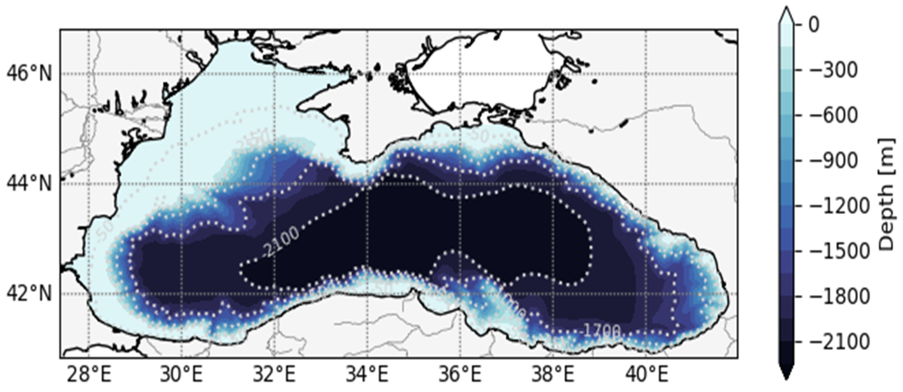
2.1. Atmospheric Forcing, Numerical Grid and Bathymetry
2.2. Hydrodynamical Model
2.3. Wave Model
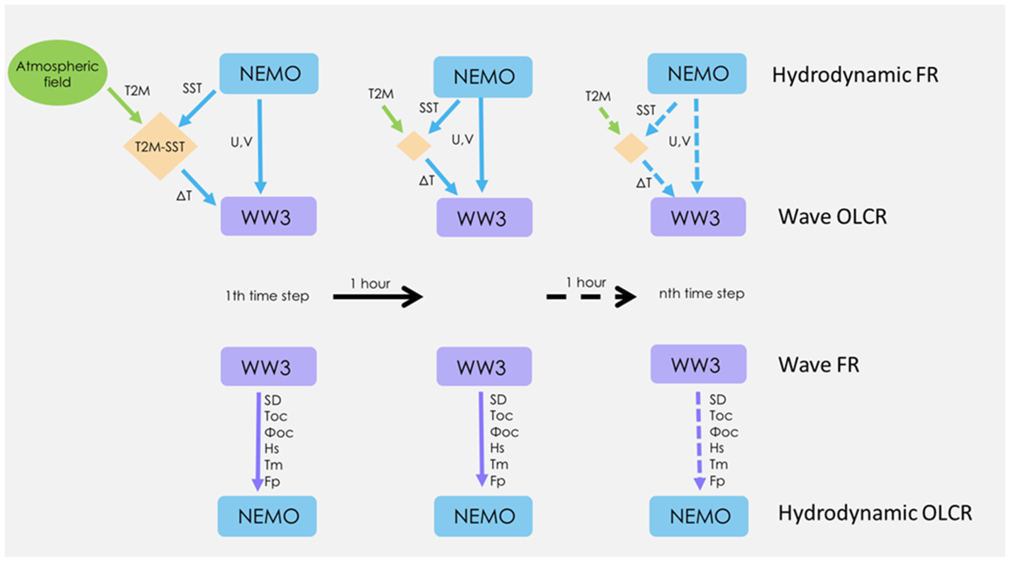
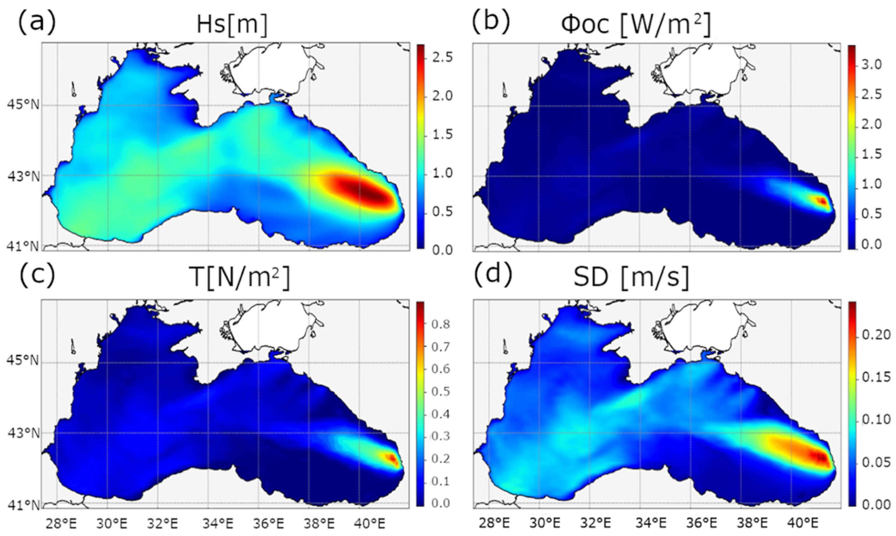
2.4. Coupling Strategy
- Sea-state dependent momentum flux;
- Stokes–Coriolis force, which requires a 3D-Stokes drift profile;
- Wave induced turbulence;
- Doppler effect and refraction due to currents;
- Effects of air stability on the growth rate of waves.
2.4.1. Sea-State Dependent Momentum Flux
2.4.2. Stokes–Coriolis Force and 3D-Stokes Drift Profile
2.4.3. Wave Induced Turbulence
2.4.4. Doppler Effect and Refraction Due to Currents
2.4.5. Effects of Air Stability on the Growth Rate of Waves
3. Numerical Experiments Design and Validation Strategy
Validation Strategy and Observational Data
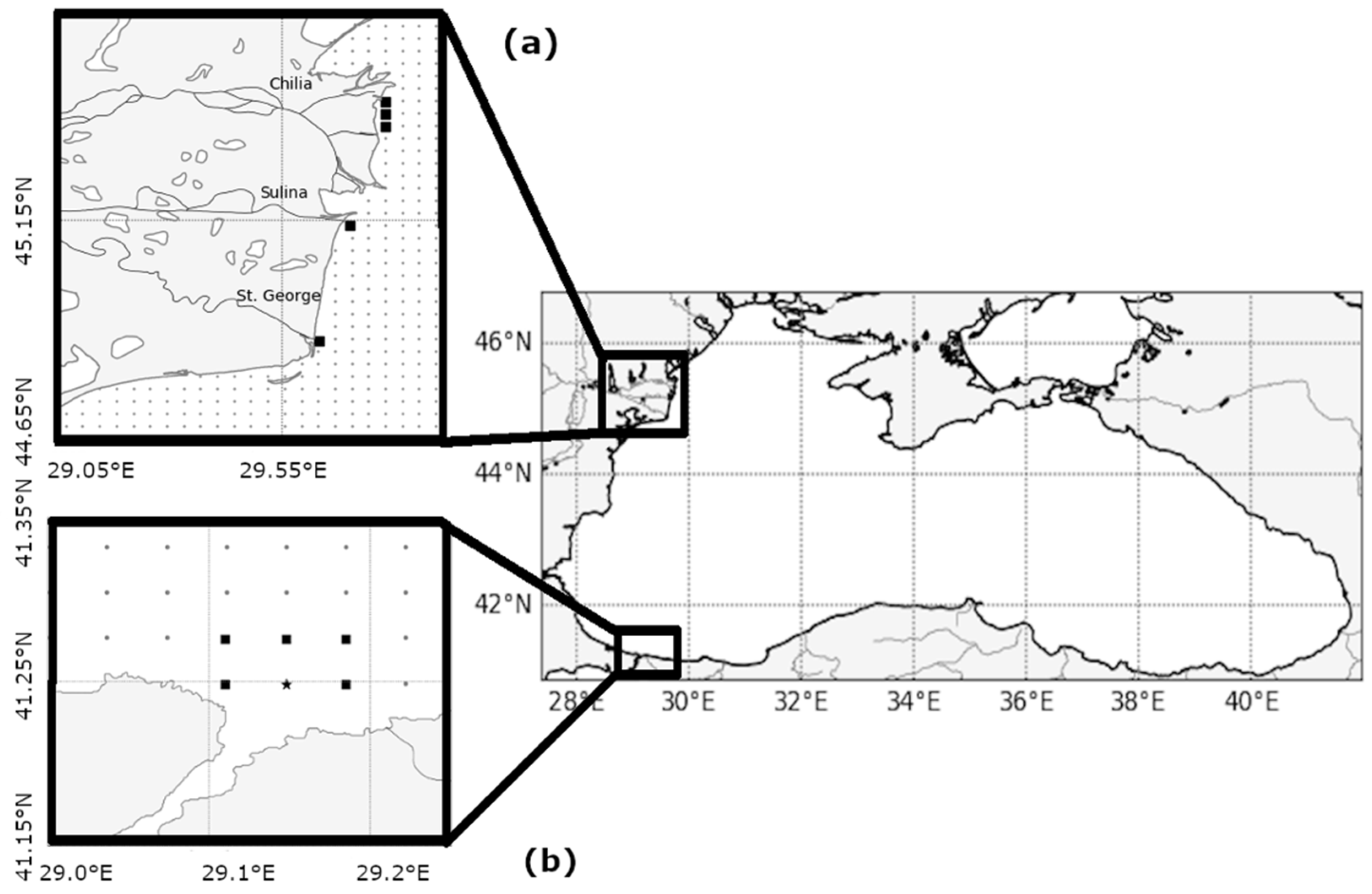
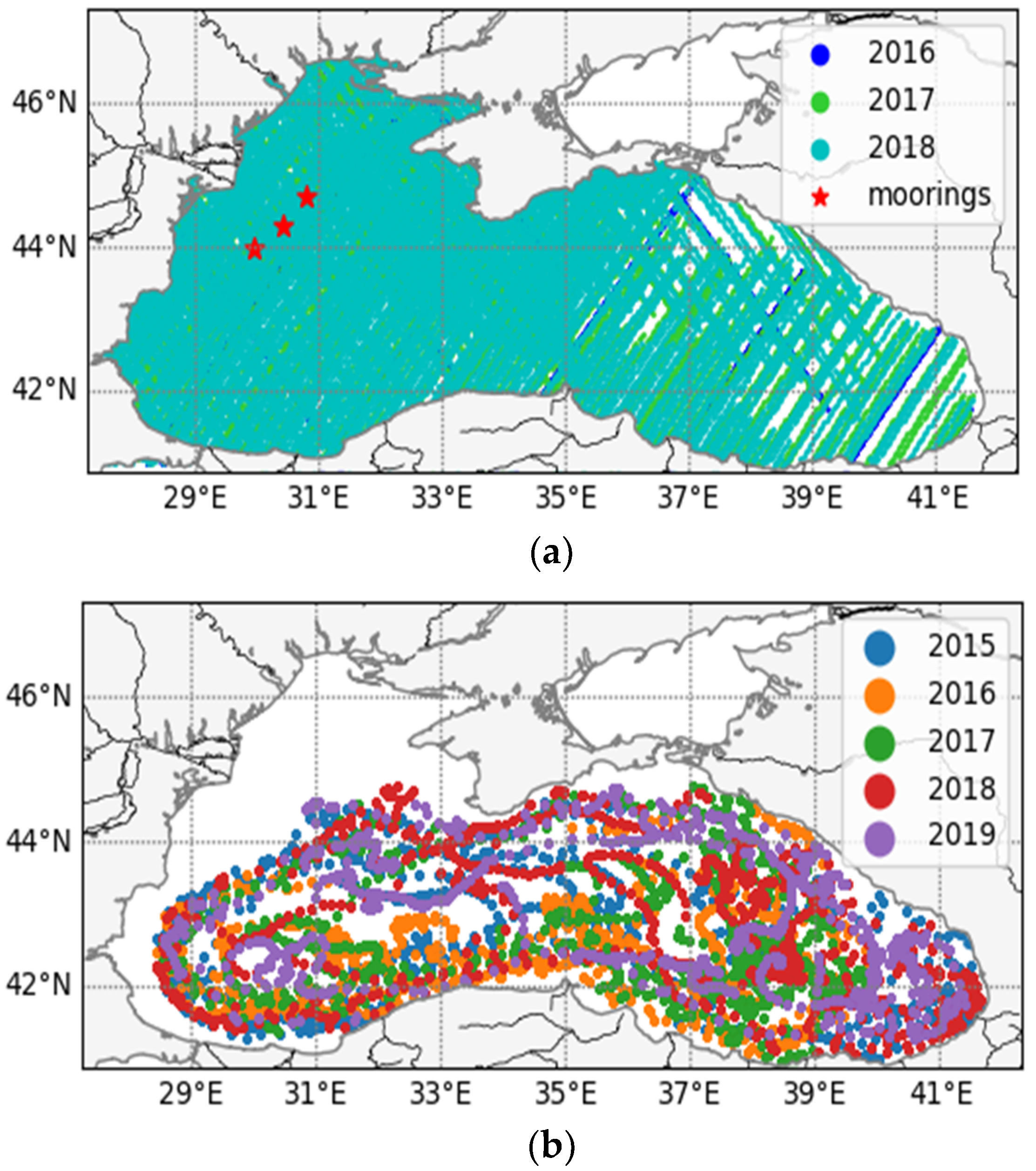
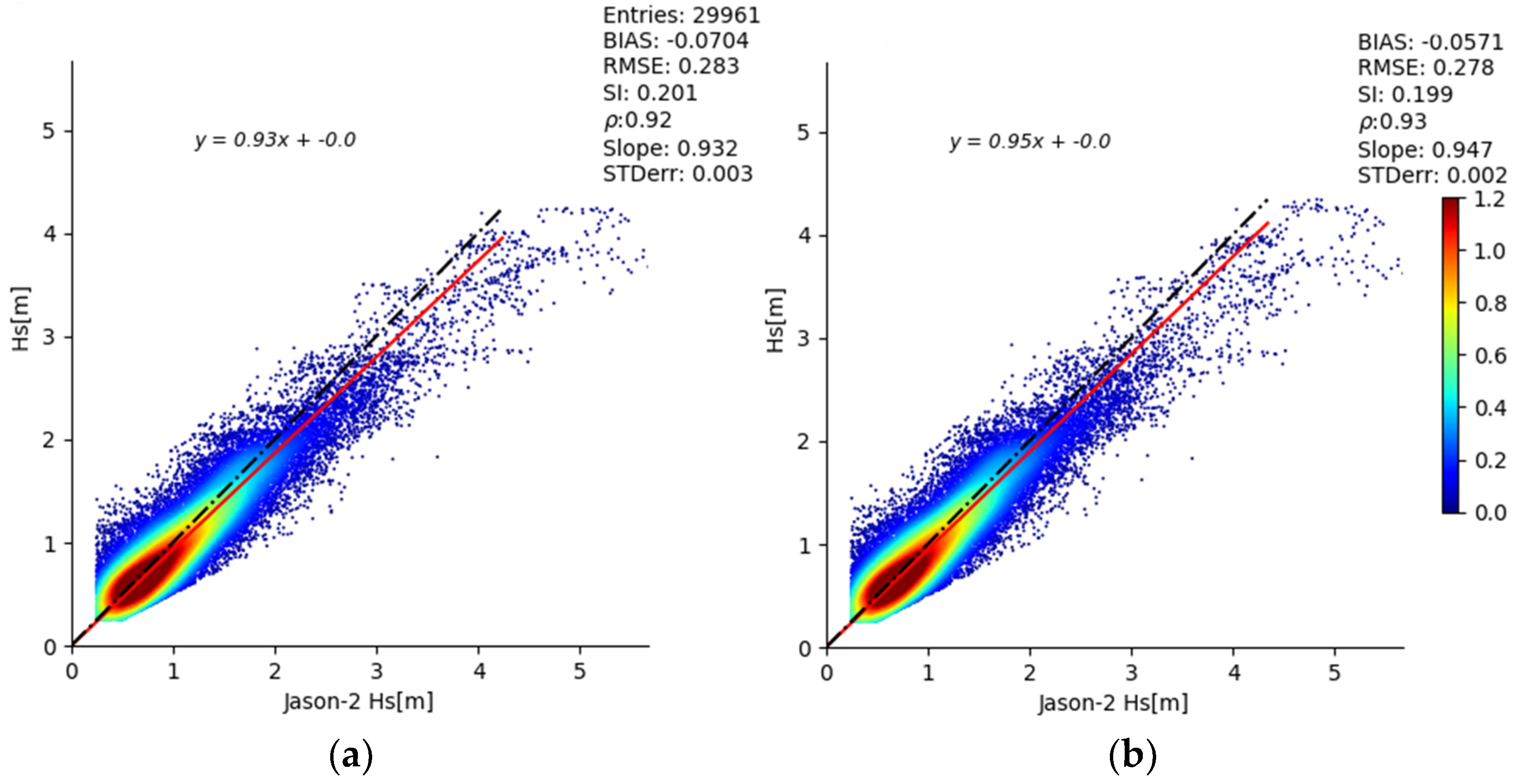
- Satellite: including Hs and Sea Surface Temperature (SST). Jason-2 (J2) along-track and quality-controlled altimetric measurements of Hs at 1 Hz sampling frequency (represented in Figure 5a), from the “Archiving, Validation and Interpretation of Satellite Oceanographic data” (AVISO+) have been used for the wave validation.
- SST data are provided by the CMEMS SST Thematic Assembly Center [101]. Nighttime L3 satellite data from different space missions are filtered according to quality check, bias-corrected, merged and provided at 1/16° of horizontal resolution. Dataset also provides an error estimate from the optimal interpolation. The operational maintenance of SST data is guaranteed by Consiglio Nazionale delle Ricerche—Istituto di Scienze Marine (CNR ISMAR, Venice, Italy).
- Argo: quality-controlled temperature and salinity in situ vertical profiles used in this work are provided by the CMEMS In Situ TAC [102]. The spatial distribution of almost 1400 Argo floats in the Black Sea basin over the period 2015–2019 is shown in Figure 5b. The operational maintenance of such data is coordinated by the Institute of Oceanology—Bulgarian Academy of Science (IO-BAS, Varna, Bulgaria).
4. Results and Discussion
4.1. Validation of Hydrodynamical Component
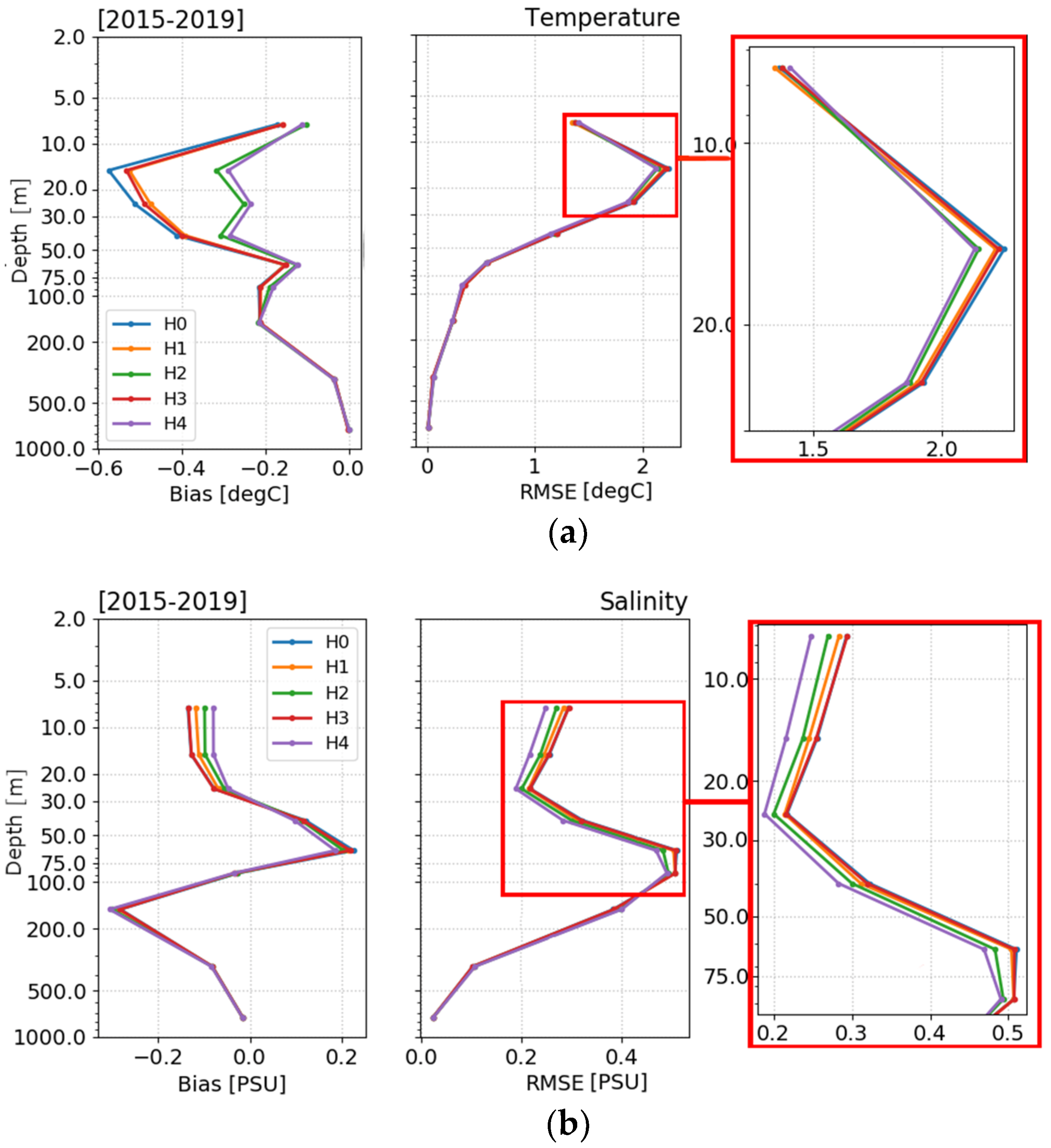
4.1.1. T/S Profiles
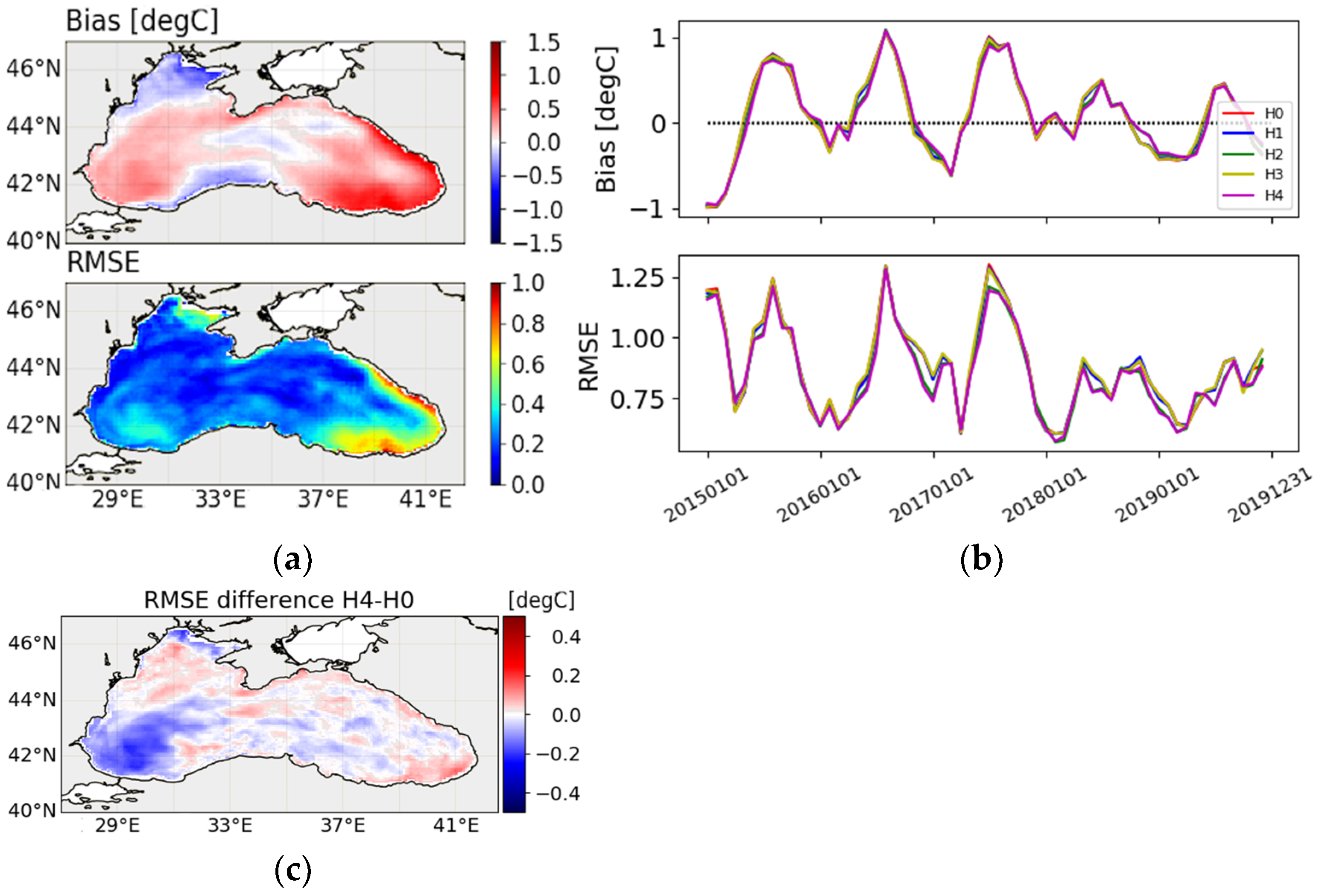
4.1.2. SST
4.1.3. Water Masses
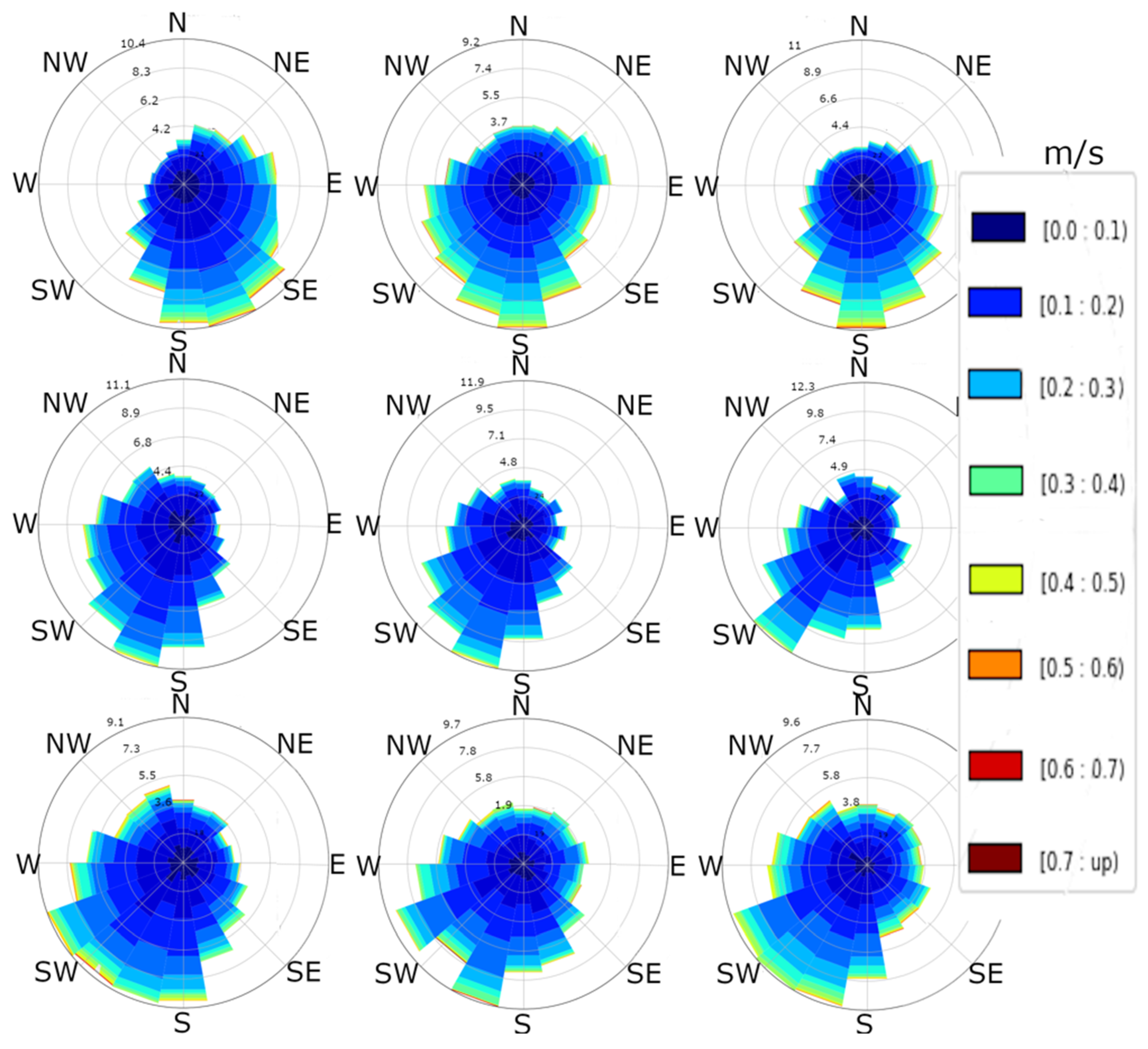
4.1.4. Currents
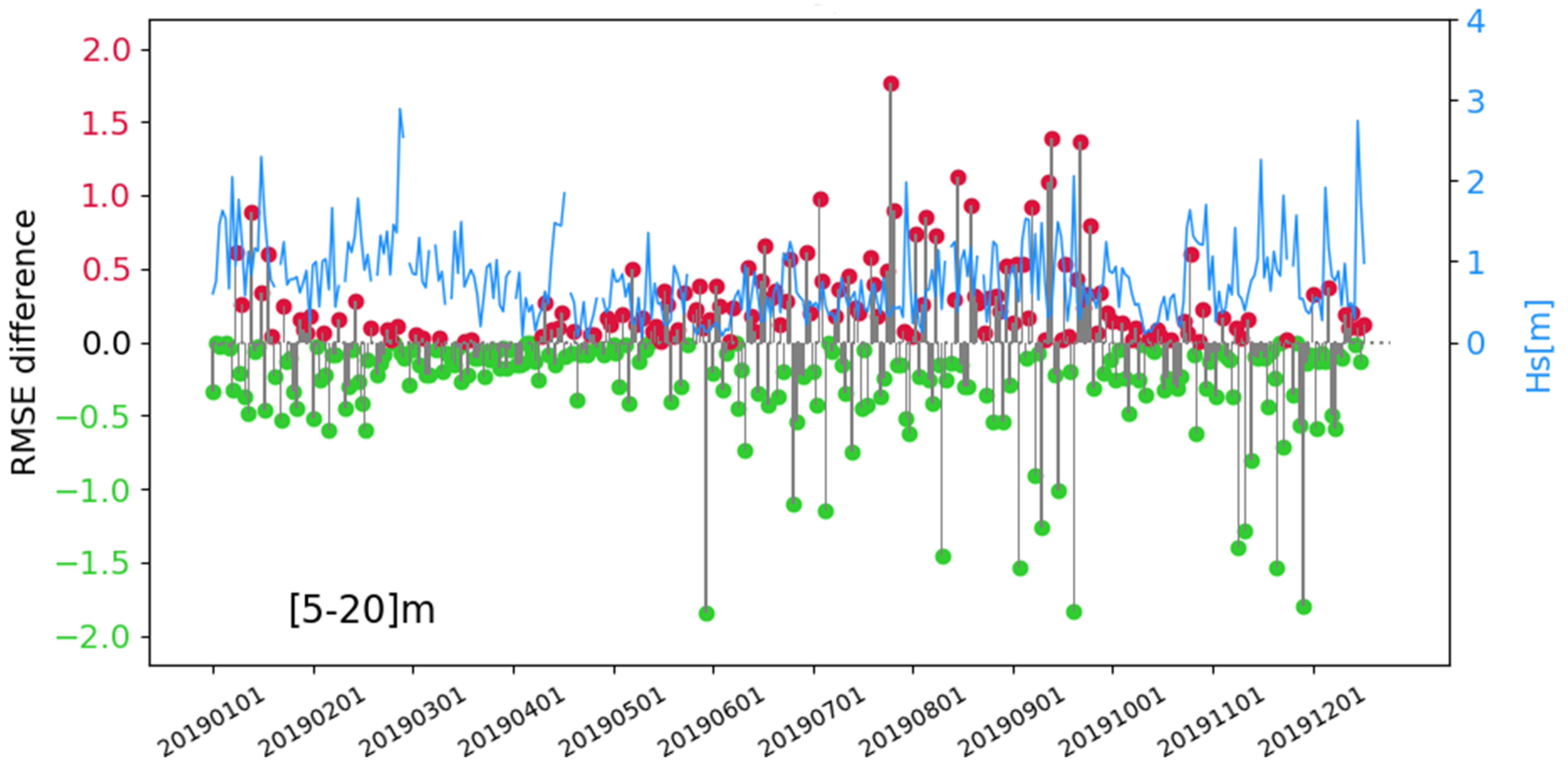
4.1.5. RMSE vs. Significant Wave Height
4.1.6. Validation for the Wave Component
5. Conclusions
Author Contributions
Funding
Institutional Review Board Statement
Informed Consent Statement
Conflicts of Interest
References
- Roland, A.; Ardhuin, F. On the developments of spectral wave models: Numerics and parameterizations for the coastal ocean. Ocean. Dyn. 2014, 64, 833–846. [Google Scholar] [CrossRef]
- Bolaños, R.; Tornfeldt Sørensen, J.V.; Benetazzo, A.; Carniel, S.; Sclavo, M. Modelling ocean currents in the northern Adriatic Sea. Cont. Shelf Res. 2014, 87, 54–72. [Google Scholar] [CrossRef]
- Longuet-Higgins, M.S.; Stewart, R.W. The changes in amplitude of short gravity waves on steady non-uniform currents. J. Fluid Mech. 1961, 10, 529–549. [Google Scholar] [CrossRef]
- Hsiao, S.C.; Chen, H.; Chen, W.B.; Chang, C.H.; Lin, L.Y. Quantifying the contribution of nonlinear interactions to storm tide simulations during a super typhoon event. Ocean. Eng. 2019, 194, 106661. [Google Scholar] [CrossRef]
- Hsiao, S.C.; Wu, H.L.; Chen, W.B.; Chang, C.H.; Lin, L.Y. On the Sensitivity of Typhoon Wave Simulations to Tidal Elevation and Current. J. Mar. Sc. Eng. 2020, 8, 731. [Google Scholar] [CrossRef]
- Janssen, P.A.E.M. Ocean wave effects on the daily cycle in SST. J. Geophys. Res. 2012, 117, C11. [Google Scholar] [CrossRef] [Green Version]
- Couvelard, X.; Lemarié, F.; Samson, G.; Redelsperger, J.L.; Ardhuin, F.; Benshila, R.; Madec, G. Development of a two-way-coupled ocean–wave model: Assessment on a global NEMO (v3. 6)–WW3 (v6. 02) coupled configuration. Geosci. Model Dev. 2020, 13, 3067–3090. [Google Scholar] [CrossRef]
- Lewis, H.W.; Castillo Sanchez, J.M.; Siddorn, J.; King, R.R.; Tonani, M.; Saulter, A.; Sykes, P.; Pequignet, A.C.; Weedon, G.P.; Palmer, T.; et al. Can wave coupling improve operational regional ocean forecasts for the north-west European Shelf? Ocean Sci. 2019, 15, 669–690. [Google Scholar] [CrossRef] [Green Version]
- Hasselmann, K. Wave-driven inertial oscillations. Geophys. Astrophys. Fluid Dyn. 1970, 1, 463–502. [Google Scholar] [CrossRef]
- McWilliams, J.C.; Restrepo, J.M.; Lane, E.M. An asymptotic theory for the interaction of waves and currents in coastal waters. J. Fluid Mech. 2004, 511, 135–178. [Google Scholar] [CrossRef]
- Craig, P.D.; Banner, M.L. Modeling Wave-Enhanced Turbulence in the Ocean Surface Layer. J. Phys. Oceanogr. 1994, 24, 2546–2559. [Google Scholar] [CrossRef] [Green Version]
- McWilliams, J.C.; Restrepo, J.M. The wave-driven ocean circulation. J. Phys. Oceanogr. 1991, 29, 2523–2540. [Google Scholar] [CrossRef]
- McWilliams, J.C.; Sullivan, P. Vertical mixing by Langmuir circulations. Spill Sci. Technol. Bull. 2000, 6, 225–237. [Google Scholar] [CrossRef]
- Mellor, G.; Blumberg, A. Wave Breaking and Ocean Surface Layer Thermal Response. J. Phys. Oceanogr. 2004, 34, 693–698. [Google Scholar] [CrossRef]
- Ardhuin, F.; Jenkins, A.D. On the Interaction of Surface Waves and Upper Ocean Turbulence. J. Phys. Oceanogr. 2006, 36, 551–557. [Google Scholar] [CrossRef]
- Huang, C.J.; Qiao, F.; Song, Z.; Ezer, T. Improving simulations of the upper ocean by inclusion of surface waves in the Mellor-Yamada turbulence scheme. J. Geophys. Res. 2011, 116. [Google Scholar] [CrossRef] [Green Version]
- Janssen, P.A.E.M.; Breivik, Ø.; Mogensen, K.; Vitart, F.; Balmaseda, M.; Bidlot, J.R.; Molteni, F. Air-sea interaction and surface waves. Eur. Cent. Medium-Range Weather. Forecast. 2013, 35. [Google Scholar] [CrossRef]
- Belcher, S.E.; Grant, A.L.; Hanley, K.E.; Fox-Kemper, B.; Van Roekel, L.; Sullivan, P.P.; Polton, J.A. A global perspective on Langmuir turbulence in the ocean surface boundary layer. Geophys. Res. Lett. 2012, 39. [Google Scholar] [CrossRef] [Green Version]
- Babanin, A.V.; Haus, B.H. On the existence of water turbulence induced by nonbreaking surface waves. J. Phys. Oceanogr. 2009, 39, 2675–2679. [Google Scholar] [CrossRef]
- Hackett, B.; Breivik, Ø.; Wettre, C. Forecasting the Drift of Objects and Substances in the Ocean. In Ocean Weather Forecasting; Springer: Berlin/Heidelberg, Germany, 2006; pp. 507–523. [Google Scholar]
- Breivik, Ø.; Allen, A.A. An operational search and rescue model for the Norwegian Sea and the North Sea. J. Mar. Syst. 2008, 69, 99–113. [Google Scholar] [CrossRef] [Green Version]
- Davidson, F.J.; Allen, A.; Brassington, G.B.; Breivik, Ø.; Daniel, P.; Kamachi, M.; Kaneko, H. Applications of GODAE ocean current forecasts to search and rescue and ship routing. Oceanography 2009, 22, 176–181. [Google Scholar] [CrossRef] [Green Version]
- Breivik, Ø.; Allen, A.A.; Maisondieu, C.; Olagnon, M. Advances in search and rescue at sea. Ocean Dyn. 2013, 63, 83–88. [Google Scholar] [CrossRef] [Green Version]
- Alari, V.; Staneva, J.; Breivik, Ø.; Bidlot, J.R.; Mogensen, K.; Janssen, P.A.E.M. Surface wave effects on water temperature in the Baltic Sea: Simulations with the coupled NEMO-WAM model. Ocean Dyn. 2016, 66, 917–930. [Google Scholar] [CrossRef]
- Staneva, J.; Alari, V.; Breivik, Ø.; Bidlot, J.R.; Mogensen, K. Effects of wave-induced forcing on a circulation model of the North Sea. Ocean Dyn. 2017, 67, 81–101. [Google Scholar] [CrossRef]
- Breivik, Ø.; Janssen, P.A.E.M.; Bidlot, J.R. Approximate Stokes Drift Profiles in Deep Water. J. Phys. Oceanogr. 2014, 44, 2433–2445. [Google Scholar] [CrossRef] [Green Version]
- Breivik, Ø.; Mogensen, K.; Bidlot, J.R.; Balmaseda, M.; Janssen, P.A.E.M. Surface wave effects in the NEMO ocean model: Forced and coupled experiments: Waves in NEMO. en. J. Geophys. Res. Oceans 2015, 120, 2973–2992. [Google Scholar] [CrossRef] [Green Version]
- Staneva, J.; Ricker, M.; Carrasco Alvarez, R.; Breivik, Ø.; Schrum, C. Effects of wave-induced processes in a coupled Wave–Ocean model on particle transport simulations. Water 2021, 13, 415. [Google Scholar] [CrossRef]
- Clementi, E.; Oddo, P.; Drudi, M.; Pinardi, N.; Korres, G.; Grandi, A. Coupling hydrodynamic and wave models: First step and sensitivity experiments in the Mediterranean Sea. Ocean Dyn. 2017, 67, 1293–1312. [Google Scholar] [CrossRef] [Green Version]
- Bruciaferri, D.; Tonani, M.; Lewis, H.W.; Siddorn, J.R.; Saulter, A.; Castillo, J.M.; McConnell, N. The impact of ocean-wave coupling on the upper ocean circulation during storm events. J. Geophys. Res. Ocean. 2021, e2021JC017343. [Google Scholar] [CrossRef]
- Stanev, E.V. Black Sea dynamics. Oceanography 2005, 18, 56. [Google Scholar] [CrossRef] [Green Version]
- Ivanov, V.A.; Belokopytov, V.N. Oceanography of the Black Sea; National Academy of Science of Ukraine, Marine Hydrophysical Institute: Sevastopol, Russia, 2013; 210p. [Google Scholar]
- Özsoy, E.; Di Iorio Dm Gregg, M.C.; Backhaus, J.O. Mixing in the Bosphorus Strait and the Black Sea continental shelf: Observations and a model of the dense water outflow. J. Mar. Syst. 2001, 31, 99–135. [Google Scholar] [CrossRef]
- Mikhailov, V.N.; Mikhailova, M.V. River Mouths in the Black Sea Environment; Kostianoy, A.G., Kosarev, A.N., Eds.; Springer: Berlin/Heidelberg, Germany, 2008; pp. 91–133. [Google Scholar] [CrossRef]
- Kara, A.; Birol, J.; Wallcraft, A.; Hurlburt, H.; Stanev, E.V. Air–sea fluxes and river discharges in the Black Sea with a focus on the Danube and Bosphorus. J. Mar. Syst. 2008, 74, 74–95. [Google Scholar] [CrossRef]
- Miladinova, S.; Stips, A.; Macias Moy, D.; Garcia-Gorriz, E. Pathways and mixing of the north western river waters in the Black Sea. Estuar. Coast. Shelf Sci. 2020, 236, 106630. [Google Scholar] [CrossRef]
- Stanev, E.V. On the mechanisms of the Black Sea circulation. Earth-Sci. Rev. 1990, 28, 285–319. [Google Scholar] [CrossRef]
- Oguz, T.; Malanotte-Rizzoli, P. Seasonal variability of wind and thermohaline-driven circulation in the Black Sea: Modeling studies. J. Geophys. Res. Oceans 1996, 101, 16551–16569. [Google Scholar] [CrossRef]
- Lima, L.; Ciliberti, S.A.; Aydogdu, A.; Masina, S.; Escudier, R.; Cipollone, A.; Azevedo, D.; Causio, S.; Peneva, E.; Lecci, R.; et al. Climate signals in the Black Sea from a multidecadal eddy-resolving reanalysis. Front. Mar. Sci. 2021, in press. [Google Scholar] [CrossRef]
- Gunduz, M.; Özsoy, E.; Hordoir, R. A model of Black Sea circulation with strait exchange (2008–2018). Geosci. Model Dev. 2020, 13, 121–138. [Google Scholar] [CrossRef] [Green Version]
- Sadighrad, E.; Fach, B.A.; Arkin, S.S.; Salihoğlu, B.; Hüsrevoğlu, S. Mesoscale eddies in the Black Sea: Characteristics and kinematic, properties in a high-resolution ocean model. J. Mar. Syst. 2021, 2021, 103613. [Google Scholar] [CrossRef]
- Bruciaferri, D.; Shapiro, G.; Stanichny, S.; Zatsepin, A.; Ezer, T.; Wobus, F.; Hilton, D. The development of a 3D computational mesh to improve the representation of dynamic processes: The Black Sea test case. Ocean Model. 2020, 146, 101534. [Google Scholar] [CrossRef]
- Staneva, J.V.; Dietrich, D.E.; Stanev, E.V.; Bowman, M.J. Rim current and coastal eddy mechanisms in an eddy-resolving Black Sea general circulation model. J. Mar. Syst. 2001, 31, 137–157. [Google Scholar] [CrossRef] [Green Version]
- Oguz, T.; Besiktepe, S. Observations on the Rim Current structure, CIW formation and transport in the western Black Sea. Deep. Sea Res. Part I Oceanogr. Res. Pap. 1999, 46, 1733–1753. [Google Scholar] [CrossRef]
- Stanev, E.; Peneva, E.; Chtirkova, B. Climate Change and Regional Ocean Water Mass Disappearance: Case of the Black Sea. J. Geophys. Res. Ocean. 2019, 124, 4803–4819. [Google Scholar] [CrossRef]
- Murray, J.W.; Jannasch, H.W.; Honjo, S.; Anderson, R.F.; Reeburgh, W.S.; Top, Z.; Friederich, G.E.; Codispoti, L.A.; Izdar, E. Unexpected changes in the oxic/anoxic interface in the Black Sea. Nature 1989, 338, 411–413. [Google Scholar] [CrossRef]
- Rusu, L.; Bernardino, M.; Guedes Soares, C. Wind and wave modelling in the Black Sea. J. Oper. Oceanogr. 2014, 7, 5–20. [Google Scholar] [CrossRef] [Green Version]
- Belokopytov, V.N.; Kudryavtseva GFLipchenko, M.M. Atmospheric pressure and wind over the Black Sea (1961–1990). Trudy UkrNIGMI 1998, 246, 174–181. (In Russian) [Google Scholar]
- Schrum, C.; Staneva, J.; Stanev, E.; Özsoy, E. Air–sea exchange in the Black Sea estimated from atmospheric analysis for the period 1979–1993. J. Mar. Syst. 2001, 31, 3–19. [Google Scholar] [CrossRef] [Green Version]
- Efimov, V.V.; Timofeev, N.A. Heat Balance Studies of the Black Sea and the Sea of Azov; VNIIGMI-MCD: Obninsk, Russia, 1990; Available online: https://scholar.google.com.hk/scholar?hl=zh-CN&as_sdt=0%2C5&q=Heat+balance+studies+of+the+Black+Sea+and+the+Sea+of+Azov&btnG= (accessed on 18 August 2021).
- Zecchetto, S.; De Biasio, F. Sea Surface Winds over the Mediterranean Basin from Satellite Data (2000–04): Meso- and Local-Scale Features on Annual and Seasonal Time Scales. J. Appl. Meteorol. Climatol. 2007, 46, 814–827. [Google Scholar] [CrossRef]
- Munk, W.H. Wind stress on water: An hypothesis. Q. J. R. Meteorol. Soc. 1955, 81, 320–332. [Google Scholar] [CrossRef]
- Pierson, W.J., Jr.; Moskowitz, L. A proposed spectral form for fully developed wind seas based on the similarity theory of SA Kitaigorodskii. J. Geophys. Res. 1964, 69, 5181–5190. [Google Scholar] [CrossRef]
- Rzheplinkskij, G.V. Wind and Wave Atlas of the Black Sea; Gidrometeoizdat: St. Petersburg, Russia, 1969; Available online: https://www.google.com.hk/search?newwindow=1&source=univ&tbm=isch&q=54.%09Rzheplinkskij,+G.V.+Wind+and+Wave+Atlas+of+the+Black+Sea&sa=X&ved=2ahUKEwii76fdkLzyAhWSMd4KHZJ3D9QQjJkEegQIIRAC&biw=1280&bih=539 (accessed on 18 August 2021). (In Russian)
- Simonov, A.I.; Altman, E.N. Hydrometeorology and Hydrochemistry of the USSR Seas; The Black Sea; Gidrometeoizdat: St. Petersburg, Russia, 1991; Volume IV, Available online: https://scholar.google.com.hk/scholar?cluster=399150530370965865&hl=zh-CN&as_sdt=2005&sciodt=0,5 (accessed on 18 August 2021).
- Polonsky, A.B.; Popov, Y.I.; Conditions for Formation of the Cold Intermediate Layer in the Black Sea. MGI Sevastapol 2011. Available online: https://scholar.google.com.hk/scholar?hl=zh-CN&as_sdt=0%2C5&q=Conditions+for+Formation+of+the+Cold+Intermediate+Layer+in+the+Black+Sea&btnG= (accessed on 18 August 2021). (In Russian).
- Arkhipkin, V.S.; Gippius, F.N.; Koltermann, K.P.; Surkova, G.V. Wind waves in the Black Sea: Results of a hindcast study. Nat. Hazards Earth Syst. Sci. 2014, 14, 2883. [Google Scholar] [CrossRef] [Green Version]
- Law Chune, S.; Aouf, L. Wave effects in global ocean modelling: Parametrizations vs. forcing from a wave model. Ocean Dynam. 2018, 68, 1739–1758. [Google Scholar] [CrossRef]
- Owens, R.G.; Hewson, T. ECMWF Forecast User Guide. ECMWF Read. 2018. [Google Scholar] [CrossRef]
- Adler, R.F.; Huffman, G.J.; Chang, A.; Ferraro, R.; Xie, P.; Janowiak, J.; Rudolf, B.; Schneider, U.; Curtis, S.; Bolvin, D.; et al. The Version 2 Global Precipitation Climatology Project (GPCP) Monthly Precipitation Analysis (1979-Present). J. Hydrometeor. 2003, 4, 1147–1167. [Google Scholar] [CrossRef]
- Huffman, G.J.; Adler, R.F.; Bolvin, D.T.; Gu, G. Improving the Global Precipitation Record: GPCP Version 2.1. Geophys. Res. Lett. 2009, 36, L17808. [Google Scholar] [CrossRef] [Green Version]
- Weatherall, P.; Marks, K.M.; Jakobsson, M.; Schmitt, T.; Tani, S.; Arndt, J.E.; Wigley, R. A new digital bathymetric model of the world’s oceans. Earth Space Sci. 2015, 2, 331–345. [Google Scholar] [CrossRef]
- Gürses, O.; Aydōgdu, A.; Pinardi, N.; Özsoy, E. A finite element modeling study of the Turkish Straits System. In The Sea of Marmara—Marine Biodiversity, Fisheries, Conservations and Governance; TUDAV: Istambul, Turkey, 2016; pp. 169–184. [Google Scholar]
- Gürses, Ö. Dynamics of the Turkish Straits System—A Numerical Study with a Finite Element Ocean Model Based on an Unstructured Grid Approach. Ph.D. Thesis, Middle East Technical University, Ankara, Turkey, 2016. [Google Scholar]
- Madec, G.; NEMO System Team. Scientific Notes of Climate Modelling Center, User manual. NEMO Ocean Engine 2017. [Google Scholar] [CrossRef]
- Myroshnychenko, V.; Simoncelli, S.; Troupin, C. SeaDataCloud Temperature and Salinity Climatology for the Black Sea (Version 1). Prod. Inf. Doc. 2019. [Google Scholar] [CrossRef]
- Pettenuzzo, D.; Large, W.G.; Pinardi, N. On the corrections of ERA-40 surface flux products consistent with the Mediterranean heat and water budgets and the connection between basin surface total heat flux and NAO. J. Geophys. Res. Oceans 2010, 115. [Google Scholar] [CrossRef]
- Tonani, M.; Pinardi, N.; Dobricic, S.; Pujol, I.; Fratianni, C. A high-resolution free-surface model of the Mediterranean Sea. Ocean Sci. Discuss. 2008, 4, 213–244. [Google Scholar] [CrossRef] [Green Version]
- Oddo, P.; Adani, M.; Pinardi, N.; Fratianni, C.; Tonani, M.; Pettenuzzo, D. A nested Atlantic-Mediterranean Sea general circulation model for operational forecasting. Ocean Sci. 2009, 5, 461–473. [Google Scholar] [CrossRef] [Green Version]
- Ludwig, W.; Dumont, E.; Meybeck, M.; Heussner, S. River discharges of water and nutrients to the Mediterranean and Black Sea: Major drivers for ecosystem changes during past and future decades? Prog. Oceanogr. 2009, 80, 199–217. [Google Scholar] [CrossRef]
- Panin, N.; Jipa, D. Danube River sediment input and its interaction with the north-western Black Sea. Estuar. Coast. Shelf Sci. 2002, 54, 551–562. [Google Scholar] [CrossRef]
- Stanev, E.; Beckers, J.M. Barotropic and baroclinic oscillations in strongly stratified ocean basins: Numerical study of the Black Sea. J. Mar. Syst. 1999, 19, 65–112. [Google Scholar] [CrossRef]
- Peneva, E.L.; Stanev, E.; Belokopytov, V.; Le Traon, P.Y. Water transport in the Bosphorus Straits estimated from hydro-meteorologycal and altimeter data: Seasonal to decadal variability. J. Mar. Sys. 2001, 31, 21–35. [Google Scholar] [CrossRef]
- Aydogdu, A.; Pinardi, N.; Özsoy, E.; Danabasoglu, G.; Gürses, O.; Karspeck, A. Circulation of the Turkish Straits System under interannual atmospheric forcing. Ocean Sci. 2018, 14, 999–1019. [Google Scholar] [CrossRef] [Green Version]
- Causio, S.; Ciliberti, S.A.; Clementi, E.; Coppini, G.; Lionello, P. A Modeling Approach for the Assessment of Wave-Currents Interaction in the Black Sea. Available online: https://zenodo.org/record/5184753#.YR3VVt8RU2w (accessed on 18 August 2021).
- Tolman, H.L. User manual and system documentation of WAVEWATCH III TM version 3.14. Tech. Note MMAB Contrib. 2009, 276, 220. [Google Scholar]
- Günther, H.; Hasselmann, S.; Janssen, P.A.E.M. The WAM Model Cycle 4, User Manual; Dtsch: Klimarechenzentrum, Germany, 1992. No. DKRZ-TR--4 (REV. ED.). Available online: https://www.dkrz.de/mms/pdf/reports/ReportNo.04.pdf (accessed on 18 August 2021).
- Ardhuin, F.; Rogers, E.; Babanin, A.V.; Filipot, J.F.; Magne, R.; Roland, A.; Collard, F. Semiempirical dissipation source functions for ocean waves. Part I: Definition, calibration, and validation. J. Phys. Oceanogr. 2010, 40, 1917–1941. [Google Scholar] [CrossRef] [Green Version]
- Janssen, P.A.E.M. Quasi-linear Theory of Wind-Wave Generation Applied to Wave Forecasting. J. Phys. Oceanogr. 1998, 21, 1631–1642. [Google Scholar] [CrossRef] [Green Version]
- Chalikov, D.V.; Yu Belevich, M. One-dimensional theory of the wave boundary layer. Bound. Layer Meteorol. 1993, 63, 65–96. [Google Scholar] [CrossRef]
- Bidlot, J.; Abdalla, S.; Janssen, P.A.E.M. A revised formulation for ocean wave dissipation in CY25R1. Intern. Memo. Res. Department ECMWF 2005. [Google Scholar] [CrossRef]
- Bidlot, J.R. Intercomparison of operational wave forecasting systems against buoys: Data from ECMWF, MetOce, FNMOC, NCEP, DWD, BoM, SHOM and JMA, September 2008 to November 2008. In Joint WMO-IOC Technical Commission for Oceanography and Marine Meteorology; World Meteorological Organization: Geneva, Switzerland, 2008. [Google Scholar]
- Hasselmann, S.; Hasselmann, K.; Allender, J.K.; Barnett, T.P. Computations and parameterizations of the nonlinear energy transfer in a gravity-wave specturm. Part II: Parameterizations of the nonlinear energy transfer for application in wave models. J. Phys. Oceanogr. 1985, 15, 1378–1391. [Google Scholar] [CrossRef] [Green Version]
- Hasselmann, D.; Bösenberg, J.; Dunckel, M.; Richter, K.; Grünewald, M.; Carlson, C. Measurements of wave-induced pressure over surface gravity waves. In Wave Dynamics and Radio Probing of the Ocean Surface; Springer: Boston, MA, USA, 1986; pp. 353–368. [Google Scholar]
- Wu, L.; Staneva, J.; Breivik, Ø.; Rutgersson, A.; Nurser, A.G.; Clementi, E.; Madec, G. Wave effects on coastal upwelling and water level. Ocean Mod. 2019, 140, 101405. [Google Scholar] [CrossRef]
- Saetra, Ø.; Albretsen, J.; Janssen, P.A. Sea-state-dependent momentum fluxes for ocean modeling. J. Phys. Oceanogr. 2007, 37, 2714–2725. [Google Scholar] [CrossRef]
- Charnock, H. Wind stress on a water surface. Q. J. R. Meteorol. Soc. 1955, 81, 639–640. [Google Scholar] [CrossRef]
- Janssen, P.A. Wave-induced stress and the drag of air flow over sea waves. J. Phys. Oceanogr. 1989, 19, 745–754. [Google Scholar] [CrossRef] [Green Version]
- Taylor, P.K.; Yelland, M.J. The dependence of sea surface roughness on the height and steepness of the waves. J. Phys. Oceanogr. 2001, 31, 572–590. [Google Scholar] [CrossRef] [Green Version]
- Oost, W.A.; Komen, G.J.; Jacobs CM, J.; Van Oort, C. New evidence for a relation between wind stress and wave age from measurements during ASGAMAGE. Bound. Layer Meteorol. 2002, 103, 409–438. [Google Scholar] [CrossRef]
- Weber, J.E.H.; Broström, G.; Saetra, Ø. Eulerian versus Lagrangian approaches to the wave-induced transport in the upper ocean. J. Phys. Oceanogr. 2006, 36, 2106–2118. [Google Scholar] [CrossRef]
- Polton, J.A.; Lewis, D.M.; Belcher, S.E. The Role of Wave-Induced Coriolis–Stokes Forcing on the Wind-Driven Mixed Layer. J. Phys. Oceanogr. 2005, 35, 444–457. [Google Scholar] [CrossRef]
- Skyllingstad, E.D.; Denbo, D.W. An ocean large-eddy simulation of Langmuir circulations and convection in the surface mixed layer. J. Geophys. Res. Oceans 1995, 100, 8501–8522. [Google Scholar] [CrossRef]
- Carniel, S.; Sclavo, M.; Kantha, L.H.; Clayson, C.A. Langmuir cells and mixing in the upper ocean. Il Nuovo Cim. 2005, 28, 33–54. [Google Scholar]
- Polton, J.A.; Belcher, S.E. Langmuir turbulence and deeply penetrating jets in an unstratified mixed layer. J. Geophys. Res. Oceans 2007, 112. [Google Scholar] [CrossRef] [Green Version]
- Tamura, H.; Miyazawa, Y.; Oey, L.-Y. The Stokes drift and wave induced-mass flux in the North Pacific. J. Geophys. Res. Oceans 2012, 117. [Google Scholar] [CrossRef] [Green Version]
- Bennis, A.C.; Ardhuin, F. Comments on “The depth-dependent current and wave interaction equations: A revision”. J. Phys. Oceanogr 2011, 41, 2008–2012. [Google Scholar] [CrossRef] [Green Version]
- Tolman, H.L. Validation of WAVEWATCH III Version 1.15 for a Global Domain. Technical Report. NOAA/NWS/NCEP/OMB 2002, 213, 33. [Google Scholar]
- Kahma, K.K.; Calkoen, C.H. Reconciling Discrepancies in the Observed Growth of Wind-generated Waves. J. Phys. Oceanogr. 1992, 22, 1389–1405. [Google Scholar] [CrossRef] [Green Version]
- Hernandez, F.; Blockley, E.; Brassington, G.B.; Davidson, F.; Divakaran, P.; Drévillon, M.; Zhang, A. Recent progress in performance evaluations and near real-time assessment of operational ocean products. J. Phys. Oceanogr 2015, 8 (Suppl. 2), S221–S238. [Google Scholar] [CrossRef]
- Buongiorno Nardelli, B.; Tronconi, C.; Pisano, A.; Santoleri, R. High and Ultra-High resolution processing of satellite Sea Surface Temperature data over Southern European Seas in the framework of MyOcean project. Remote Sens. Environ. 2013, 129, 1–16. [Google Scholar] [CrossRef]
- Copernicus Marine In Situ TAC. Copernicus Marine In Situ TAC quality Information Document for Near Real Time. Situ Products (QUID SQO) 2021. [Google Scholar] [CrossRef]
- Venables, W.N.; Ripley, B.D. Random and mixed effects. In Modern Applied Statistics with S; Springer: New York, NY, USA, 2002; pp. 271–300. [Google Scholar]
- Cavaleri, L.; Fox-Kemper, B.; Hemer, M. Wind Waves in the Coupled Climate System. Bull. Am. Meteorol. Soc. 2012, 93, 1651–1661. [Google Scholar] [CrossRef]
- Fan, Y.; Griffes, S.M. Impacts of Parameterized Langmuir Turbulence and Nonbreaking Wave Mixing in Global Climate Simulations. J. Clim. 2014, 27, 4752–4775. [Google Scholar] [CrossRef]


| ID | Experiment | Description |
|---|---|---|
| H0 | NEMO standalone | ΝΕΜO free-run. The hydrodynamic model is a standalone model |
| H1 | NEMO forced via SD | NEMO single field-forced experiment. It uses Stokes Drift at the surface from the WM. Stokes–Coriolis Force (SCF) based on the 3-D reconstruction of the Stokes velocity profile has been computed by the HM |
| H2 | NEMO forced via τoc | NEMO single field-forced experiment. It uses sea-state dependent momentum flux (τoc) from WM |
| H3 | NEMO forced via Φoc | NEMO single field-forced experiment. It uses wave-induced vertical mixing (Φoc) from WM |
| H4 | NEMO forced via SD + τoc + Φoc | ΝΕΜO fully-forced experiment. Ιt uses SCF, τoc and Φoc |
| W0 | WW3 standalone | WW3 free-run. The wave model is a standalone model |
| W1 | WW3 forced via u, v | WW3 single field-forced experiment. It uses currents from the HM |
| W2 | WW3 forced via ΔT | WW3 single field-forced experiment. It uses ΔΤ from the HM and atmospheric forcings |
| W3 | WW3 forced via u, v + ΔT | WW3 fully-forced experiment. It uses currents and ΔΤ |
| Dataset | Producer | Variable | Product Name | DOI/URL/Reference |
|---|---|---|---|---|
| SATELLITE | AVISO+ | Hs | Jason-2 Geophysical Data Records (GDR) from precise orbit | https://www.aviso.altimetry.fr/en/data/products/wind/wave-products/gdr-ogdr-osdr-ra2-wwv.html#c6705 (accessed on 1 July 2021) |
| ARGO | CMEMS | T and S vertical profiles | INSITU_GLO_TS_REP_ OBSERVATIONS_013_001_b | [102] |
| SATELLITE | CMEMS | SST | SST_BLK_SST_L4_NRT_ OBSERVATIONS_010_006 | [101] |
| Mooring EUXRo (01, 02, 03) | CMEMS | Currents speed and direction | INSITU_GLO_TS_REP_ OBSERVATIONS_013_001_b | [102] |
| Metric | Experiment | Year 2015 | Year 2016 | Year 2017 | Year 2018 | Year 2019 | Years 2015–2019 |
|---|---|---|---|---|---|---|---|
| BIAS | H0 | −0.63 | −0.43 | −0.15 | −0.05 | −0.17 | −0.29 ± 0.075 |
| H1 | −0.61 | −0.41 | −0.14 | −0.03 | −0.16 | −0.27 ± 0.075 | |
| H2 | −0.54 | −0.31 | −0.07 | 0.04 | −0.09 | −0.19 ± 0.071 | |
| H3 | −0.61 | −0.41 | −0.13 | −0.05 | −0.17 | −0.27 ± 0.077 | |
| H4 | −0.55 | −0.28 | −0.04 | 0.04 | −0.1 | −0.18 ± 0.073 | |
| RMSE | H0 | 1.22 | 1.04 | 0.86 | 0.95 | 0.88 | 0.99 ± 0.034 |
| H1 | 1.2 | 1.02 | 0.86 | 0.94 | 0.89 | 0.98 ± 0.034 | |
| H2 | 1.19 | 0.91 | 0.88 | 0.98 | 0.89 | 0.97 ± 0.03 | |
| H3 | 1.2 | 1.03 | 0.87 | 0.95 | 0.89 | 0.99 ± 0.032 | |
| H4 | 1.18 | 0.91 | 0.88 | 0.97 | 0.88 | 0.96 ± 0.029 | |
| No observations | 149,928 | 169,312 | 161,799 | 151,030 | 130,869 | 762,938 |
| Metric | Experiment | Year 2015 | Year 2016 | Year 2017 | Year 2018 | Year 2019 | Years 2015–2019 |
|---|---|---|---|---|---|---|---|
| BIAS | H0 | −0.09 | −0.15 | −0.06 | 0.08 | −0.03 | −0.05 ± 0.212 |
| H1 | −0.09 | −0.14 | −0.06 | 0.08 | −0.02 | −0.05 ± 0.208 | |
| H2 | −0.08 | −0.14 | −0.06 | 0.07 | −0.01 | −0.04 ± 0.207 | |
| H3 | −0.09 | −0.15 | −0.07 | 0.08 | −0.03 | −0.05 ± 0.205 | |
| H4 | −0.09 | −0.14 | −0.08 | 0.08 | −0.01 | −0.04 ± 0.208 | |
| RMSE | H0 | 0.29 | 0.33 | 0.3 | 0.31 | 0.39 | 0.32 ± 0.128 |
| H1 | 0.29 | 0.33 | 0.29 | 0.3 | 0.38 | 0.32 ± 0.122 | |
| H2 | 0.29 | 0.32 | 0.28 | 0.3 | 0.37 | 0.31 ± 0.113 | |
| H3 | 0.29 | 0.33 | 0.3 | 0.31 | 0.38 | 0.32 ± 0.12 | |
| H4 | 0.28 | 0.31 | 0.27 | 0.29 | 0.35 | 0.3 ± 0.115 | |
| No observations | 149,928 | 169,312 | 161,799 | 151,030 | 130,869 | 762,938 |
| Experiment | Metric | Variable | DJF | MAM | JJA | SON |
|---|---|---|---|---|---|---|
| H0 | BIAS | Salinity [PSU] | −0.06 ± 0.058 | −0.09 ± 0.116 | 0 ± 0.088 | −0.03 ± 0.065 |
| Temperature {°C} | −0.25 ± 0.245 | −0.33 ± 0.179 | −0.29 ± 0.243 | −0.28 ± 0.255 | ||
| RMSE | Salinity [PSU] | 0.3 ± 0.01 | 0.31 ± 0.035 | 0.31 ± 0.023 | 0.33 ± 0.08 | |
| Temperature {°C} | 0.66 ± 0.167 | 0.60 ± 0.123 | 1.17 ± 0.11 | 1.23 ± 0.138 | ||
| H4 | BIAS | Salinity [PSU] | −0.06 ± 0.56 | −0.08 ± 0.107 | −0.01 ± 0.085 | −0.02 ± 0.06 |
| Temperature {°C} | −0.19 ± 0.242 | −0.28 ± 0.176 | −0.13 ± 0.247 | −0.16 ± 0.25 | ||
| RMSE | Salinity [PSU] | 0.29 ± 0.022 | 0.29 ± 0.027 | 0.29 ± 0.016 | 0.30 ± 0.067 | |
| Temperature {°C} | 0.61 ± 0.162 | 0.56 ± 0.104 | 1.17 ± 0.143 | 1.18 ± 0.099 |
| Metric | Experiment | Years [2015–2019] |
|---|---|---|
| BIAS | H0 | 0.10 ± 0.129 |
| H1 | 0.10 ± 0.128 | |
| H2 | 0.10 ± 0.127 | |
| H3 | 0.10 ± 0.127 | |
| H4 | 0.09 ± 0.129 | |
| RMSE | H0 | 0.882 ± 0.088 |
| H1 | 0.881 ± 0.085 | |
| H2 | 0.857 ± 0.091 | |
| H3 | 0.883 ± 0.087 | |
| H4 | 0.854 ± 0.09 |
| Experiment | Variable | BIAS | RMSE |
|---|---|---|---|
| H0 | Speed [m/s] | −0.055 ± 0.07 | 0.08 ± 0.051 |
| Direction [°] | −44 ± 67 | 110 ± 38 | |
| H4 | Speed [m/s] | −0.054 ± 0.078 | 0.08 ± 0.056 |
| Direction [°] | −38 ± 66 | 100 ± 37 |
| Metric | Experiment | Year 2016 | Year 2017 | Year 2018 | Years 2016–2018 |
|---|---|---|---|---|---|
| BIAS | W0 | −0.077 | −0.071 | −0.06 | −0.070 ± 0.007 |
| W1 | −0.075 | −0.070 | −0.062 | −0.069 ± 0.005 | |
| W2 | −0.062 | −0.062 | −0.054 | −0.058 ± 0.004 | |
| W3 | −0.59 | −0.059 | −0.053 | −0.057 ± 0.003 | |
| RMSE | W0 | 0.304 | 0.274 | 0.270 | 0.283 ± 0.015 |
| W1 | 0.302 | 0.271 | 0.269 | 0.282 ± 0.015 | |
| W2 | 0.299 | 0.270 | 0.266 | 0.279 ± 0.015 | |
| W3 | 0.297 | 0.267 | 0.266 | 0.278 ± 0.014 | |
| SI | W0 | 0.216 | 0.194 | 0.190 | 0.201 ± 0.011 |
| W1 | 0.215 | 0.192 | 0.191 | 0.200 ± 0.011 | |
| W2 | 0.215 | 0.192 | 0.190 | 0.200 ± 0.011 | |
| W3 | 0.214 | 0.190 | 0.190 | 0.199 ± 0.011 | |
| slope | W0 | 0.893 | 0.977 | 0.934 | 0.932 ± 0.034 |
| W1 | 0.895 | 0.978 | 0.933 | 0.933 ± 0.034 | |
| W2 | 0.908 | 0.993 | 0.946 | 0.946 ± 0.035 | |
| W3 | 0.91 | 0.994 | 0.946 | 0.974 ± 0.034 | |
| No observations | 10,479 | 9035 | 10,447 | 29,961 |
Publisher’s Note: MDPI stays neutral with regard to jurisdictional claims in published maps and institutional affiliations. |
© 2021 by the authors. Licensee MDPI, Basel, Switzerland. This article is an open access article distributed under the terms and conditions of the Creative Commons Attribution (CC BY) license (https://creativecommons.org/licenses/by/4.0/).
Share and Cite
Causio, S.; Ciliberti, S.A.; Clementi, E.; Coppini, G.; Lionello, P. A Modelling Approach for the Assessment of Wave-Currents Interaction in the Black Sea. J. Mar. Sci. Eng. 2021, 9, 893. https://doi.org/10.3390/jmse9080893
Causio S, Ciliberti SA, Clementi E, Coppini G, Lionello P. A Modelling Approach for the Assessment of Wave-Currents Interaction in the Black Sea. Journal of Marine Science and Engineering. 2021; 9(8):893. https://doi.org/10.3390/jmse9080893
Chicago/Turabian StyleCausio, Salvatore, Stefania A. Ciliberti, Emanuela Clementi, Giovanni Coppini, and Piero Lionello. 2021. "A Modelling Approach for the Assessment of Wave-Currents Interaction in the Black Sea" Journal of Marine Science and Engineering 9, no. 8: 893. https://doi.org/10.3390/jmse9080893