Coupled Flow-Seepage-Elastoplastic Modeling for Competition Mechanism between Lateral Instability and Tunnel Erosion of a Submarine Pipeline

Abstract

The instability of a partially embedded pipeline under ocean currents involves complex fluid–pipe–soil interactions, which may induce two typical instability modes; i.e., the lateral instability of the pipe and the tunnel erosion of the underlying soil. In previous studies, such two instability modes were widely investigated, but separately. To reveal the competition mechanism between the lateral instability and the tunnel erosion, a coupled flow-seepage-elastoplastic modeling approach was proposed that could realize the synchronous simulation of the pipe hydrodynamics, the seepage flow, and elastoplastic behavior of the seabed soil beneath the pipe. The coupling algorithm was provided for flow-seepage-elastoplastic simulations. The proposed model was verified through experimental and numerical results. Based on the instability criteria for the lateral instability and tunnel erosion, the two instability modes and their corresponding critical flow velocities could be determined. The instability envelope for the flow–pipe–soil interaction was established eventually, and could be described by three parameters; i.e., the critical flow velocity (U_cr), the embedment-to-diameter ratio (e/D), and the non-dimensional submerged weight of the pipe (G). There existed a transition line on the envelope when switching from one instability mode to the other. If the flow velocity of ocean currents gets beyond the instability envelope, either tunnel erosion or lateral instability could be triggered. With increasing e/D or concurrently decreasing G, the lateral instability was more prone to being triggered than the tunnel erosion. The present analyses may provide a physical insight into the dual-mode competition mechanism for the current-induced instability of submarine pipelines.

1. Introduction

Offshore exploitations of gas and oil have been turning from shallow waters to deep waters. By the end of 2018, about 14 large and medium-sized deep-water oil and gas fields had been discovered in the northern South China Sea; e.g., the Liwan 3-1 and the Lingshui 17-2 gas fields [1]. The submarine pipeline is an effective tool for the transport of oil and gas in the deep sea, and thus is termed as the lifeline of ocean resources. According to statistics, approximately 51 accidents occurred involving 315 submarine pipelines of CNOOC from 1986 to 2016 [2]. The structural failure of submarine pipelines usually involves complex flow–pipe–soil interactions. The instability of a submarine pipeline incorporates the lateral instability of the pipe, the local scour and seepage failure of soil, etc. (see Fredsøe [3]; Gao [4]; Drumond et al. [5]). As is well known, with the increase of the water depth, the surface-wave-induced water particle oscillations near the seabed are gradually weakened and finally vanish in the water approximately deeper than half of one wavelength, while ocean currents always exist even in the deep waters (see Shanmugam [6]). As deep-water pipelines are often laid directly on the seabed, an appropriate assessment of the instability of the shallowly embedded pipeline is particularly vital for the engineering design and safe operation of deep-water pipelines.

Under the action of ocean currents, the flow over a partially embedded pipeline and the seepage flow within the underlying soil can be generated concurrently, as illustrated in Figure 1. Thus, the on-bottom stability of a submarine pipeline involves complex flow–pipe–soil interactions [7,8], but not only limits to the pipe–soil interaction [9]. When the lateral soil resistance provided by the seabed soil is insufficient to balance the hydrodynamic drag force on the pipeline, the pipeline will breakout laterally from its original location; i.e., lateral instability takes place (see DNV [10]). Meanwhile, if the seepage failure is triggered within the underlying soil due to the pressure drop from the upstream to the downstream of the pipe, tunnel erosion beneath the pipe can also be induced, and further result in the pipeline spanning (see DNVGL [11]).

Since the 1970s, the lateral instability of pipe and the tunnel erosion of soil have been investigated separately from either geotechnical or hydrodynamical perspectives. An accurate estimation of soil lateral resistance is crucial for the design of the on-bottom stability of submarine pipelines [10]. Early studies regarding the lateral instability of pipe were mainly carried out through mechanical-loading model tests, and several empirical pipe–soil interaction models were proposed based on the results of mechanical-actuator tests (e.g., Wagner et al. [9]; Verley and Sotberg [12]; Verley and Lund [13]). Some models are currently encapsulated in recent codes; e.g., DNV-RP-F109 and DNV GL-RP-F114. It should be noticed that only the hydrodynamic forces on the pipe (including the drag and the lift forces) were simulated with a mechanical actuator mounted onto the test pipe, but the influence of the waves and (or) the current on the seabed was ignored.

It can be recognized that the lateral instability of a shallowly embedded pipeline involves not only the pipe–soil interaction, but also flow–pipe–soil interactions. Based on similarity analyses and flume experiments under waves or steady flow conditions, three characteristic stages were observed during the process of a pipeline losing stability: (I) onset of local scour; (II) pipe rocking; and (III) pipe breakout [7,14]. Moreover, it was found that the Froude number is the non-dimensional controlling parameter for the pipe’s lateral instability. Then, an empirical relationship between the Froude number and the dimensionless submerged weight of the pipe was established for predicting the lateral instability of very shallowly embedded pipelines (e.g., e/D < 0.05, in which e/D is the embedment-to-diameter ratio) [8,14]. Large-scale O-tube tests were recently conducted to further investigate the local-scour effects on the on-bottom stability of submarine pipelines [15,16]. The lateral-stability mechanism neglecting local scour may not well reflect the actual behavior of flow–pipe–soil interactions [3,16]. Nevertheless, a quantitative characterization of the tripartite flow–pipe–soil interactions is still lacking in the existing design codes for the on-bottom stability design of submarine pipelines [10].

In addition to the aforementioned lateral instability, tunnel erosion beneath a partially embedded pipeline can also be triggered under the action of hydrodynamic loads. The triggering mechanism for the tunnel erosion was attributed to the development of local scour of sand particles at the seabed surface around the pipe. Nevertheless, flume experiments showed that when an impermeable plate was laid at the upstream of the test pipe in a steady flow, the tunnel erosion was effectively suppressed [17], indicating that the hydraulic gradient played a key role in the occurrence of tunnel erosion [18]. A series of flume observations [19] indicated that during the process of the pipe being suspended, there usually existed three characteristic stages; i.e., stage I: local scour around pipe; stage II: tunnel erosion triggered by seepage failure; and stage III: complete suspension of the pipe. While the local scour always emerged during the pipe suspension process, its development was observed much slower than the occurrence of tunnel erosion [20]. It has been well recognized that tunnel erosion is essentially due to the seepage failure of the underlying soil resulting from a pressure drop, rather than the progressive development of local scour, even for an uneven seabed [21]. Note that the model pipe was fixed in the previous physical modeling of tunnel erosion, so that the lateral instability of the pipe could not be involved.

In actual submarine geological and hydrodynamic environments, multi-mechanical processes could be involved in the flow–pipe–soil interactions, as illustrated in Figure 1, including the shear flow passing over the pipe, the seepage flow within the seabed, and the elastoplastic soil deformation around the pipe, etc. Previous studies mainly concentrated on the individual aspects of the flow–pipe–soil interactions, such as the pipe–soil interaction, the flow–pipe interaction, and the flow–soil interaction [3,4,22]. It was recently found that the lateral instability of pipe and the tunnel erosion of soil are closely correlated with each other [23]. That is, with increasing flow velocity, both of these two instability modes could take place, but only the weaker one (i.e., the mode requiring lower critical flow velocity) would emerge eventually. As an uncoupled approach, such correlation analysis [23] was made on the basis of the existing critical relationship for the lateral instability of pipe [24] and that for the tunnel erosion of soil [20]. Coupled modeling is needed for simulating the multi-mechanical processes in such flow–pipe–soil interactions. A poro-elastoplastic model was recently developed to simulate the buried pipe–soil interaction under wave loading, and indicated that the upward seepage flow under wave troughs may significantly weaken the effective stress of the soil and further reduce the uplift resistance to the buried pipe [25]. Similarly, in the present study, the ocean current may induce seepage flow in the soil beneath the pipe, which would have effects on both the lateral instability and the tunnel erosion of the partially embedded pipe. For the case of the buried pipeline, the wave pressure on the seabed mudline was generally analytically treated as a preset load boundary condition in the existing numerical models [25,26]; nevertheless, for the case of a partially embedded pipeline in the present study, the flow-induced pressure drop on the mudline near the pipe and the corresponding hydrodynamic loads on the pipe could not be predicted analytically. This motivated us to design a coupled flow-seepage-elastoplastic simulation to reveal the competition mechanism for the aforementioned two instability modes.

In the present study, a coupled flow-seepage-elastoplastic modeling approach was proposed that is capable of implementing the sequential simulation of the flow field over a pipe, the seepage-flow field, and the elastoplastic stress–strain behavior of the underlying soil. The numerical model was firstly validated with previous experimental results. The competition mechanism between the lateral instability and tunnel erosion was then investigated for a partially embedded pipeline under the action of an ocean current. Eventually, the instability envelope for the flow–pipe–soil interaction system was established.

2. A Coupled flow-seepage-elastoplastic Model

2.1. Governing Equations

2.1.1. Flow over a Partially Embedded Pipe

The flow–pipe–soil interaction for a partially embedded pipeline under the action of ocean currents can be assumed as a plane strain problem. To simulate the incompressible viscous flow over the pipe laid on a porous seabed, the Reynolds-averaged Navier–Stokes (RANS) equations and the continuity equation were employed; these can be expressed in the two-dimensional (2D) Cartesian coordinate system as follows:

$$\frac{\partial \overline{u_{\mathrm{i}}}}{\partial t}+\overline{u_{\mathrm{j}}}\frac{\partial \overline{u_{\mathrm{i}}}}{\partial x_{\mathrm{j}}}=-\frac{1}{{\rho }_{\mathrm{f}}}\frac{\partial p}{\partial x_{\mathrm{i}}}+{\nu }_{\mathrm{f}}\frac{{\partial }^2\overline{u_{\mathrm{i}}}}{\partial x_{\mathrm{j}}\partial x_{\mathrm{j}}}-\frac{\partial }{\partial x_{\mathrm{j}}}(\overline{u_{\mathrm{i}}^{\prime }{u}_{\mathrm{j}}^{\prime }})$$

(1)

$$\frac{\partial \overline{u_{\mathrm{i}}}}{\partial x_{\mathrm{i}}}=0$$

(2)

where $\overline{u_{\mathrm{i}}}$, $\overline{u_{\mathrm{j}}}$ are the averaged velocities of fluid; $u_{\mathrm{i}}^{\prime }$ and $u_{\mathrm{j}}^{\prime }$ are the fluctuating velocities; $x_{\mathrm{i}}$ (or $x_{\mathrm{j}}$) are the coordinates in the horizontal and vertical directions, respectively (see Figure 2); $t$ is the time; ${\rho }_{\mathrm{f}}$ is the mass density of fluid; $p$ is the flow pressure; and ${\nu }_{\mathrm{f}}$ is the kinematic viscosity of fluid. For the steady flow, the term $\partial u_{\mathrm{i}}/\partial t$ in Equation (1) vanishes. The term of turbulent fluxes can be approximated by the Boussinesq assumption as:

$$-\overline{u_{\mathrm{i}}^{\prime }{u}_{\mathrm{j}}^{\prime }}={\nu }_{\mathrm{t}}\left(\frac{\partial \overline{u_{\mathrm{i}}}}{\partial x_{\mathrm{j}}}+\frac{\partial \overline{u_{\mathrm{j}}}}{\partial x_{\mathrm{i}}}\right)-\frac{2}{3}k{\delta }_{\mathrm{ij}}$$

(3)

where ${\delta }_{\mathrm{ij}}$ is the Kronecker delta with 1 for i = j and 0 for i ≠ j, $k$ is the turbulent kinetic energy (i.e., $k=\overline{u_{\mathrm{i}}^{\prime }{u}_{\mathrm{i}}^{\prime }}/2$), and ${\nu }_{\mathrm{t}}$ is the turbulent viscosity. A turbulence model is necessary to provide a value for the turbulent viscosity (${\nu }_{\mathrm{t}}$) in Equation (3) (see Shih [27]; Durbin [28]).

For the simulation of the turbulent flow around a free-spanning pipeline, several turbulence models were compared in [29], including the standard k-ε (high) and the low Reynolds number k-ω. It was indicated that the standard k-ε model could well predict the mean velocity, and the k-ω model with a no-slip boundary on the cylinder surface may provide a better prediction for the vortex shedding. For the instability of the integrated flow–pipe–soil system, hydrodynamics exerted on the pipeline and the flow pressure drop are key parameters. The relative error calculated with the k-ε and the k-ω model was found to be generally less than 15% through a series of trial tests. As such, in the present study, the standard k-ε turbulence model [30] was employed to calculate the turbulent viscosity coefficient of the flow-field for its advantageous of convergence rate and low memory requirements; i.e.,:

$$\frac{Dk}{Dt}=\frac{\partial }{\partial x_{\mathrm{j}}}\left[\left({\nu }_{\mathrm{f}}+\frac{{\nu }_{\mathrm{t}}}{{\sigma }_{\mathrm{k}}}\right)\frac{\partial k}{\partial x_{\mathrm{j}}}\right]+G_{\mathrm{k}}-\epsilon$$

(4)

$$\frac{D\epsilon }{Dt}=\frac{\partial }{\partial x_{\mathrm{j}}}\left[\left({\nu }_{\mathrm{f}}+\frac{{\nu }_{\mathrm{t}}}{{\sigma }_{\mathsf{\epsilon }}}\right)\frac{\partial \epsilon }{\partial x_{\mathrm{j}}}\right]+C_{1\mathsf{\epsilon }}\frac{\epsilon }{k}{G}_{\mathrm{k}}-C_{2\mathsf{\epsilon }}\frac{{\epsilon }^2}{k}$$

(5)

where $\frac{D}{Dt}=\frac{\partial }{\partial t}+\overline{u_{\mathrm{j}}}\frac{\partial }{\partial x_{\mathrm{j}}}$, ${\nu }_{\mathrm{t}}$ is defined as ${\nu }_{\mathrm{t}}=C_{\mathsf{\mu }}{k}^2/\epsilon$, with $\epsilon$ denoting the turbulent energy dissipation rate; $G_{\mathrm{k}}$ is defined as $G_{\mathrm{k}}=-\overline{u_{\mathrm{i}}^{\prime }{u}_{\mathrm{j}}^{\prime }}\left(\partial \overline{u_{\mathrm{i}}}/\partial x_{\mathrm{j}}\right)$; and the constants in the model are calibrated by comprehensive data fitting for a wide range of turbulent flows [31]: $C_{1\mathsf{\epsilon }}=1.44$, $C_{2\mathsf{\epsilon }}=1.92$, $C_{\mathsf{\mu }}=0.09$, ${\sigma }_{\mathrm{k}}=1.0$, ${\sigma }_{\mathsf{\epsilon }}=1.3$.

2.1.2. Seepage Flow within the Soil

In this study, the seabed soil was assumed to be a saturated, homogeneous, and isotropic porous medium. It was assumed that the seepage flow in the seabed obeyed Darcy’s law. According to Biot’s consolidation theory [32], the continuity equation for an isotropic porous soil is:

$$\frac{k_{\mathrm{s}}}{{\gamma }_{\mathrm{w}}}{\nabla }^2{u}_{\mathrm{w}}=\frac{n}{K^{\prime }}\frac{\partial u_{\mathrm{w}}}{\partial t}+\frac{\partial {\epsilon }_{\mathrm{ii}}}{\partial t}$$

(6)

where $k_{\mathrm{s}}$ is the permeability coefficient of the soil; n is the porosity of the soil; K′ is the apparent bulk modulus of pore water; and ${\epsilon }_{\mathrm{ii}}$ is the volumetric strain of the soil; i.e., ${\epsilon }_{\mathrm{ii}}=u^{\mathrm{s}}{}_{\mathrm{i},\mathrm{i}}\left(\mathrm{i}=1,2\right)$. In the simulation of the steady-current-induced pore pressure around the partially embedded pipe, the transient effects of volumetric strain ($\partial {\epsilon }_{\mathrm{ii}}/\partial t$) and excess pore pressure ($\partial u_{\mathrm{w}}/\partial t$) can be further ignored, so Equation (6) can be simplified as the Laplace equation: ${\nabla }^2{u}_{\mathrm{w}}=0$.

2.1.3. Elastoplastic Behavior of the Soil

In the present study, to simulate the multi-mechanical processes of a partially embedded pipeline, the seepage flow and elastoplastic behaviors of the soil were considered concurrently.

The stress balance equation in the soil can be expressed as:

$${\sigma }_{\mathrm{ij},\mathrm{j}}+\rho b_{\mathrm{i}}=0$$

(7)

where ${\sigma }_{\mathrm{ij}}$ is the total stress tensor (positive in compression) and the subscripts i and j (i, j = 1, 2) indicate the horizontal and vertical directions; $\rho b_{\mathrm{i}}$ is the body force, $b_{\mathrm{i}}$ is the body acceleration per unit mass (b₁ = 0, b₂ = g is the gravitational acceleration), and $\rho$ is the mass densities of the soil; i.e., $\rho =n{\rho }_{\mathrm{f}}+\left(1-n\right){\rho }_{\mathrm{s}}$, in which, ${\rho }_{\mathrm{s}}$ and ${\rho }_{\mathrm{f}}$ are the mass density of the soil particles and the pore water, respectively. Based on Terzaghi’s effective stress principle, the total stress can be divided into two components:

$${\sigma }_{\mathrm{ij}}={\sigma }_{\mathrm{ij}}^{\prime }+{\delta }_{\mathrm{ij}}{u}_{\mathrm{w}}$$

(8)

where ${\sigma }_{\mathrm{ij}}^{\prime }$ and $u_{\mathrm{w}}$ are the effective stress tensor and the excess pore pressure in the soil, respectively. Based on the deformation continuity condition, the total strain tensor can be written in terms of displacement gradients:

$${\epsilon }_{\mathrm{ij}}=\frac{1}{2}\left(u^{\mathrm{s}}{}_{\mathrm{i}, \mathrm{j}}+u^{\mathrm{s}}{}_{\mathrm{j}, \mathrm{i}}\right)$$

(9)

where ${\epsilon }_{\mathrm{ij}}$ represents the strain tensor, and $u^{\mathrm{s}}{}_{\mathrm{i}}$ denotes the soil-displacement component.

The elastoplastic constitutive relation was adopted, and can be expressed in terms of infinitesimal increments (see Potts and Zdravkovic [33]):

$$d{\sigma }_{\mathrm{ij}}^{\prime }=D_{\mathrm{ijkl}}^{\mathrm{ep}}d{\epsilon }_{\mathrm{kl}}$$

(10)

where $D_{\mathrm{ijkl}}^{\mathrm{ep}}$ stands for the elements of the elastoplastic constitutive matrix; and $d{\epsilon }_{\mathrm{kl}}$ is the incremental strains, which can be split into an elastic $d{\epsilon }_{\mathrm{kl}}^{\mathrm{e}}$ and a plastic $d{\epsilon }_{\mathrm{kl}}^{\mathrm{p}}$ component:

$$d{\epsilon }_{\mathrm{kl}}=d{\epsilon }_{\mathrm{kl}}^{\mathrm{e}}+d{\epsilon }_{\mathrm{kl}}^{\mathrm{p}}$$

(11)

Alternatively, the incremental stress $d{\sigma }_{\mathrm{ij}}^{\prime }$ can also be computed by the incremental elastic strain $d{\epsilon }_{\mathrm{kl}}^{\mathrm{e}}$ with the elastic constitutive matrix $D_{\mathrm{ijkl}}^{\mathrm{e}}$ in the following form:

$$d{\sigma }_{\mathrm{ij}}^{\prime }=D_{\mathrm{ijkl}}^{\mathrm{e}}d{\epsilon }_{\mathrm{kl}}^{\mathrm{e}}=\left(\lambda {\delta }_{\mathrm{ij}}{\delta }_{\mathrm{kl}}+\mu \left({\delta }_{\mathrm{ik}}{\delta }_{\mathrm{jl}}+{\delta }_{\mathrm{il}}{\delta }_{\mathrm{jk}}\right)\right)\left(d{\epsilon }_{\mathrm{kl}}-d{\epsilon }_{\mathrm{kl}}^{\mathrm{p}}\right)$$

(12)

in which the Lame parameters are $\lambda ={\nu }_{\mathrm{s}}{E}_{\mathrm{s}}/\left[\left(1+{\nu }_{\mathrm{s}}\right)\left(1-2{\nu }_{\mathrm{s}}\right)\right]$ and $\mu =E_{\mathrm{s}}/\left[2\left(1+{\nu }_{\mathrm{s}}\right)\right]$, respectively. $E_{\mathrm{s}}$ is the elastic modulus of soil, and ${\nu }_{\mathrm{s}}$ is the Poisson’s ratio of soil. In Equation (12), the plastic strain can be calculated on the basis of yield function and the flow rule of the elastoplastic model:

$$d{\epsilon }_{\mathrm{ij}}^{\mathrm{p}}=d\lambda \frac{\partial Q_{\mathrm{p}}}{\partial {\sigma }_{\mathrm{ij}}^{\prime }}$$

(13)

where $Q_{\mathrm{p}}$ is the plastic potential. For a perfectly plastic material, when substituting Equations (12) and (13) into the consistency condition, the plastic multiplier $d\lambda$ can be determined:

$$d\lambda =\frac{1}{H}\frac{\partial F_{\mathrm{y}}}{\partial {\sigma }_{\mathrm{ij}}^{\prime }}{D}_{\mathrm{ijkl}}^{\mathrm{e}}d{\epsilon }_{\mathrm{kl}}$$

(14)

where:

$$H=\frac{\partial F_{\mathrm{y}}}{\partial {\sigma }_{\mathrm{ij}}^{\prime }}{D}_{\mathrm{ijkl}}^{\mathrm{e}}\frac{\partial Q_{\mathrm{p}}}{\partial {\sigma }_{\mathrm{kl}}^{\prime }}$$

(15)

In Equation (15), F_y is the yield function. The yield surface encloses the elastic region defined by $F_{\mathrm{y}}<0$, while the plastic flow occurs when $F_{\mathrm{y}}\ge 0$ for an elastic trial stress.

Numerous advanced constitutive models have been proposed during last decades [34,35,36,37]. For simplicity in the coupled flow–seepage–elastoplastic modeling, an elastic-perfectly plastic model was utilized to simulate the elastoplastic behavior of such a seabed soil under drained conditions. In the present model, the Drucker–Prager (D–P) yield criterion [38] was chosen, which can be expressed as:

$$F_y=\sqrt{J_2}+\alpha I_1-K=0$$

(16)

where J₂ is the second deviatoric stress invariant (the von Mises equivalent stress $q=\sqrt{3J_2}$), I₁ is the first invariant of Cauchy’s stress tensor (the equivalent mean stress ${\sigma }_{\mathrm{m}}=-I_1/3$), and $\alpha$ and $K$ are the material parameters of the Drucker–Prager criterion, which can be matched to the coefficients in the Mohr–Coulomb criterion. For the case of 2D plane-strain applications, they can be expressed as:

$$\alpha =\frac{\tan \phi }{\sqrt{9+12{\tan }^2\phi }}$$

(17)

$$K=\frac{3c}{\sqrt{9+12{\tan }^2\phi }}$$

(18)

in which $\phi$ is the internal friction angle of soil, and $c$ is the cohesion of soil. In such an elastic–perfectly plastic model, no hardening/softening law is assumed. The sand at shallow depth is under a low stress level, which normally shows dilation during shearing, with a high dilation angle possibly close to internal friction angle [39]. For simplicity, the associate flow rule implying the friction angle is equal to the dilation angle was assumed (Q_p = F_y).

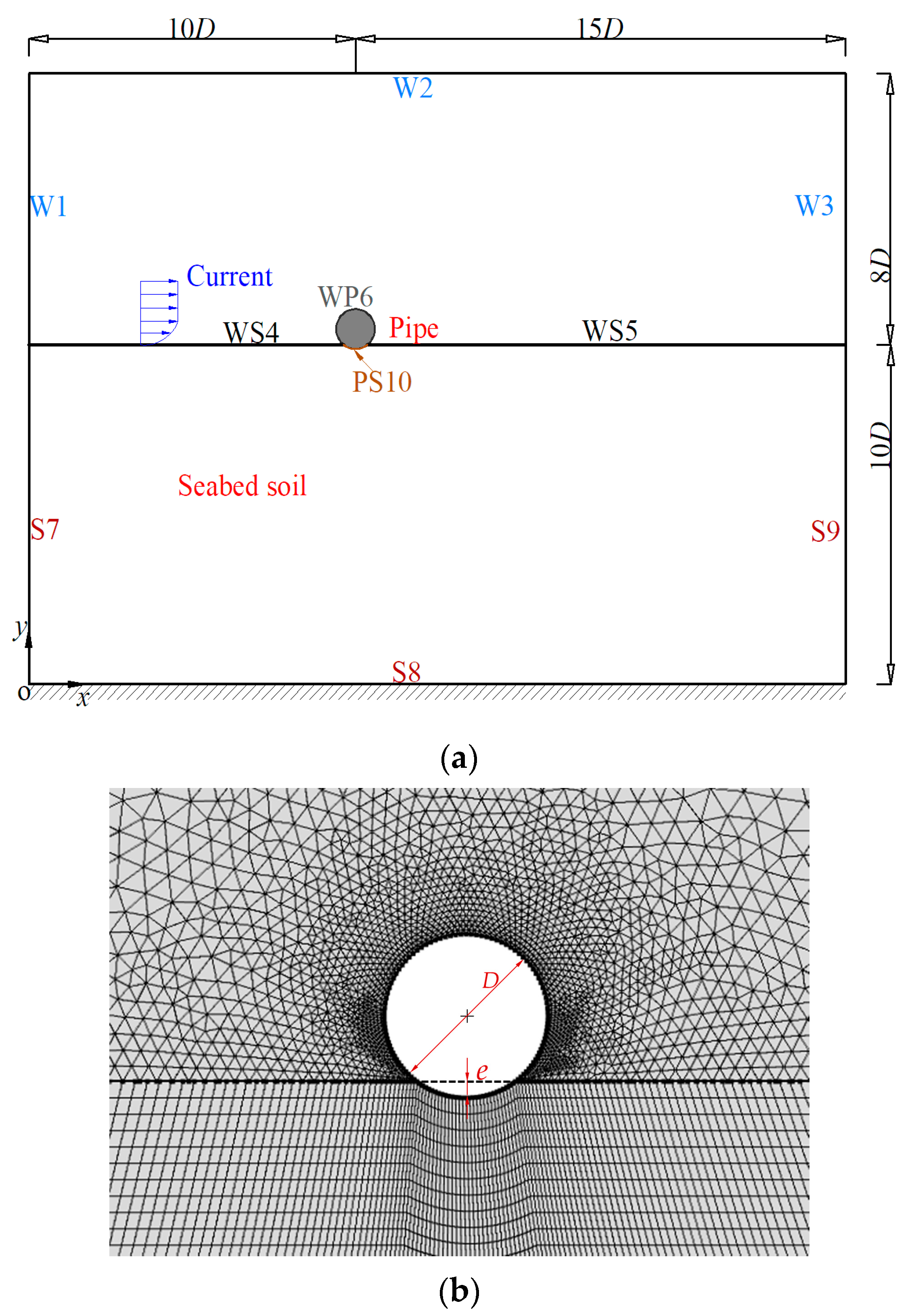
2.2. Geometry and Computational Meshes

As illustrated in Figure 2a, the geometry of the coupled finite element (FE) model mainly consisted of three domains; i.e., the water, the pipeline, and the soil. In the present simulation, a pipe was located on the seabed surface with an embedment (e), the water depth was set as 8D, and the soil depth was chosen as 10D, in which D is the outer diameter of pipe. The left and the right boundaries were 10D and 15D from the center of the pipe, respectively. Such sizes of the water and soil domains were proved to be sufficient to eliminate blockage and boundary effects (see Gao and Luo [20]).

The free triangular meshes were used in the water and the pipe domains, and the structured quadrilateral meshes were generated in the soil domain through a mapped meshing technique. Lagrange elements with order 2 were chosen for the entire domains, and more refined grids were used in proximity to the pipe to ensure the computation accuracy, as shown in Figure 2b. The mesh resolution and mesh element quality were key aspects for the coupled simulation. The mesh quality measures included skewness, maximum angle, volume versus circumradius, etc. The mesh quality could be described with a dimensionless parameter between 0 and 1, where 1 represents a perfectly regular element, and 0 represents a degenerated element [40]. In the present model, the number of all elements was approximately 3 × 10⁴, and the highest resolution was about 0.001 m. A high mesh quality was measured through element statistics (the minimum value of a series of average mesh quality values for different measured aspects was about 0.9), which proved sufficient for guaranteeing the convergence and efficiency of the results.

2.3. Boundary Conditions and Properties of Materials

2.3.1. Boundary Conditions

The boundary conditions were set as follows (see Figure 2a):

• W1 (the inlet of the water domain): a constant undisturbed flow velocity $\overline{u_1}|{}_{x=0}=U$ was specified. The inlet value for the turbulent kinetic energy and dissipation could be evaluated with $k=1.5{\left(U{I}_{\mathrm{t}}\right)}^2$, $\epsilon =C_{\mathsf{\mu }}{}^{3/4}{k}^{3/2}/L_{\mathrm{t}}$, in which turbulent intensity $I_{\mathrm{t}}=0.05$ and turbulence length scale $L_{\mathrm{t}}=0.07\times 8D$ [41].
• W2 (the top of the water domain): a no-flow symmetry boundary was set at y = 18D.
• W3 (the outflow boundary): the pressure was given a reference value p = 0, whereas the other flow variables (velocity, turbulent kinetic energy, dissipation) were allowed to adjust freely with zero x-gradient conditions. The suppressed backflow was selected to prevent fluid from entering the domain through the boundary.
• WS4, WS5 (the water–seabed interface at the left and right of the pipe): the logarithmic wall function [42] was implemented; The effective normal stress and the shear stress vanished: ${\sigma }_{\mathrm{ij}}^{\prime }|{}_{\mathrm{i}\left(\mathrm{j}\right)=1,2}=0$; and the excess pore pressure was equal to the water pressure of the flow field at the surface of the seabed: $u_{\mathrm{w}}|{}_{y=-10D}=p$.
• WP6 (the pipe–water interface): no flow through the impermeable wall of the pipe (i.e., $\partial p/\partial n=0$); similar to WS4 and WS5, the logarithmic wall function was implemented at the pipe–water interface.
• S7, S9 (the left and the right lateral boundaries of the soil domain): no seepage was induced at the lateral boundaries: $\partial u_{\mathrm{w}}/\partial x=0$; and the normal displacement was set as zero: $u^{\mathrm{s}}{}_{\mathrm{i}}|{}_{\mathrm{i}=1}=0$.
• S8 (the bottom of the soil domain): an impermeable fixed bottom was set at y = 0; i.e., zero displacement: $u^{\mathrm{s}}{}_{\mathrm{i}}|{}_{\mathrm{i}=1,2}=0$; and no vertical seepage: $\partial u_{\mathrm{w}}/\partial y=0$.
• PS10 (the pipe–soil interface): the wall of the pipe was assumed to be impermeable, and there was no pore pressure gradient at the pipe surface: $\partial u_{\mathrm{w}}/\partial n=0$. Both the rolling and the sliding motions of the pipe were permitted for the freely laid pipe.
• A contact-pair algorithm was adopted to describe the pipe–soil interfacial behavior [40]. The pipe and seabed surface were assigned as the source and destination boundaries in the contact pair, respectively. Hard contact was chosen for the normal contact, and normal tensile stress was not allowed along the pipe–soil interface. When the pipe–soil contact surface was closed, it conveyed tangential stress. The Coulomb friction theory was used for the interfacial tangent contact. The pipe and the soil in the contact pair adhered to each other if the frictional shear stress (τ) was less than the critical one (τ_crit). Once τ_crit was exceeded, slippage along the interface occurred. In the Coulomb friction model, the friction coefficient (${\mu }_{\mathrm{F}}$) is defined as ${\mu }_{\mathrm{F}}=\tan \left({\phi }_{\mathsf{\mu }}\right)$, where ${\phi }_{\mathsf{\mu }}$ is the friction angle of the pipe–soil interface. The value of ${\phi }_{\mathsf{\mu }}$ generally ranges from 0.5 to 1.0 of the soil friction angle φ, depending on the interface characteristics and relative movement between the pipe and the soil [43]. For a smooth pipe on a sandy seabed, a value of ${\phi }_{\mathsf{\mu }}$ = 0.58$\phi$ was herein considered, thus ${\mu }_{\mathrm{F}}$ = 0.37 was adopted in the present numerical simulations.

2.3.2. Properties of Materials

For the numerical simulations, the properties of the steel pipe, the saturated sandy seabed, and the steady flow are summarized in

Table 1. Properties of the seabed, the current, and the pipe.

Parameters		Values	Units	Notes
Seabed (sand)	Buoyant unit weight of soil (${\gamma }^{\prime }$)	9.3	kN/m3
	Elastic modulus (Es)	30	MPa
	Poisson’s ratio (${\nu }_{\mathrm{s}}$)	0.3
	Angle of internal friction (φ)	35	degree
	Cohesion (c)	0	kPa
	Porosity of soil (n)	0.43
Current (steady flow)	Inflow velocity (U)	0.05~1.50	m/s
	Mass density (${\rho }_{\mathrm{f}}$)	1.0 × 103	kg/m3
	Kinematic viscosity (${\nu }_{\mathrm{f}}$)	1.0 × 10−6	m2/s
Pipe (steel)	Diameter (D)	0.5	m
	Submerged weight per meter (Ws)	1.0	kN/m	Varied in Section 4.3
	Young’s modulus (Ep)	2.1 × 105	MPa
	Poisson’s ratio (${\nu }_{\mathrm{p}}$)	0.2
	Frictional coefficient at the pipe–soil interface (${\mu }_{\mathrm{F}}$)	0.37
	Initial embedment-to-diameter ratio (e/D)	0.10		Varied in Section 4.3

.

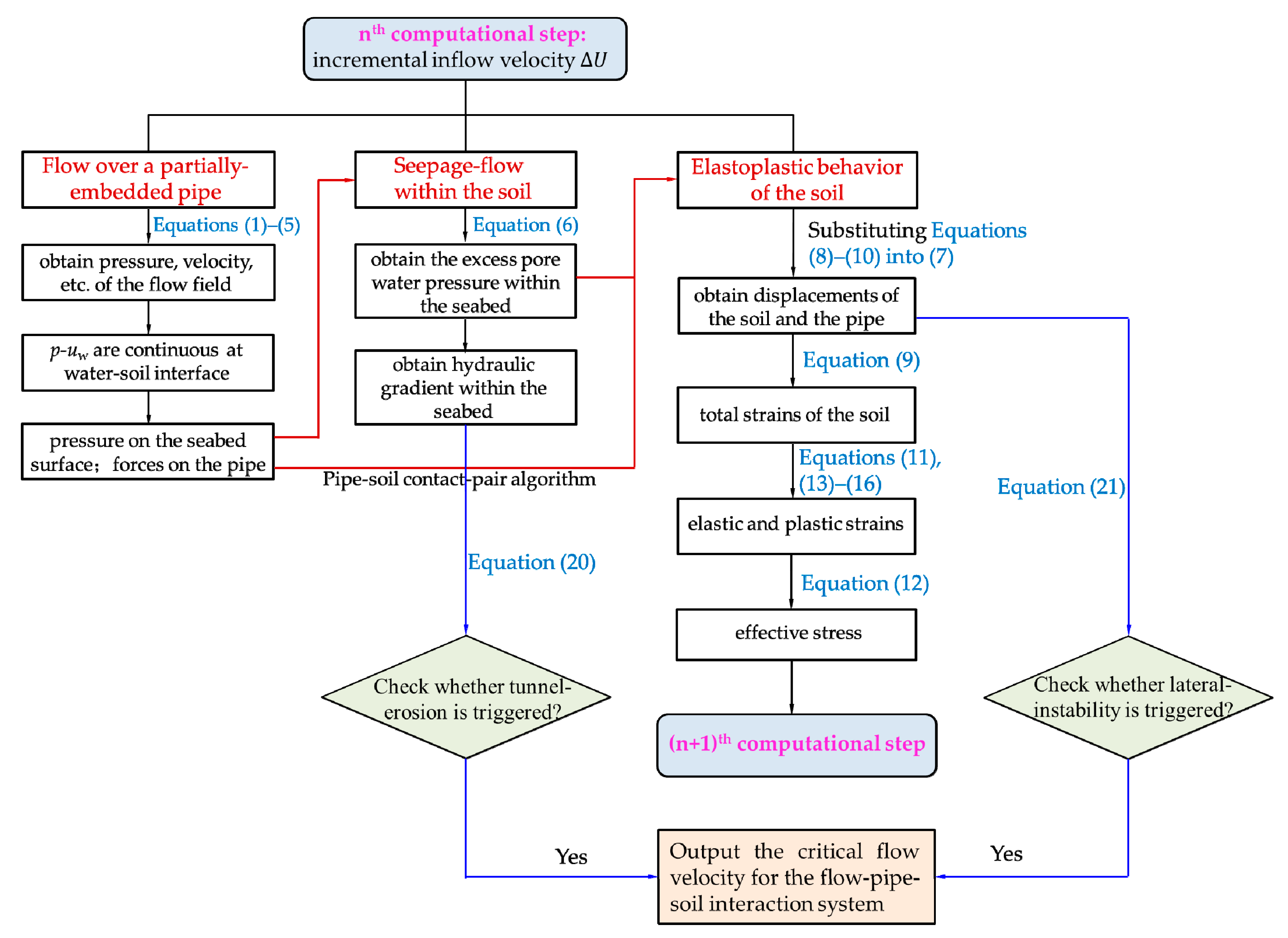
2.4. Coupling Algorithm

The aforementioned governing equations were solved using the software COMSOL Multiphysics with a coupling algorithm to obtain all the variables sequentially, as illustrated in Figure 3.

• Firstly, the responsibility of the flow field over the pipe (Equations (1)–(5)) in one computational step was to determine the pressure around the pipe, and to provide pressure/force acting on the seabed and structures as a surface boundary condition for the geotechnical simulations. As such, the continuity of the water–soil interface pressure (p-u_w) in every computational step was ensured, and the one-way coupling of flow and seepage fields could be implemented.
• Then, by solving the continuity equation (Equation (6)), the pore pressure could be obtained. Substituting the Terzaghi’s effective stress principle (Equation (8)), the relationship between total strain and displacement (Equation (9)), and the elastoplastic constitutive model (Equation (10)) into the stress balance equation (Equation (7)), the governing equation for soil deformation with the unknown variables of soil displacement and pore water pressure could be solved through iterative computation.
• Concurrently, the soil’s total strain, and its elastic and plastic components, could be calculated with the deformation continuity condition (Equation (9)) together with the yield function and the flow rule (Equations (13)–(16)). Based on the constitutive model (Equation (12)), the effective stress within the soil around the partially embedded pipe could be acquired.
• Based on the criteria for the lateral instability and tunnel erosion of the pipe (Equations (20) and (21) in Section 4.2), we could then examine whether the two instability modes were triggered.

3. Verification of Numerical Model

In this section, the proposed numerical model is validated by comparing with the existing experimental or numerical results. Both the pressure distribution at the mudline near the pipe and the critical velocity for the lateral instability of a pipe are examined, respectively.

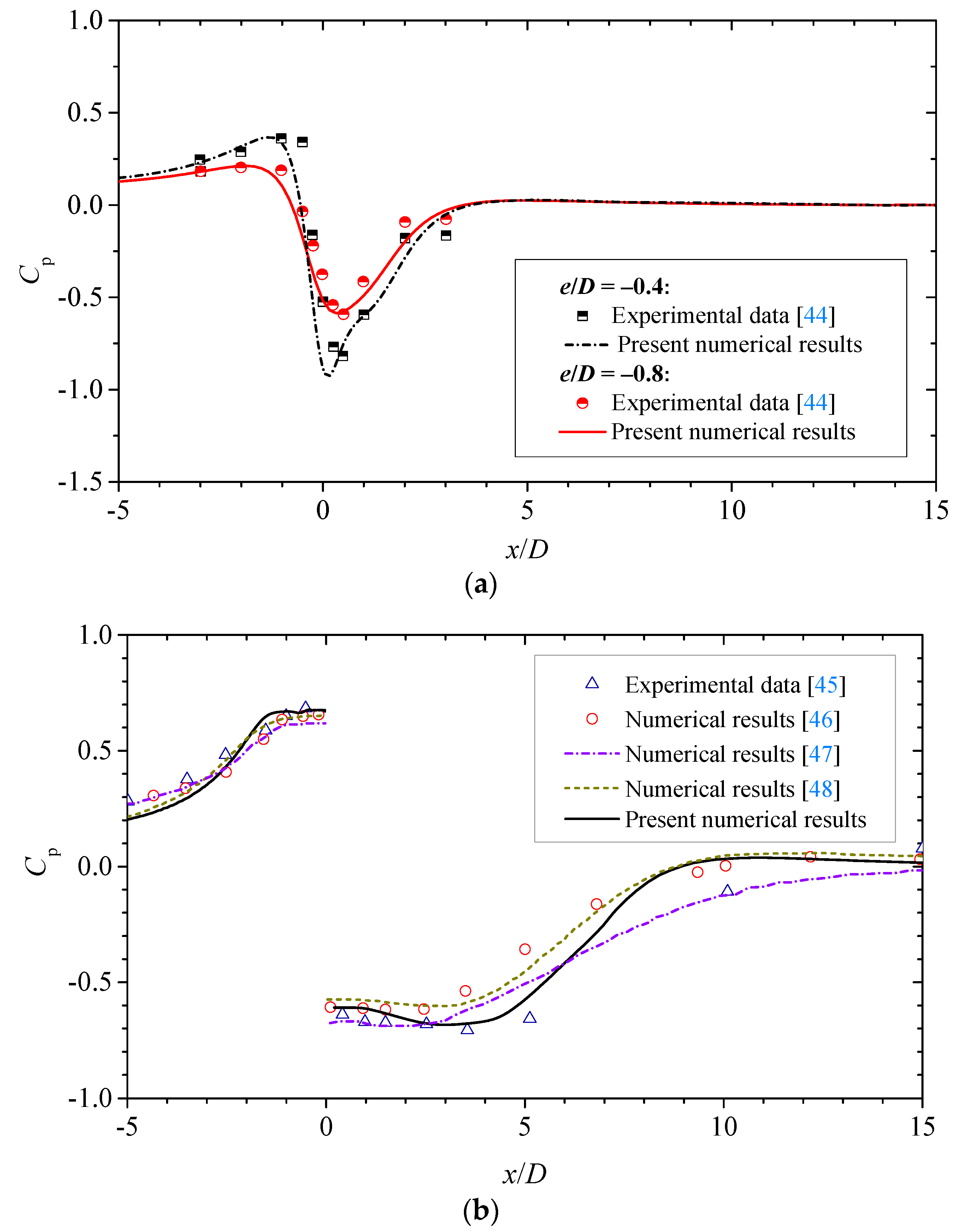
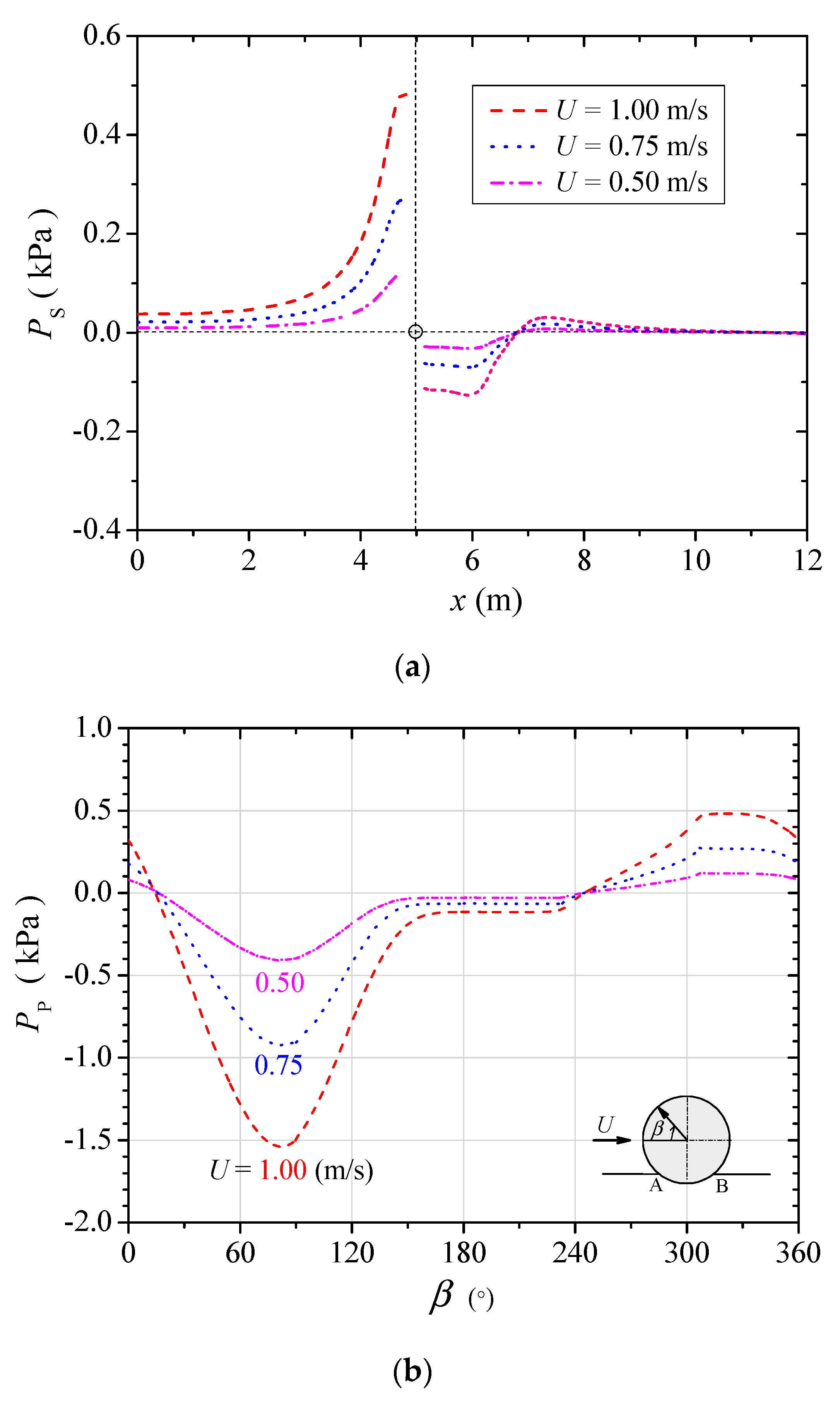
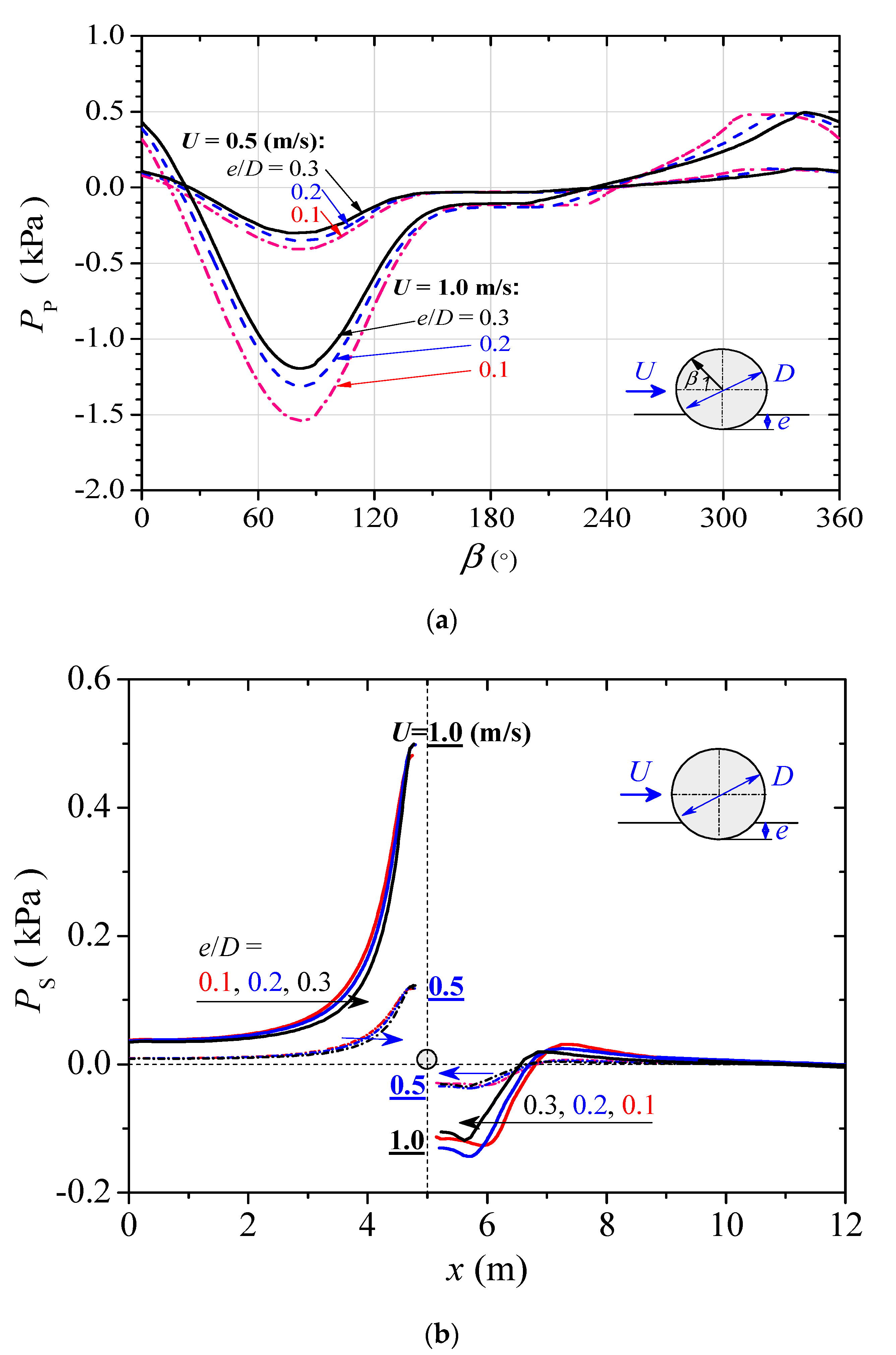
3.1. Pressure Distribution at the Mudline near the Pipe

The proposed model was firstly validated against the existing experimental data regarding pressure distribution at the mudline near the pipe laid above or on the bed surface. The calculated distributions of pressure coefficient (C_p) at the mudline in the proximity of the pipe are plotted in Figure 4a, in which the experimental data of Bearman and Zdravkovich [44] are also provided. The pressure coefficient C_p is defined as follows:

$$C_{\mathrm{p}}=\frac{P_{\mathrm{s}}-P_{\mathrm{r}}}{0.5{\rho }_{\mathrm{f}}{U}^2}$$

(19)

where P_s is the steady-flow-induced pressure at the mudline around the pipe, and $P_{\mathrm{r}}$ is the reference pressure. In the experiments by Bearman and Zdravkovich [44], two values of e/D were examined; i.e., e/D = −0.4, −0.8; and the examined Reynolds number was $Re\left(=UD/{\nu }_{\mathrm{f}}\right)$ = 1.5 × 10⁴. Note that the pipe was located at x/D = 0; the negative value of e/D denoted that the pipe was placed above the bed surface. Similarly, Figure 4b shows the numerical results of the distributions of C_p under the conditions of e/D = 0 (i.e., the pipe was just touching the bed surface) and Re = 4.5 × 10⁴. The experimental measurements by Tsiolakis [45] and the previous numerical results [46,47,48] are also provided in this figure for comparison. As shown in Figure 4, the results of C_p calculated with the present model overall agreed well with the existing experimental and numerical results, indicating that the present model was capable of predicting the flow-induced pressure on the seabed surface in the vicinity of the pipeline.

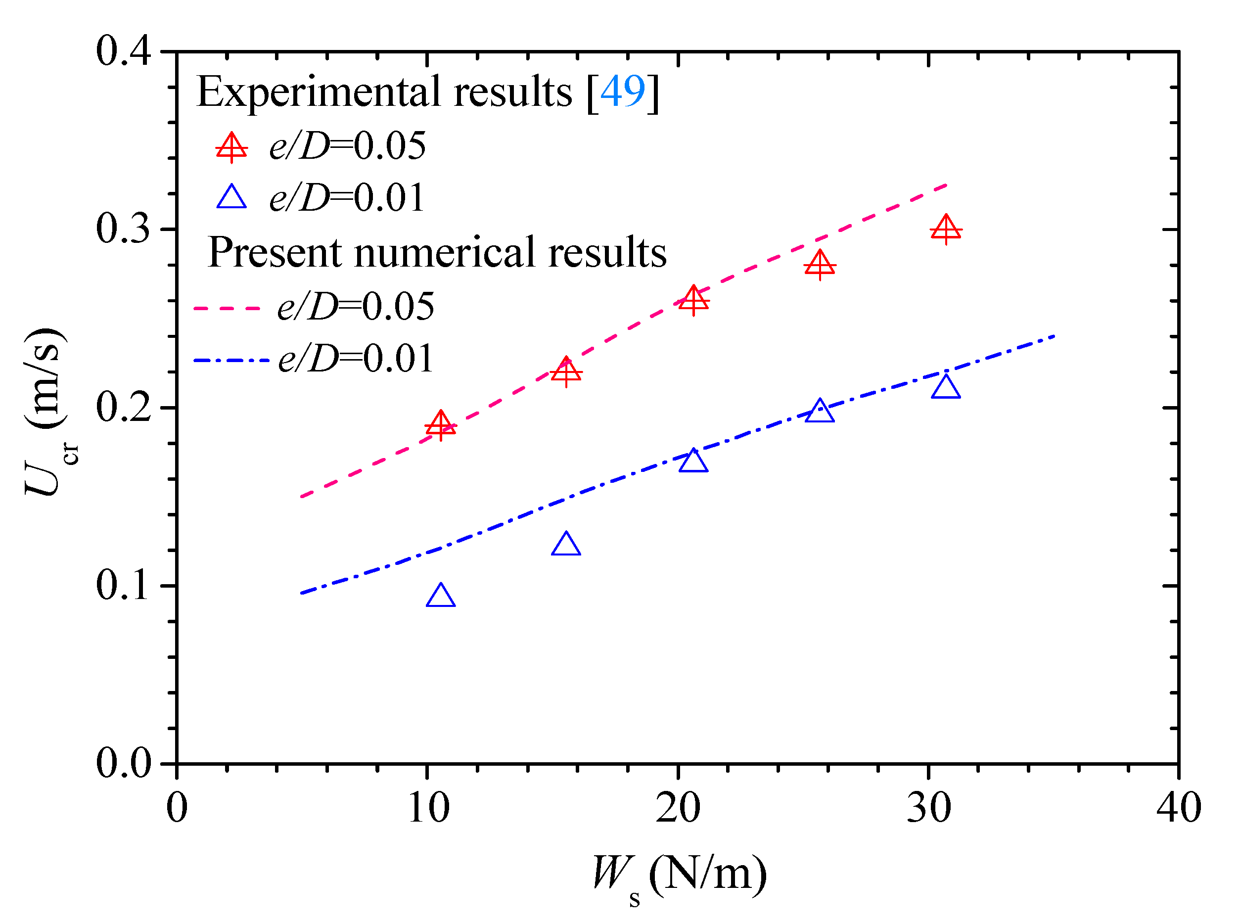
3.2. Critical Velocity for the Lateral Instability of a Pipe

To further verify the proposed numerical model, the steady-current-induced lateral instability of a freely laid pipe was investigated. Recently, a series of tests was conducted in a flow–structure–soil interaction flume (52.0 m long, 1.0 m wide, and 1.5 m high) at the Institute of Mechanics, Chinese Academy of Science (see Xu et al. [49]). A silt bed (5.0 m long, 1.0 m wide, and 0.5 m thick) was prepared in the middle of the flume, and the water depth was kept constant at 0.6 m. The outer diameter of the test pipe D = 0.14 m, and the frictional coefficient at the rough pipe–soil interface ${\mu }_{\mathrm{F}}$ = 0.35 (${\phi }_{\mathsf{\mu }}$ = 0.70$\phi$). The soil properties of the test silts were as follows: d₅₀ = 0.047 mm, ${\gamma }^{\prime }$ = 9.76 kN/m³, n = 0.40, E_s = 20 MPa, ${\nu }_{\mathrm{s}}$ = 0.3, c = 6.3 kPa, $\phi$ = 27.4°.

Figure 5 shows the numerically simulated and the measured critical velocity for the lateral instability (U_cr) with various submerged weights of the pipe (W_s) on the silt bed for two values of e/D; i.e., e/D = 0.01, 0.05. As shown in Figure 5, the present numerical results were in reasonable agreement with the data for flume measurements [49]. The critical flow velocity for pipe instability (U_cr) increased approximately linearly with the submerged weight of the pipe (W_s) for a given value of e/D. For a fixed value of W_s, the critical flow velocity U_cr rose for a larger pipe embedment (e/D). It should be noted that, for the examined fine-grained silts with certain cohesion, tunnel erosion beneath the pipe was not observed in the flume experiments, even for the small embedment; e.g., e/D = 0.01. The proposed coupled FE model was capable of predicting the lateral-instability process by employing the aforementioned contact-pair algorithm for describing the pipe–soil interfacial behavior (see Section 2.3.1).

4. Numerical Results and Discussions

4.1. Flow over and Seepage Flow Beneath a Partially Embedded Pipe

The proposed coupled FE model was employed to explore the competition mechanism between the lateral instability and the tunnel erosion of a freely laid pipeline on a non-cohesive seabed. The input data of all parameters for the sandy seabed, the steady flow, and the pipe are listed in Table 1.

As shown in Figure 6a, for a certain inflow velocity (U = 1.0 m/s), the flow over and the seepage flow beneath the partially embedded pipe could be obtained synchronously, so that the pressure distribution at the water–soil interface was kept continuous. Similar to the observations by Mao [50], due to the presence of the pipe, a large lee-wake vortex was generated at the downstream of pipe, and two small vortices were formed in front and at the rear of the pipe, respectively (see Figure 6b). The flow pressure in front of the pipe was higher than that at the rear of it, which further induced the seepage flow within the soil beneath the pipe. Figure 6b,c give the seepage-flow direction and the contour of hydraulic gradients (i) around the pipe, respectively, indicating the peak values of the hydraulic gradient that emerged at the upstream and downstream corners of the pipe–soil interface (points A and B in Figure 6c). The seepage vectors were generally upward at the downstream zone (see Figure 6b), which could lead to an obliquely upward seepage flow at the seepage exit (i.e., point B in Figure 6c).

Figure 7a,b give the pressure distributions along the mudline (P_S) and around the pipe surface (P_P) for various inflow velocities (U), respectively. It is indicated that the flow-induced pressure was generally positive at the upstream of the partially embedded pipe, while negative at the downstream. As the flow velocity increased, the pressure drop increased gradually. The hydrodynamic forces on the partially embedded smooth pipe could be calculated by integrating the pressure distribution around the pipe surface in the water domain (see Figure 2a), which could be decomposed into the in-line (drag force F_D) and cross-flow (lift force F_L) components. Figure 8 gives the variations of drag force on the pipe (F_D) and the hydraulic gradient at the seepage exit (i_ex) within the soil. As shown in Figure 8, the values of both F_D and i_ex increased nonlinearly with the increase of flow velocity (U), which played decisive roles for triggering either the lateral instability or the tunnel erosion of the pipe.

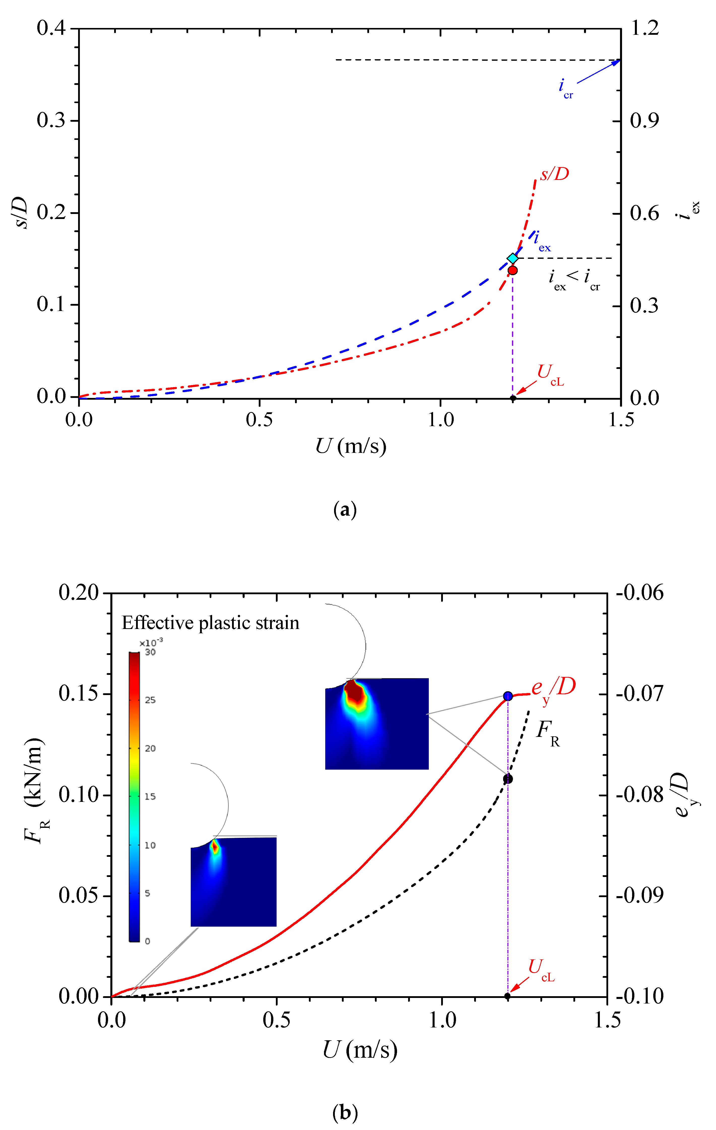
4.2. Competition between Tunnel Erosion and Lateral Instability

As stated above, the seepage failure beneath the pipe resulting from a pressure drop was recognized as the dominant cause of the onset of tunnel erosion. To quantitatively predict the onset of tunnel erosion under the action of a steady current, the critical hydraulic gradient for the vertical seepage failure, $i_{\mathrm{cr}0}=\left(1-n\right)\left(G_{\mathrm{s}}-1\right)$, was adopted in previous analyses (e.g., Sumer et al. [18]; Zang et al. [47]; Zhang et al. [21]). Note that G_s is the specific gravity of soil grains. As indicated in Figure 6b, the direction of seepage flow at the exit (point B) was tangent to the pipe surface instead of upward vertically. As such, in the present study, the criterion for the oblique seepage failure proposed by Gao and Luo [20] was employed; i.e., the hydraulic gradient at the seepage exit (i_ex) was beyond the critical value (i_cr):

$$i_{\mathrm{ex}}>i_{\mathrm{cr}}=\left(\sin \theta +\cos \theta \hspace{0.17em}\tan \phi \right)i_{\mathrm{cr}0}$$

(20)

where $\theta$ is the embedment angle of the pipe (see Figure 8).

With increasing flow velocity of ocean currents, if the lateral soil resistance (F_R) was insufficient to balance the drag force (F_D), i.e., F_D > F_R, the pipe would break out from its original location. As observed in the flume experiments (also see Gao et al. [14]), the pipe breakout (or the lateral instability) generally occurred suddenly with a relatively large lateral displacement. In the present numerical simulations, the criterion for the lateral instability of the pipe was adopted as follows:

$$U>U_{\mathrm{cL}} \mathrm{while} \left({s|}_{U=U_{\mathrm{cL}}+\Delta U}-{s|}_{U=U_{\mathrm{cL}}}\right)/\left({s|}_{U=U_{\mathrm{cL}}}-{s|}_{U=U_{\mathrm{cL}}-\Delta U}\right)>\delta$$

(21)

where U_cL is the critical flow velocity for the lateral instability of the pipe, s is the lateral displacement of the pipe at an increasing flow velocity (U) with a velocity increment $\Delta U$ (=0.05 m/s), and $\delta$ is a judging constant (choosing $\delta =2.0$).

Figure 9a shows the lateral displacement of the pipe (s/D) and the maximum upward hydraulic gradient (i_ex) with the increase of flow velocity (U), respectively. It is indicated that the values of s/D increased gradually with the increase of U until its critical value was reached (e.g., U_cL = 1.20 m/s). The embedded pipe moved obliquely upward progressively (see Figure 9b). As shown in Figure 9b, at a relatively lower flow velocity, the plastic-strain zone was generated dominantly beneath the pipe, especially at the pipe–mudline corners; with further increasing U, the plastic strains extended successively and the soil resistance (F_R) was increased correspondingly, resulting in a squeezed plastic zone at the rear of the pipe. According to the criterion (Equation (21)), the critical flow velocity (U_cL) for lateral instability could be obtained. It should be noted that, in the process of such lateral instability, the seepage flow was generated concurrently within the soil (see Figure 6), although i_ex was lower than its critical value for tunnel erosion (i.e.,$i_{\mathrm{ex}}<i_{\mathrm{cr}}$ (=1.10); see Figure 9a) in this case study. That is, under the action of ocean currents, the competition between the tunnel erosion and the lateral instability always existed for a pipeline partially embedded in a non-cohesive seabed.

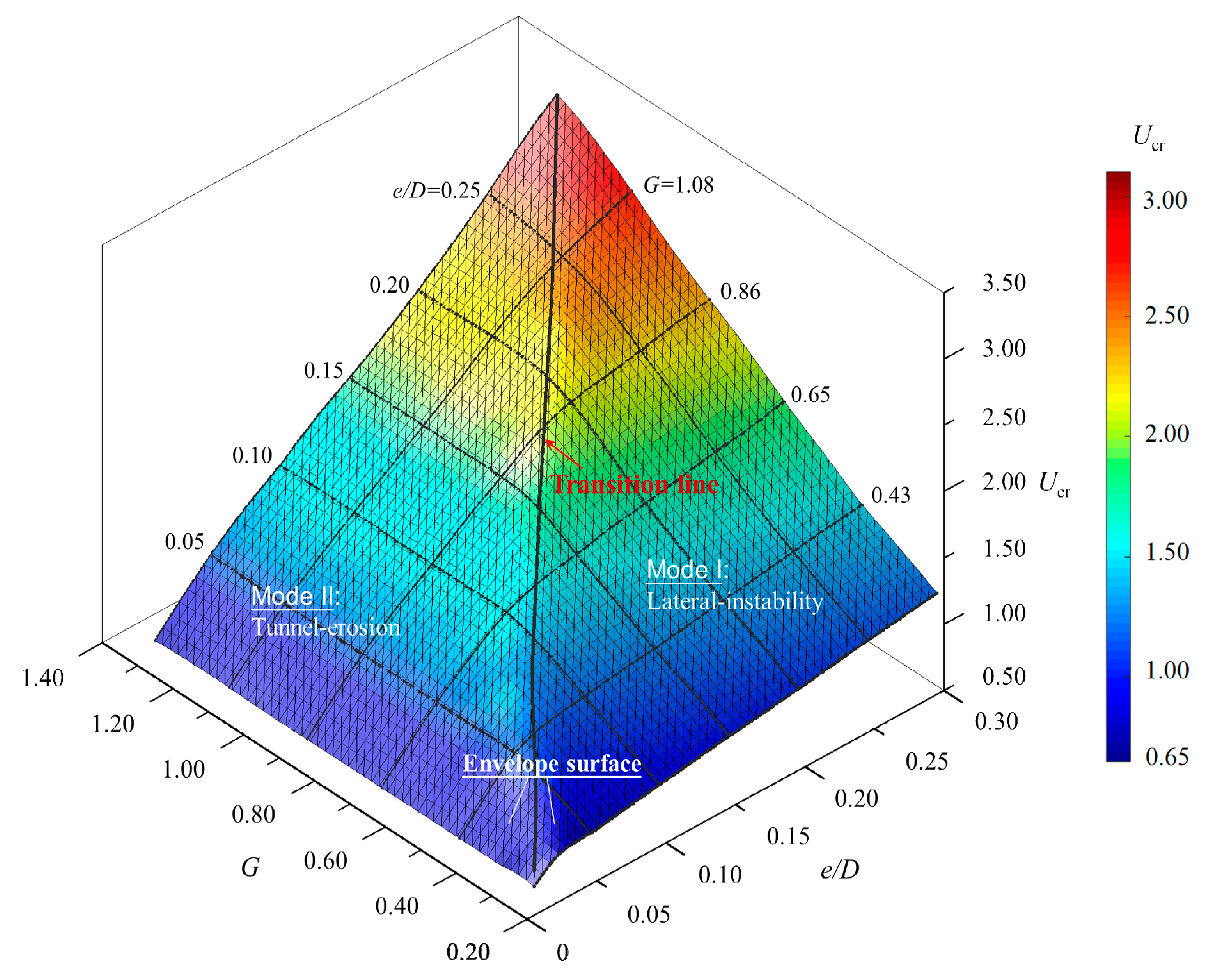
4.3. Instability Envelope: Effects of the Initial Embedment and the Submerged Weight of the Pipe

As aforementioned, if the basic properties of the seabed and the pipeline are given, the critical flow velocity for the pipeline instability (U_cr) will be mainly related to the two dimensionless parameters; i.e., the embedment-to-diameter ratio (e/D) and the non-dimensional submerged weight of the pipeline (G = $W_{\mathrm{s}}/\left({\gamma }^{\prime }{D}^2\right)$ (see Shi and Gao [23]). The proposed coupled FE model was employed to examine the effects of e/D and G on U_cr.

Figure 10a,b show the distributions of the pressure along the pipe surface (P_P) and along the mudline near the pipe (P_s), respectively, for various values of e/D and the flow velocity U. As shown in Figure 10, the flow-induced pressure distributed non-uniformly along the pipe surface and along the mudline. For a fixed value of U (=0.5, or 1.0 m/s), the values of P_P increased gradually with increasing e/D from 0.1 to 0.3, especially at the top of the pipe ($0<\beta <{180}^{°}$; see Figure 10a); accordingly, the values of P_s increased slightly (see Figure 10b).

Figure 11a,b show the variations of the drag force on the pipe (F_D) and those of the hydraulic gradient at the seepage exit (i_ex) with the increase of flow velocity (U), respectively, for various values of e/D. It is indicated that both F_D and i_ex increased nonlinearly with increasing U. For a fixed value of U, the values of both F_D and i_ex decreased with increasing e/D, which could be attributed to the variations of pressure distributions of P_P and P_s with e/D (see Figure 10). Such a reduction in the drag force on the pipe due to increasing embedment was suggested in the existing Det Norske Veritas recommended practice [10]. It seems that the pipe embedment (e/D) had a slight effect on the pressure drop (P_s) along the mudline (see Figure 10b), but its effect on the hydraulic gradient at the exit (i_ex) became much more significant due to the enlargement of the seepage path with a slight increase of e/D (e.g., from 0.1 to 0.3; see Figure 11b).

The submerged weight of the pipe (W_s) may induce plastic strains within the soil beneath the pipe (see Figure 9), and further, has influence on the lateral resistance (F_R) to the partially embedded pipe under the action of ocean currents. Figure 12 shows the variations of F_R with the flow velocity (U) for various values of the non-dimensional submerged weight of the pipe (G). As indicated in Figure 12, for a fixed value of G, the higher values of F_R could be mobilized to balance the drag force (F_D) in a flow with increasing U. A heavier pipe with larger G would become more stable; i.e., a larger value of F_R was mobilized to resist a higher inflow velocity U.

To quantitatively characterize the competition mechanism between lateral instability and tunnel erosion, a series of simulations was conducted with the proposed model. In the following parametric study, the values of e/D and G were varied, and the values of other parameters are given in Table 1. As aforementioned, following the calculation procedure for the coupled flow-seepage-elastoplastic model (see Figure 3), the critical flow velocity (U_cr) for the lateral instability or the tunnel erosion could be obtained. The effects of the embedment-to-diameter ratio (e/D) and non-dimensional submerged weight of the pipe (G) on the critical flow velocity (U_cr) were further examined numerically.

Figure 13a,b show the variations of U_cr with e/D for various values of G, and the variations of U_cr with G for various values of e/D, respectively. It is indicated in Figure 13a that, for a given value of G, there existed a transition point from the “tunnel-erosion” (T-mode) to the “lateral-instability” (L-mode) on the critical instability line; the tunnel erosion was more prone to being triggered than the lateral instability for smaller values of e/D. With the increase of G, the values of U_cr and the corresponding e/D for the transition points were both increased concurrently. For a heavy pipe; e.g., G = 1.29, only the T-mode was triggered (that is, the L-mode was suppressed) for the examined range of e/D (0.01 < e/D < 0.30; see the blue line in Figure 13a). Similarly, as shown in Figure 13b, for a pipe with a relatively larger embedment; e.g., e/D = 0.25, the L-mode was much easier to trigger in the examined range of G (0.22 < G < 1.29).

The instability envelope for the flow–pipe–soil interaction could be further established, as shown in Figure 14, and could be described by three controlling parameters; i.e., U_cr, e/D, and G. As illustrated in this figure, the entire instability envelope was a smoothly curved surface and had two components; i.e., Model-I: Lateral-instability (L-mode), and Model-II: Tunnel-erosion (T-mode); while in between T-mode and L-mode was a transition line. If the flow velocity of ocean currents went beyond the instability envelope, either the T-mode or L-mode of the pipe instability could be induced. It was implied that, for a lighter (smaller G) and more deeply embedded (larger e/D) pipe, lateral instability (L-mode) would be more prone to occur; otherwise, tunnel erosion (T-mode) would be more prone to occur.

5. Conclusions

Under the action of ocean currents, two typical instability modes could be triggered; i.e., the lateral instability of the pipe and the tunnel erosion of the underlying soil, which involve complex fluid–pipe–soil interactions. Nevertheless, these two instability modes were only investigated separately in the past. In this paper, the competition mechanism between lateral instability and tunnel erosion of a freely laid pipeline on a non-cohesive seabed was investigated numerically. The following conclusions could be drawn:

• A coupled flow-seepage-elastoplastic modeling approach was proposed that could realize the synchronous simulation of the pipe hydrodynamics, the seepage flow, and the elastoplastic behavior of the soil beneath the pipe. The proposed model was verified through experimental and numerical results.
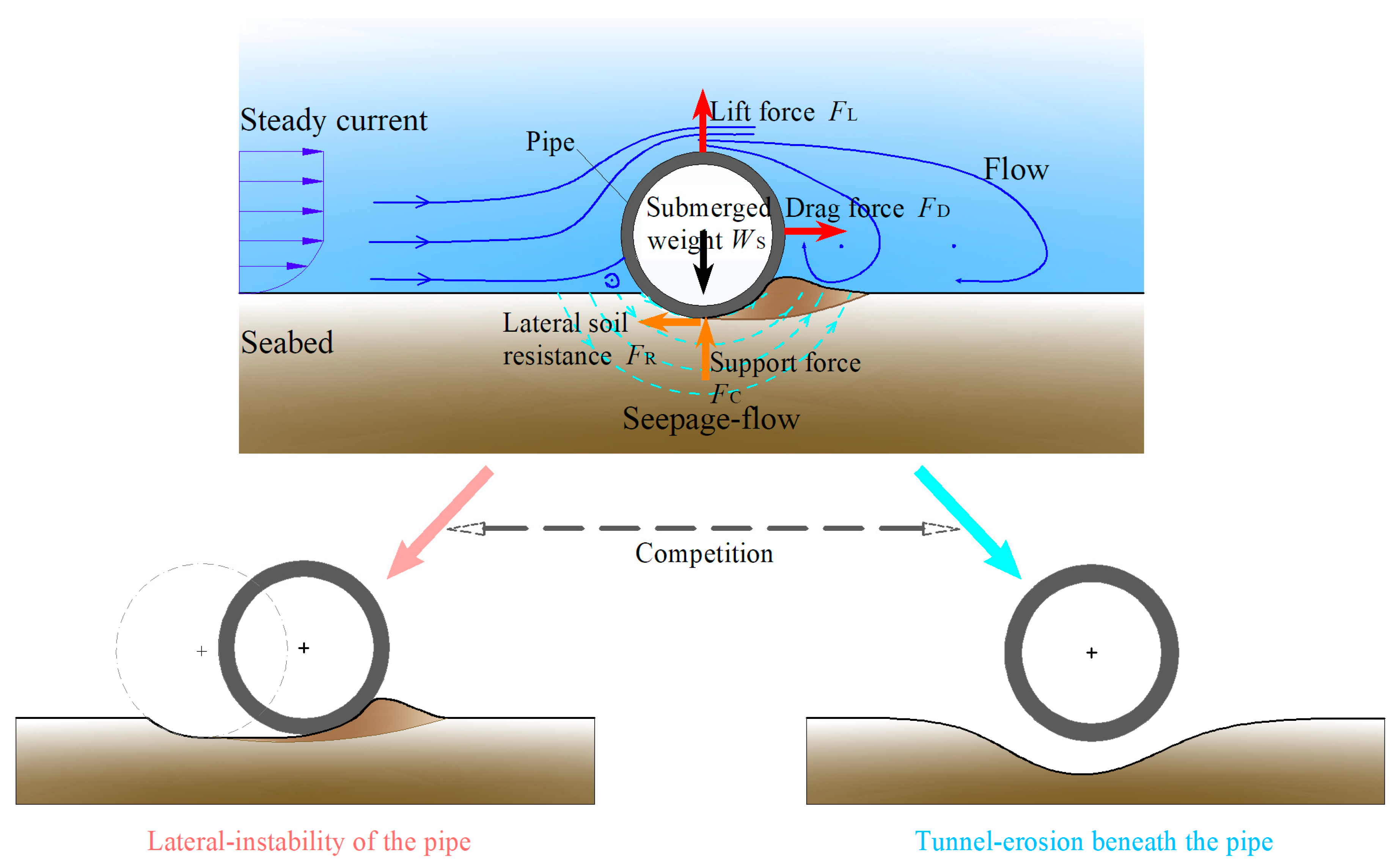
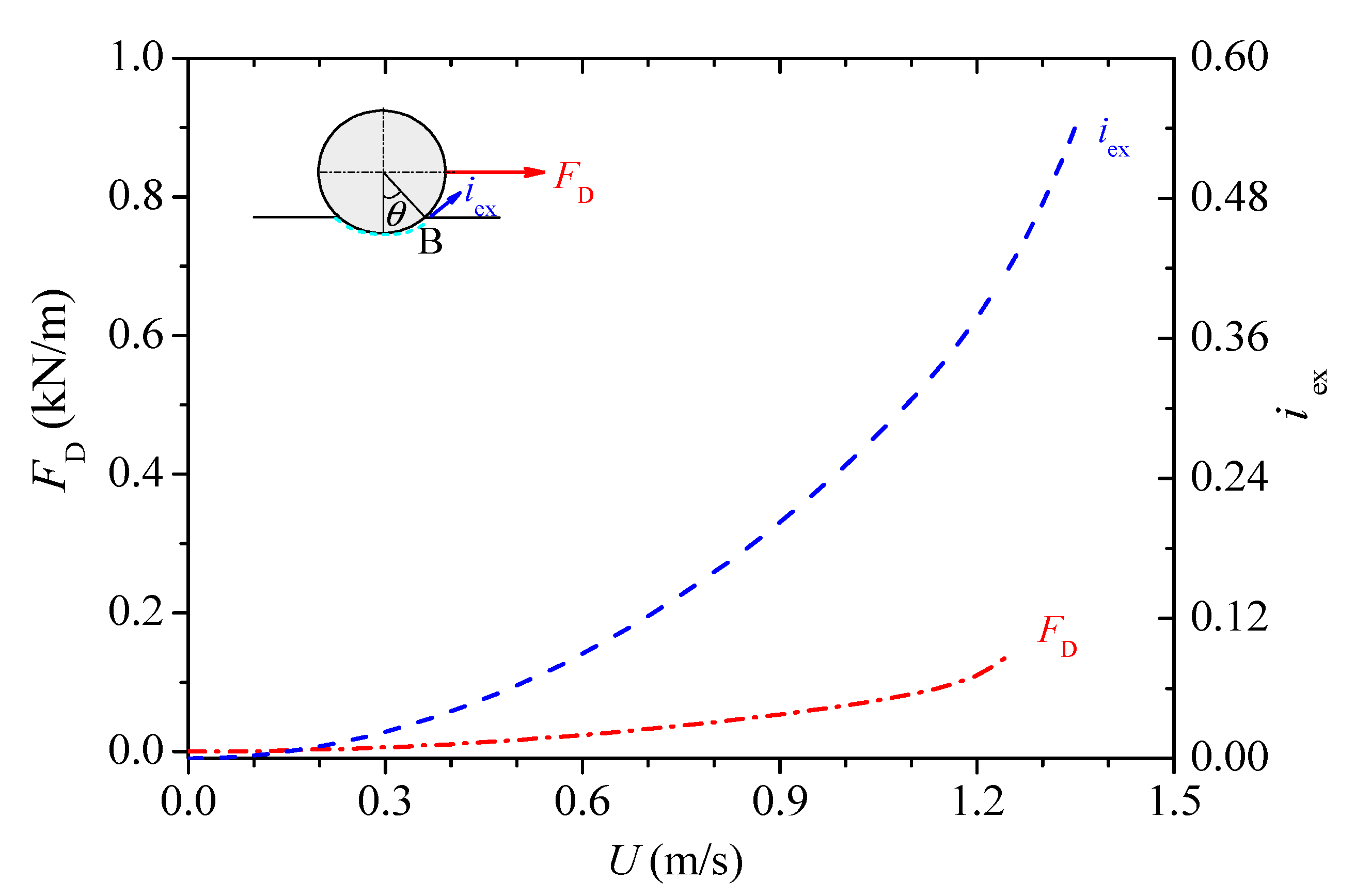
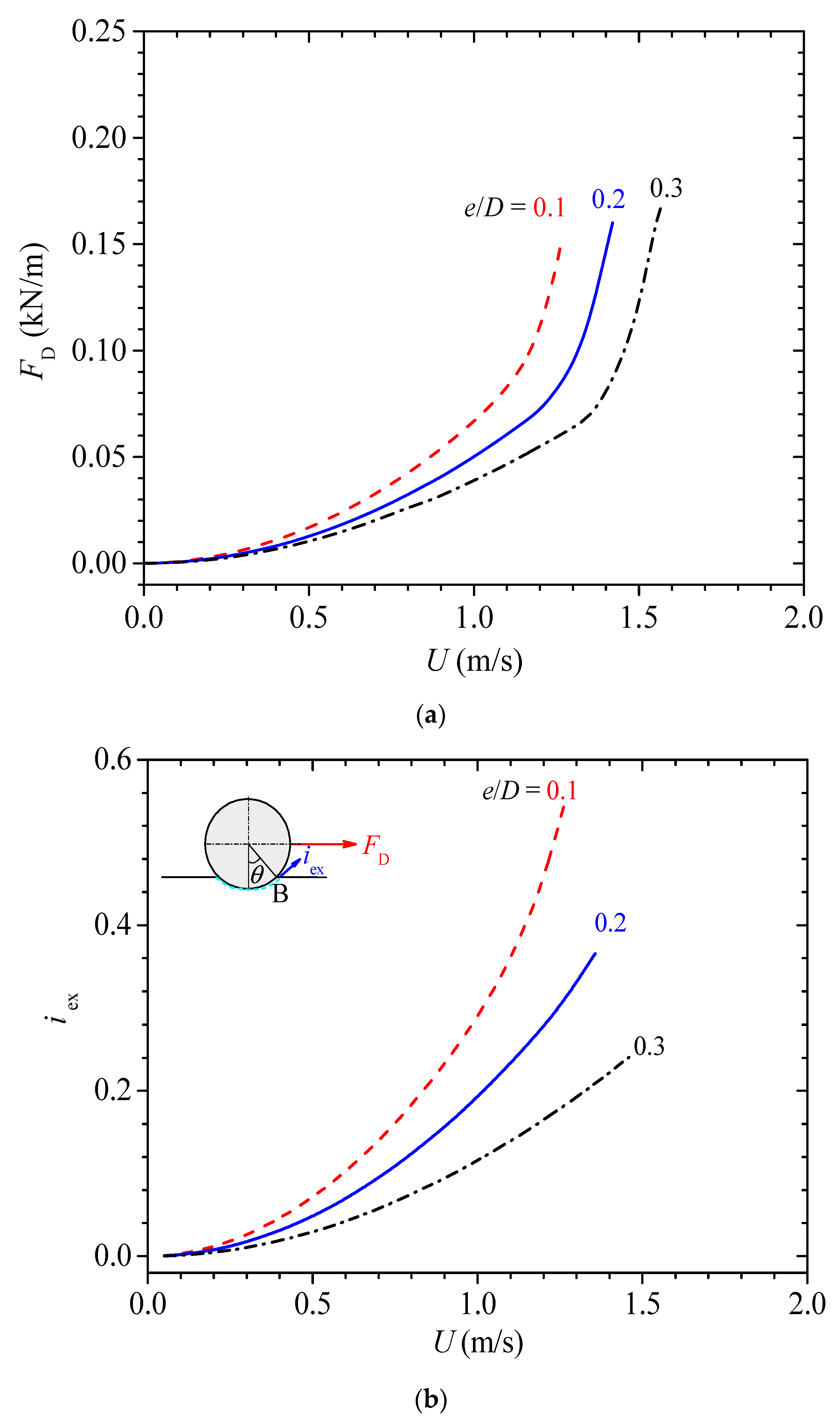
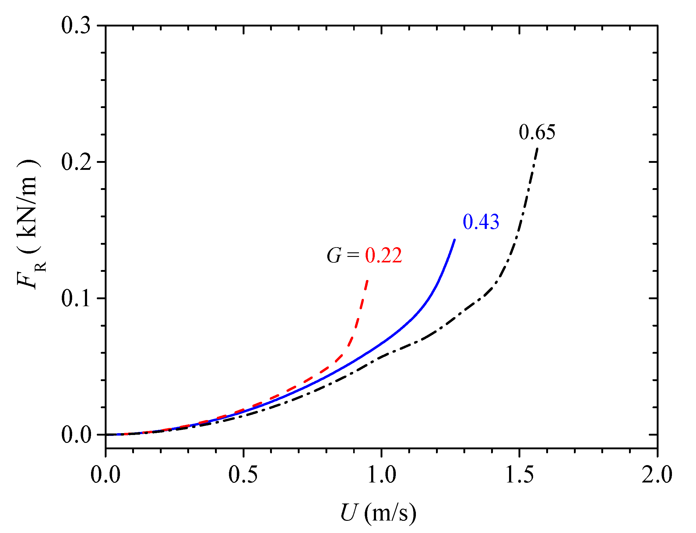
• Both the drag force on the pipe and the hydraulic gradient at the seepage exit beneath the pipe increased concurrently with increasing flow velocity, which could induce either the lateral instability of pipe or the tunnel erosion of soil. The competition between such two instability modes always existed for a partially embedded pipe.
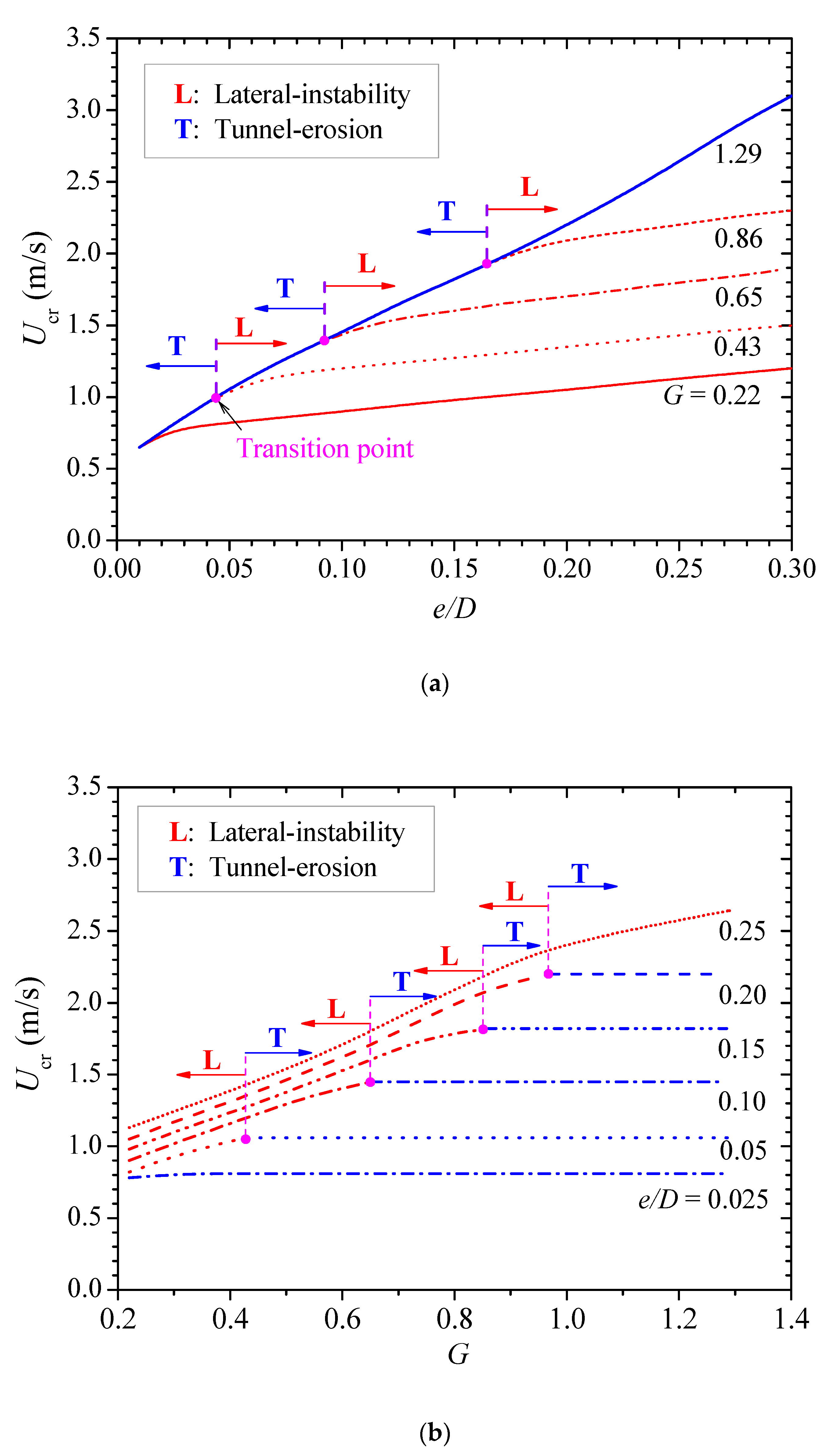
• A parametric study indicated that there generally existed a transition point from tunnel erosion to lateral instability on the critical instability line representing the variation of critical flow velocity (U_cr) with embedment-to-diameter ratio (e/D) for various values of a non-dimensional submerged weight of the pipe (G), or the variation of U_cr with G for various values of e/D. Tunnel erosion was more prone to being triggered than lateral instability for smaller values of the embedment-to-diameter ratio.
• The instability envelope for the flow–pipe–soil interaction system was eventually established, and could be described by three parameters; i.e., U_cr, e/D, and G. It was implied that, for a lighter (smaller G) and more deeply embedded (larger e/D) pipe, lateral instability would be more prone to occur; otherwise, tunnel erosion would be more prone to take place.

References

1. Zhang, G.C.; Qu, H.; Chen, G.J.; Zhao, C.; Zhang, F.L.; Yang, H.Z.; Zhao, Z.; Ma, M. Giant discoveries of oil and gas fields in global deepwaters in the past 40 years and the prospect of exploration. J. Nat. Gas Sci. 2019, 4, 1–28. [Google Scholar] [CrossRef]
2. Wang, H.H.; Liu, G.H. Statistics and analysis of subsea pipeline accidents of CNOOC. China Offshore Oil Gas 2017, 29, 157–160. [Google Scholar]
3. Fredsøe, J. Pipeline–seabed interaction. J. Water. Port Coast. 2016, 142, 1–20. [Google Scholar] [CrossRef] [Green Version]
4. Gao, F.P. Flow-pipe-soil coupling mechanisms and predictions for submarine pipeline instability. J. Hydrodyn. 2017, 29, 763–773. [Google Scholar] [CrossRef]
5. Drumond, G.P.; Pasqualino, I.P.; Pinheiro, B.C.; Estefen, S.F. Pipelines, risers and umbilicals failures: A literature review. Ocean Eng. 2018, 148, 412–425. [Google Scholar] [CrossRef]
6. Shanmugam, G. Contourites: Physical oceanography, process sedimentology, and petroleum geology. Petrol. Explor. Dev. 2017, 44, 183–216. [Google Scholar] [CrossRef]
7. Gao, F.P.; Gu, X.Y.; Jeng, D.S.; Teo, H.T. An experimental study for wave-induced instability of pipelines: The breakout of pipelines. Appl. Ocean Res. 2002, 24, 83–90. [Google Scholar] [CrossRef]
8. Gao, F.P.; Gu, X.Y.; Jeng, D.S. Physical modeling of untrenched submarine pipeline instability. Ocean Eng. 2003, 30, 1283–1304. [Google Scholar] [CrossRef]
9. Wagner, D.A.; Murff, J.D.; Brennodden, H.; Sveggen, O. Pipe-soil interaction model. J. Water. Port Coast. 1989, 115, 205–220. [Google Scholar] [CrossRef]
10. Det Norske Veritas (DNV). On-Bottom Stability Design of Submarine Pipeline; DNV Recommended Practice DNV-RP-F109; Det Norske Veritas: Oslo, Norway, 2010. [Google Scholar]
11. Det Norske Veritas and Germanischer Lloyd (DNVGL). Free Spanning Pipelines; DNV Recommended Practice DNV-RP-F105; Det Norske Veritas and Germanischer Lloyd: Oslo, Norway, 2017. [Google Scholar]
12. Verley, R.L.P.; Sotberg, T. A soil resistance model for pipeline placed on sandy soils. J. Offshore Mech. Arct. Eng. 1994, 116, 145–153. [Google Scholar] [CrossRef]
13. Verley, R.L.P.; Lund, K.M. A soil resistance model for pipelines placed on clay soils. In Proceedings of the 14th International Conference on Offshore, Marine and Arctic Engineering, Copenhagen, Demark, 18–22 June 1995; pp. 225–232. [Google Scholar]
14. Gao, F.P.; Yan, S.M.; Yang, B.; Wu, Y.X. Ocean currents-induced pipeline lateral stability on sandy seabed. J. Eng. Mech. 2007, 133, 1086–1092. [Google Scholar] [CrossRef] [Green Version]
15. An, H.W.; Luo, C.C.; Cheng, L.; White, D. A new facility for studying ocean-structure-seabed interactions: The O-tube. Coast. Eng. 2013, 82, 88–101. [Google Scholar] [CrossRef]
16. Griffiths, T.; Draper, S.; White, D.; Cheng, L.; An, H.W.; Fogliani, A. Improved stability design of subsea pipelines on mobile seabeds: Learnings from the STABLEpipe JIP. In Proceedings of the 37th International Conference on Ocean, Offshore and Arctic Engineering, Madrid, Spain, 17–22 June 2018. [Google Scholar]
17. Chiew, Y.M. Mechanics of local around submarine pipeline. J. Hydraul. Eng. 1990, 4, 515–529. [Google Scholar] [CrossRef]
18. Sumer, B.M.; Truelsen, C.; Sichmann, T.; Fredsøe, J. Onset of scour below pipelines and self-burial. Coast. Eng. 2001, 42, 313–335. [Google Scholar] [CrossRef]
19. Gao, F.P.; Yang, B.; Yan, S.M.; Wu, Y.X. Occurrence of spanning of a submarine pipeline with initial embedment. In Proceedings of the 6th International Offshore and Polar Engineering Conference, Lisbon, Portugal, 1–6 July 2007; pp. 887–891. [Google Scholar]
20. Gao, F.P.; Luo, C.C. Flow-pipe-seepage coupling analysis of spanning initiation of a partially-embedded pipeline. J. Hydrodyn. 2010, 22, 478–487. [Google Scholar] [CrossRef] [Green Version]
21. Zhang, Q.; Draper, S.; Cheng, L.; An, H.W. Effect of limited sediment supply on sedimentation and the onset of tunnel scour below subsea pipelines. Coast. Eng. 2016, 116, 103–117. [Google Scholar] [CrossRef]
22. White, D.J.; Clukey, E.C.; Randolph, M.F.; Boylan, N.P.; Bransby, M.F.; Zakeri, A.; Hill, A.J.; Jaeck, C. The state of knowledge of pipe-soil interaction for on-bottom pipeline design. In Proceedings of the Annual Offshore Pipeline Technology Conference, Houston, TX, USA, 17–22 June 2017. [Google Scholar]
23. Shi, Y.M.; Gao, F.P. Lateral instability and tunnel erosion of a submarine pipeline: Competition mechanism. Bull. Eng. Geol. Environ. 2018, 77, 1069–1080. [Google Scholar] [CrossRef] [Green Version]
24. Gao, F.P.; Wang, N.; Li, J.H.; Han, X.T. Pipe-soil interaction model for current-induced pipeline instability on a sloping sandy seabed. Can. Geotech. J. 2016, 53, 1822–1830. [Google Scholar] [CrossRef] [Green Version]
25. Qi, W.G.; Shi, Y.M.; Gao, F.P. Uplift soil resistance to a shallowly-buried pipeline in the sandy seabed under waves: Poro-elastoplastic modeling. App. Ocean. Res. 2020, 95, 102024. [Google Scholar] [CrossRef]
26. Gao, F.P.; Wu, Y.X. Non-linear wave induced transient response of soil around a trenched pipeline. Ocean Eng. 2006, 33, 311–330. [Google Scholar] [CrossRef] [Green Version]
27. Shih, T.H. Some developments in computational modeling of turbulent flows. Fluid Dyn. Res. 1997, 20, 67–96. [Google Scholar] [CrossRef]
28. Durbin, P.A. Some recent developments in turbulence closure modeling. Annu. Rev. Fluid Mech. 2018, 50, 77–103. [Google Scholar] [CrossRef]
29. Liang, D.F.; Cheng, L. Numerical modeling of flow and scour below a pipeline in currents Part I. Flow simulation. Coast. Eng. 2005, 52, 25–42. [Google Scholar] [CrossRef]
30. Launder, B.E.; Spalding, D.B. The numerical computation of turbulent flow. Comput. Methods Appl. Mech. Eng. 1974, 3, 269–289. [Google Scholar] [CrossRef]
31. Rodi, W. Turbulence Models and Their Application in Hydraulics: A State of the Art Review, 3rd ed.; Balkema: Rotterdam, The Netherlands, 1993. [Google Scholar]
32. Biot, M.A. General theory of three-dimensional consolidation. J. Appl. Phys. 1941, 12, 155–164. [Google Scholar] [CrossRef]
33. Potts, D.M.; Zdravkovic, L. Finite Element Analysis in Geotechnical Engineering: Theory; Thomas Telford: London, UK, 2001. [Google Scholar]
34. Chang, C.S.; Yin, Z.Y. Micromechanical modeling for behavior of silty sand with influence of fine content. Int. J. Solids Struct. 2011, 48, 2655–2667. [Google Scholar] [CrossRef] [Green Version]
35. Jin, Y.F.; Yin, Z.Y.; Shen, S.L.; Zhang, D.M. A new hybrid real-coded genetic algorithm and its application to parameters identification of soils. Inverse Probl. Sci. Eng. 2017, 25, 1343–1366. [Google Scholar] [CrossRef]
36. Yin, Z.Y.; Wu, Z.Y.; Hicher, P.Y. Modeling the monotonic and cyclic behavior of granular materials by an exponential constitutive function. J. Eng. Mech. 2018, 144, 04018014. [Google Scholar] [CrossRef]
37. Jin, Y.F.; Yin, Z.Y.; Wu, Z.X.; Daouadji, A. Numerical modeling of pile penetration in silica sands considering the effect of grain breakage. Finite Elem. Anal. Des. 2018, 144, 15–29. [Google Scholar] [CrossRef] [Green Version]
38. Drucker, D.C.; Prager, W. Soil mechanics and plastic analysis on limit design. J. Appl. Math. 1952, 10, 157–165. [Google Scholar] [CrossRef] [Green Version]
39. Jin, Z.; Yin, Z.Y.; Kotronis, P.; Li, Z. Advanced numerical modelling of caisson foundations in sand to investigate the failure envelope in the H-M-V space. Ocean Eng. 2019, 190, 106394. [Google Scholar] [CrossRef] [Green Version]
40. COMSOL Multiphysics. COMSOL Multiphysics® Reference Guide Version 5.3a; COMSOL AB: Stockholm, Sweden, 2017. [Google Scholar]
41. Versteeg, H.K.; Malalasekera, W. An Introduction to Computational Fluid Dynamics-The Finite Volume Method; Pearson Prentice Hall: London, UK, 1995. [Google Scholar]
42. Launder, B.E. Numerical computation of convective heat transfer in complex turbulent flows: Time to abandon wall functions. Int. J. Heat Mass Transfer. 1984, 27, 1482–1491. [Google Scholar] [CrossRef]
43. Yimsiri, S.; Soga, K.; Yoshizaki, K.; Dasari, G.R.; O’Rourke, T.D. Lateral and upward soil-pipeline interactions in sand for deep burial-depth conditions. J. Geotech. Geoenviron. Eng. 2004, 130, 830–842. [Google Scholar] [CrossRef]
44. Bearman, P.W.; Zdravkovich, M.M. Flow around a circular cylinder near a plane boundary. J. Fluid Mech. 1978, 89, 33–47. [Google Scholar] [CrossRef]
45. Tsiolakis, E.P. Reynoldische Spannungen in Einer Mit Einem Kreiszylinder Gestörten Turbulenten Plattengrenzschicht. Ph.D. Thesis, Dortmund University, Dortmund, Germany, 1982. (In German). [Google Scholar]
46. Liang, D.F.; Cheng, L. A numerical model of onset of scour below offshore pipelines subject to steady currents. In Proceedings of the 1st International Symposium on Frontiers in Offshore Geotechnics, Perth, Australia, 19–21 September 2005; pp. 637–644. [Google Scholar]
47. Zang, Z.P.; Cheng, L.; Zhao, M.; Liang, D.F.; Teng, B. A numerical model for onset of scour below offshore pipelines. Coast. Eng. 2009, 56, 458–466. [Google Scholar] [CrossRef]
48. Lin, Z.B.; Guo, Y.K.; Jeng, D.S.; Liao, C.C.; Rey, N. An integrated numerical model for wave–soil–pipeline interactions. Coast. Eng. 2016, 108, 25–35. [Google Scholar] [CrossRef] [Green Version]
49. Xu, K.; Gao, F.P.; Qi, W.G. Sliding-rolling mechanism for lateral stability of the pipeline on a silty seabed. In Proceedings of the 13th Pacific-Asia Offshore Mechanics Symposium, Jeju, Korea, 14–17 October 2018; pp. 560–567. [Google Scholar]
50. Mao, Y. Seabed scour under pipelines. In Proceedings of the 7th International Symposium on Offshore Mechanics and Arctic Engineering, Houston, TX, USA, 7–12 February 1988; pp. 33–38. [Google Scholar]
Figure 1. Illustration of flow–pipe–seabed interactions for a shallowly embedded pipeline: competition between lateral instability and tunnel erosion.
Jmse 09 00889 g001
Figure 2. (a) Geometry of the FE model; (b) computational meshes in the proximity of the pipe.
Jmse 09 00889 g002
Figure 3. Coupling algorithm for the flow-seepage-elastoplastic model.
Jmse 09 00889 g003
Figure 4. Distribution of the pressure coefficient (Cp) at the mudline around the pipe (the pipe is located at x/D = 0): (a) e/D = −0.4, −0.8, Re = 1.5 × 10⁴; (b) e/D = 0, Re = 4.5 × 10⁴.
Jmse 09 00889 g004
Figure 5. Variations of the critical velocity for the lateral instability (Ucr) with the submerged weight of the pipe (Ws) for e/D = 0.01 and 0.05 (D = 0.14 m).
Jmse 09 00889 g005
Figure 6. Flow and seepage flow around the pipe in steady currents (U = 1.0 m/s): (a) cloud diagram and contour of flow pressure and seepage pressure; (b) streamline; (c) contour of hydraulic gradient.
Jmse 09 00889 g006
Figure 7. Pressure distributions for various inflow velocities (a) along the mudline around the pipe (the pipe is located at x = 5.0 m) and (b) along the pipe surface.
Jmse 09 00889 g007
Figure 8. Variations of the drag force on the pipe (FD) and the maximum upward hydraulic gradient (iex) with the inflow velocity (U).
Jmse 09 00889 g008
Figure 9. Competition between tunnel erosion and lateral instability: Developments of (a) the pipe lateral displacement (s/D) and the maximum upward hydraulic gradient (iex) and (b) the lateral soil resistance (FR) and the corresponding pipe embedment (ey/D) with increasing flow velocity (U).
Jmse 09 00889 g009
Figure 10. Pressure distributions along (a) the pipe surface (PP) and (b) the mudline near the pipe (Ps) for various e/D and U.
Jmse 09 00889 g010
Figure 11. Variations of (a) the drag force on the pipe (FD) and (b) the hydraulic gradient at the seepage exit (iex) with the flow velocity (U) for various values of e/D.
Jmse 09 00889 g011
Figure 12. Variations of the lateral soil resistance to the pipe (FR) with the flow velocity (U) for various values of the submerged weight of the pipe (G) (e/D = 0.10).
Jmse 09 00889 g012
Figure 13. (a) Variations of Ucr with e/D for various values of G; (b) variations of Ucr with G for various values of e/D.
Jmse 09 00889 g013
Figure 14. Instability envelope for the flow–pipe–soil interaction: variations of Ucr with e/D and G.
Jmse 09 00889 g014