Classification of Reservoir Recovery Factor for Oil and Gas Reservoirs: A Multi-Objective Feature Selection Approach

Abstract

The accurate classification of reservoir recovery factor is dampened by irregularities such as noisy and high-dimensional features associated with the reservoir measurements or characterization. These irregularities, especially a larger number of features, make it difficult to perform accurate classification of reservoir recovery factor, as the generated reservoir features are usually heterogeneous. Consequently, it is imperative to select relevant reservoir features while preserving or amplifying reservoir recovery accuracy. This phenomenon can be treated as a multi-objective optimization problem, since there are two conflicting objectives: minimizing the number of measurements and preserving high recovery classification accuracy. In this study, wrapper-based multi-objective feature selection approaches are proposed to estimate the set of Pareto optimal solutions that represents the optimum trade-off between these two objectives. Specifically, three multi-objective optimization algorithms—Non-dominated Sorting Genetic Algorithm II (NSGA-II), Multi-Objective Grey Wolf Optimizer (MOGWO) and Multi-Objective Particle Swarm Optimization (MOPSO)—are investigated in selecting relevant features from the reservoir dataset. To the best of our knowledge, this is the first time multi-objective optimization has been used for reservoir recovery factor classification. The Artificial Neural Network (ANN) classification algorithm is used to evaluate the selected reservoir features. Findings from the experimental results show that the proposed MOGWO-ANN outperforms the other two approaches (MOPSO and NSGA-II) in terms of producing non-dominated solutions with a small subset of features and reduced classification error rate.

1. Introduction

The petroleum sector is characterized by a variety of uncertainties as requirements for making critical investment decisions. To reduce these uncertainties, many approaches have recently been implemented in critical sectors like data management, reserve assessment, and reservoir characterization [1]. As a result, most exploration and production firms consider the recovery factor to be a crucial metric, particularly during the reservoir’s initial life. This is based on the fact that most investment choices are predicated on the quantity of hydrocarbon that can be recovered from the target inventory using present methods and operating practices [2]. Furthermore, the recovery factor indicates the recoverable hydrocarbon measured in proven reservoirs. Engineers and geologists often estimate a reservoir’s potential with a high degree of confidence. Consequently, understanding the reservoir range as well as the recovery rate will aid in effective hydrocarbon production planning. However, because of their heterogeneity, reservoir data are often noisy and complicated [3]. The reservoir recovery factor cannot be determined due to the heterogeneous characteristics of the hydrocarbon reservoir. Many reservoir variables have a negative impact on the recovery factor, resulting in a high risk of significant error. Thus, Artificial Intelligence (AI) approaches, one of which is Machine Learning (ML), have become necessary to reduce these inaccuracies and to deal with the complex reservoir datasets in order to properly identify the recovery factor of reservoirs.

The rapid advancement of big data and analytics provides companies with the opportunity to automate high-cost, complicated, and error-prone operations [4]. Several oil and gas firms are gradually increasing their attempts to seize these possibilities in order to maximize profits, improve efficiency, and boost safety. While machine learning techniques in reservoir engineering could provide value to different types of reservoirs, the growth of unconventional has been marked by a data deluge, owing to the magnitude and velocity of field development [5]. Despite physics-based approaches such as numerical simulations and analytical modeling continue to be used [6], they pose significant challenges for unusual assets, specifically:

• There are insufficient solid conceptual models to fully represent the underlying physics.
• Difficult characterization of the inputs needed.
• Sophisticated physics-based systems involve complex run durations, which conflicts with the rapid decision cycles observed mostly in unusual developments.
• The computing demands of physics-based models typically involve a trade-off between accuracy and model complexity.

ML is one of the principle research fields of AI. It includes the development, evaluation, implementation and enforcement of programs that are capable of learning [7,8]. According to [9], the definition of a general machine learning problem is stated as: “A computer program is said to learn from experience E with respect to some class of tasks T and performance measure P, if its performance at tasks in T, as measured by P, improves with experience E”. 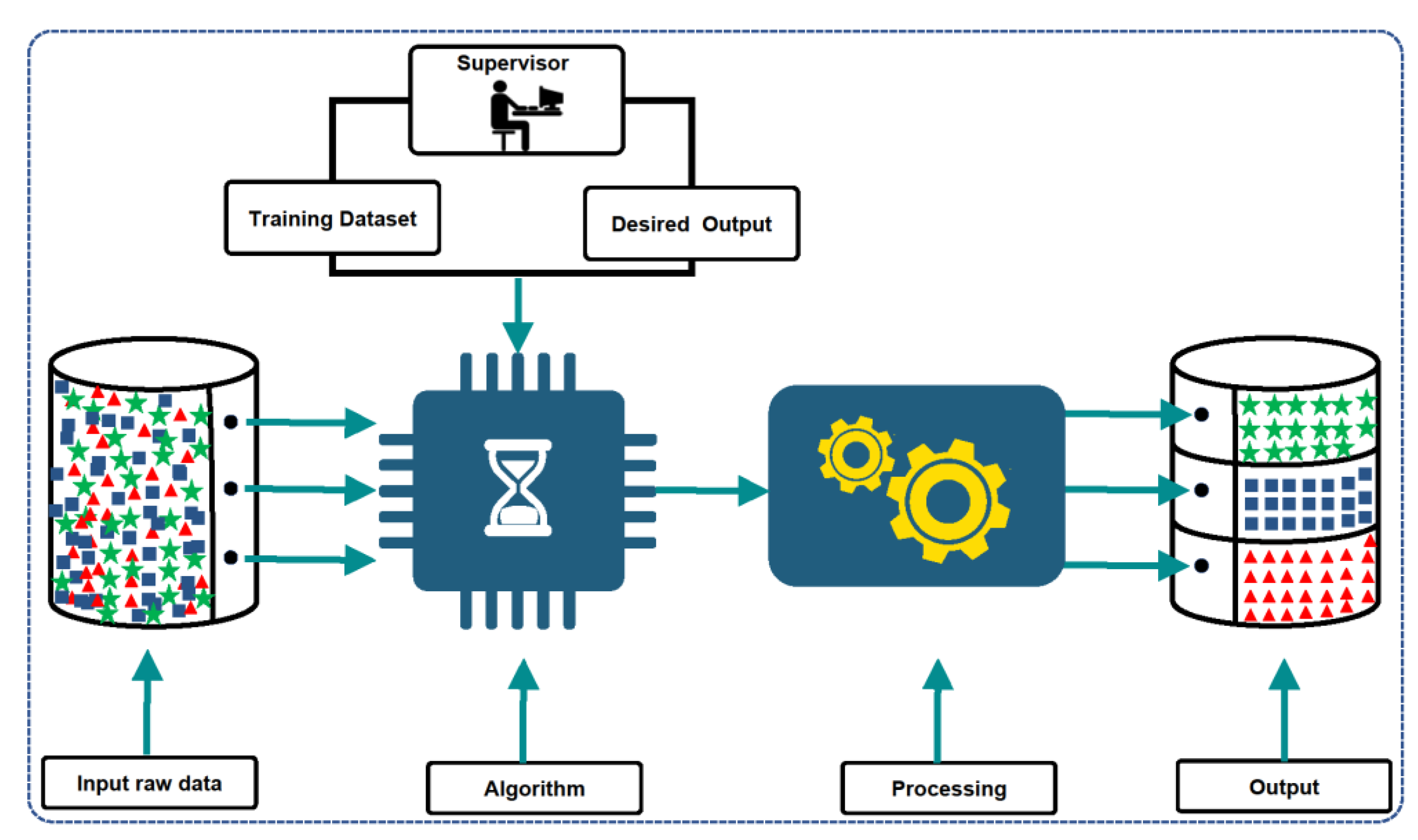As stated by [10], machine learning algorithms can be classified into three major types: supervised learning, unsupervised learning, and reinforcement learning. This research focuses mainly on supervised learning, in which the inputs are provided as a labeled dataset, from which a model is able to learn [11]. The meaning of a labeled dataset is that the desired output for each dataset is also provided. The main purpose is to learn the function of mapping the input to the desired output. Common tasks for this type of learning include classification and regression [12]. Therefore, this paper mainly emphasizes the classification task. For example, a set of samples introduced by features and consistent class labels is provided, and the classification consists of learning a model to correctly predict the class membership of each sample. Figure 1 shows how the supervised learning approach works.

As previously stated, the primary focus of this paper is the application of a feature selection approach in a classification process, as indicated by the title. Feature selection has classically been defined as a selection of k features/measurements from the original features/measurements m, (k < m), such that the value of a criterion function is optimized over all subsets of size k [13,14]. In ML tasks, feature selection is important, since most datasets contain duplicated and irrelevant features [15]. As a result, feature selection tends to reduce the dimensionality of datasets and pick the most important features to improve classification performance while decreasing computing cost [16,17,18,19]. The primary goal of feature selection is to choose a subset of features from a dataset that exhibits excellent classification performance, making it a multi-objective problem [20,21].

A multi-objective problem is a multi-criterion decision-making field that deals with optimization problems involving more than one objective function to be minimized or maximized [22]. The output is a set of solutions that describe the optimal trade-off between competing goals. The multi-objective minimization problem may be expressed mathematically as follows:

min f_k (y) = [f₁ (y), f₂ (y), …, f_i (y)]

(1)

subject to:

g_k (y) ≤ 0, i = 1, 2, …, m

(2)

h_k (y) = 0, i = 1, 2, …, l

(3)

where f_k (y) is the k-th objective that is a function of y, y is the decision variables vector, i denotes the number of objective functions to be reduced. The constraint functions are g_k (y) and h_k (y). The trade-offs between conflicting objectives highlight the superiority of multi-objective algorithm solutions. For example, the i-objective minimization problem consists of two solutions: c and d. If the following conditions are met, it can be said that c dominates d or c over d:

∀_i: f_i (c) ≤ f_i (d)  and  ∃f_i (c) < f_i (d)

(4)

when c is not dominated by any other solutions, c is referred to as a non-dominated solution.

In summary, this study proposes wrapper-based multi-objective feature selection approaches to approximate the set of Pareto optimal solutions that represents the optimum trade-off between the number of reservoir features and the classification error rate of the oil and gas reservoir recovery factor.

The remainder of the paper is divided into the following sections: Section 2 explains related studies succinctly. In Section 3, a detailed description of the proposed approaches is provided. Section 4 presents the implementation of the methodology, while Section 5 discusses the experimental results. Section 6 reports the conclusions of this study.

2. Related Work

Many studies have investigated and conducted research to determine the relationship between the recovery elements and the reservoir’s rock properties. The American Petroleum Institute (API) developed a connection between reservoir rock properties and produced fluid characteristics and oil recovery factors in 1967. For limestone, dolomite, and sandstone formations, API performed research to establish the relationship between the element of oil recovery and well spacing. Craze et al. [23] used API databases to perform an experimental analysis to explain how oil recovery is affected by the well spacing, and provided key parameters regarding the reservoir recovery variables being examined. With the exception of the greater oil/gas solution rate, Arps and Roberts [24] argue that the final recovery factor is usually proportionate to the oil gravity. To compute the recovery factor,

Gutherie et al. [25] proposed multiple similarities for sandstone reservoirs with water drive mechanisms. Because of oil retractability phenomena caused by hydrocarbon extraction, Musket et al. [26] proved that recovery factors have an inverse relationship with oil viscidity, but a direct relationship with how the gas is soluble. Instead of using experimental or theoretical evidence, API proposed several methodological associations using real field output data from the period 1957 to 1985 to calculate the recovery factors. Gulstad [27] proposed using multiple linear regression to identify the recovery factor of two types of reservoirs (sandstone and carbonate reservoirs) with or without a solution gas recovery factor. Using model-based multilinear regression, Oseh and Omotara [28] evaluated the Nigerian delta recovery factor. Similarly, a study was proposed to test the Nigerian Delta recovery factor for water-driven and depletion reservoirs [29]. Their study has some limits due to the complexity of the reservoir data.

The study in [30] performed a root-cause analysis of 145 oil and gas projects in order to investigate deficiencies in production attainment. A thorough statistical study of output achievement using a detailed worldwide database of oil and gas enterprises was performed. The findings revealed that low production was because of optimistic assumptions, failures in the assurance process, and lack of accountability for production which has led to unreliable predictions. In [31], Meddaugh reported that several key factors were the main contributors to optimistic predictions, including well location optimization workflows, areal subsurface model grid size, sparse data bias, and management bias. In [32], the authors conducted a review on how modeling workflows lead to prediction optimism and what reservoir designers, both geophysicists and scientists, could do to decrease forecast optimism obtained when using their subsurface models through a better understanding of how parameter values are used to restrict models.

Consequently, many studies have been undertaken that use AI and ML methods to better classify reservoir recovery factor. ANN, genetic algorithm (GA), support vector regression (SVR), and fuzzy logic are some of the AI/ML methods deployed [33,34,35,36]. These methods have been used in the petroleum industry to improve, discover, and quantify a variety of properties, leading to remarkable results in terms of reservoir characterization, rock identification, anomaly detection, and stranded drill pipe classification [37]. However, such approaches still suffer from problems like local optima stagnation, overfitting, and a lack of proper architectural guidance, and they have not been able to address the issue of imbalanced data [34,35,36]. The ensemble method is another viable ML approach with promising performance that has been used for oil and gas problems. The ensemble method primarily involves the mixture of at least two (weak) supervised learner algorithms to provide an aggregated (final) solution for a given classification or regression tasks. As reported by [3], for instance, an ensemble estimator model combining wavelet filters with GA in addition to the Relief method was developed to approximate the reservoir recovery factor from data obtain from a US Oil & Gas.

The work in [38] used deep learning to develop a surrogate model for recovery-factor forecasting. Based on simulation results, the performance of reservoir is dependent on fault permeability, length, and orientation, as well as undeformed reservoir permeability. With respect to recovery factor prediction, a dataset consisting of 395 Deepwater Gulf of Mexico oilfields was used to calculate dimensionless numbers [39]. In the proposed approach, principal component analysis (PCA) and K-means clustering are applied to classify oilfields. The relationship between dimensionless numbers and recovery factor is then determined by partial least square regression.

In addition, Al-Tashi et al. [37] used Binary Grey Wolf Optimizer (BGWO) as a feature selection method to select relevant features in a reservoir recovery factor problem. The proposed GWO was implemented with KNN, and its performance was compared with Binary Dragonfly Algorithm (BDA [40], and the Binary Whale Optimization algorithm (BWAO) [41]. On the basis of their experimental results, it was reported that BGWO outperformed BDA and BWAO in terms of selected features and accuracy values. However, the proposed BGWO was used as a single objective optimization approach. Formulating the selection of relevant features in reservoir recovery as a multi-objective optimization problem could select optimum features since sets of non-dominated solutions will be considered. Moreover, multi-objective optimization techniques can choose optimum features that provide better results than single-objective optimization approaches in a single run.

Consequently, this study proposes a wrapper-based multi-objective feature selection approach for selecting optimal features for reservoir recovery factor classification with a low classification error rate and a small number of reservoir features.

3. Proposed Methods

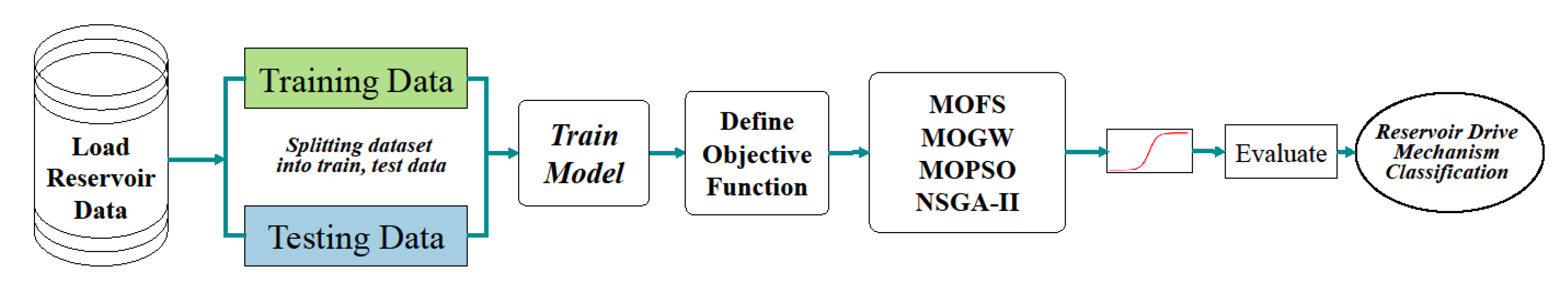
This section provides clear explanations of the proposed methods; it starts with ANN classifier used to train the models, followed by the objective function, then the multi-objective feature selection algorithms: MOGWO followed by MOPSO and the NSGA-II. This section concludes with the transfer function used to convert the search space to binary form. Figure 2 illustrates the methodology of this study. Please note that the dataset used in this study is explained in the following Section 4 Implementation of the methodology.

3.1. Artificial Neural Network Classifier (ANN)

A neural network consists of neurons organized into multiple layers, where the first layer receives an input vector and transforms it into an output vector. Each neuron takes input and applies a function to it, which is typically a non-linear function, before passing the output to the next layer. [42,43]. The network is generally meant to be feed-forward; information flows only in one direction: forward, from the input nodes to the hidden nodes (if any) and finally to the output nodes. The network has no cycles or loops [44].

An ANN classifier is used in order to compute the classification error and estimate the discrimination value for each feature. ANN has a superior computational time performance as it only needs to compute the important distances indicated by the selected feature, resulting in a reduction in the overall computational cost of the classification process [45].

3.2. Objective Function

As previously stated, while designing a multi-objective issue, there are two objectives:

• Minimizing the number of reservoir data measurements.
• Minimizing classification error rate.

The multi-objective feature selection minimization problem is expressed mathematically as follows:

$$\mathit{minimize} \mathit{OBJ}(x)=\{\begin{array}{ll}{\mathit{obj}}_1(x)=\frac{K}{M}& K\in M,M\in {ℝ}^{+}\\ {\mathit{obj}}_2(x)=\frac{FP+FN}{TP+TN+FP+FN}\times 100 & (P+N)\in {ℝ}^{+}\end{array}$$

(5)

where $M$ represents the whole measurements of a dataset while $K$ denotes the selected measurements. True positives, true negatives, false positives, and false negatives are represented by TP, TN, FP, and FN, respectively. $ob{j}_1\left(x\right)$ is the first objective, and indicates the selected measurements, while $ob{j}_2\left(x\right)$ is the second objective, representing the error rate of classification.

3.3. Multi-Objective Grey Wolf Optimizer (MOGWO)

MOGWO is a recent effective multi-objective optimizer developed by Mirjalili et al. [46], which is an extension of the original Grey Wolf Optimizer (GWO) [47], and aims to solve optimization problems with multiple objectives. Similar to GWO, MOGWO consist of four different wolves namely Alpha (α), Beta (β), Delta (δ) and Omega (ω) that form the social hierarchy of grey wolf. The best three solutions are α, β, and δ, whereas ω is the rest of solution. Mathematically, three well-designed stages that GWO obeys during the process of optimization. First, the encircling behavior was mathematically calculated as follows:

$$\overrightarrow{D}=\left|\overrightarrow{C}\times {\overrightarrow{X}}_p\left(t\right)-\overrightarrow{X}\left(t\right)\right|$$

(6)

$$\overrightarrow{X}\left(t+1\right)={\overrightarrow{X}}_p\left(t\right)+\overrightarrow{A}\times \overrightarrow{D}$$

(7)

where $t$ denotes the iteration number, $\overrightarrow{X}$ and ${\overrightarrow{X}}_p$ are two vectors that describe the wolf’s and prey’s locations, respectively, while $\overrightarrow{A}$ and $\overrightarrow{C}$ are two vectors coefficient that are given as follows:

$$\overrightarrow{A}=2\overrightarrow{a}\times \overrightarrow{r_1}-\overrightarrow{a}$$

(8)

$$\overrightarrow{C}=2\times \overrightarrow{r_2}$$

(9)

where $\overrightarrow{r_1}$ and $\overrightarrow{r_2}$ are two random vectors that can have values in the range of [0, 1], whereas $\overrightarrow{a}$ is a vector that linearly decreases over the iterative process from 2 to 0.

In addition, GWO does not change the three best solutions (α, β and δ), while it forces the other candidate solutions that belong to ω to change their positions to in order to match them. As a result, the GWO’s hunting process is performed in accordance with several equations for each candidate solution, as follows:

$$\overrightarrow{D_{\alpha }}=\left|\overrightarrow{C_1}\times {\overrightarrow{X}}_{\alpha }-\overrightarrow{X}\right|$$

(10)

$$\overrightarrow{D_{\beta }}=\left|\overrightarrow{C_2}\times {\overrightarrow{X}}_{\beta }-\overrightarrow{X}\right|$$

(11)

$$\overrightarrow{D_{\delta }}=\left|\overrightarrow{C_3}\times {\overrightarrow{X}}_{\delta }-\overrightarrow{X}\right|$$

(12)

$$\overrightarrow{X_1}=\overrightarrow{X_{\alpha }}-A_1\times \left(\overrightarrow{D_{\alpha }}\right)$$

(13)

$$\overrightarrow{X_2}=\overrightarrow{X_{\beta }}-A_2\times \left(\overrightarrow{D_{\beta }}\right)$$

(14)

$$\overrightarrow{X_3}=\overrightarrow{X_{\delta }}-A_3\times \left(\overrightarrow{D_{\delta }}\right)$$

(15)

$$\overrightarrow{X}\left(t+1\right)=\frac{\overrightarrow{X_1}+\overrightarrow{X_2}+\overrightarrow{X_3}}{3}$$

(16)

Moreover, in GWO, $\overrightarrow{a}$ represents the attacking procedure which comprises random vectors between [−a, a] that linearly decrease from 2 to 0 as the number of iterations increases. The vector $\overrightarrow{a}$ is mathematically expressed as follows:

$$\overrightarrow{a}=2-t\times \frac{2}{maxIter}$$

(17)

where $t$ is the current iteration, while $maxIter$ denotes the maximum number of iterations.

For GWO to be suitable for multi-objective problems, two new procedures were made as follows: an archive is introduced that is responsible for storing the obtained non-dominated solutions. The second procedure develops a leader selection strategy for choosing the best three solutions, represented by α, β, and δ, from the archive. Additionally, there is a controller within the archive responsible for deciding which solutions are to be saved in the archive and for controlling the archive if it becomes full. The attained non-dominant solutions are contrasted with previous representatives of the archive in each iteration. As a result, the following scenarios could be considered for an archive:

• The new solutions should not be stored in the archive if dominated by existing ones in the archive.
• Existing members in the archive should be omitted if new solutions dominate them; the new solutions will be stored instead of the omitted ones.
• In case neither solution (i.e., the existing and the new one) dominates the other, the new solutions will be stored in the archive.
• In case the archive becomes full, the grid strategy is used to omit the most crowded segment solutions that are stored in the archive and insert the new solutions.

On the basis of the concept of the Pareto front, solutions cannot be easily compared; therefore, a leader selection technique is proposed to solve this problem. In GWO, the best three solutions, represented by α, β, and δ, act as leaders to guide other search agents towards promising regions that can lead to better solutions and converge to the global optimal solution. The leader selection selects the smallest crowded portion of the searching space and offers one of its non-dominated solutions such as α, β, or δ wolves.

The selection procedure is performed using the roulette-wheel method according to the likelihood for hypercubes, as given in the following:

$$P_j=\frac{m}{H_j}$$

(18)

where $m$ is a constant that can have a value more than one while $H$ represents the total number of gained Pareto front in the jth segment.

3.4. Multi-Objective Particle Swarm Optimization (MOPSO)

The concept of the MOPSO algorithm is to have a global repository where each particle deposits its flight experiences after completion of a flight cycle [48]. Moreover, the fitness values of each particle build a geographical system that helps to update the repository. Particles use the repository to select a leader that is responsible for guiding the search, where each particle may select a different leader. The algorithm strategies rely on hypercubes that can be produced by splitting the explored search space. The following presents the MOPSO Algorithm 1:

Algorithm 1 MOPSO Algorithm

Initialize the population N, and the velocity of all particles (set to zero initially). Evaluate the fitness of all particles in POP. Particles positions which denote non dominant vectors in the repository represented by REP are stored. Generate hypercubes of the searching space that has been explored so far. Using the generated hypercubes, locate the coordinates of particles where their finesses form a coordinate system. Initialize the history of all particles and store it in REP. whilet < maximum number of cycles do For i = 1: N (a) Calculate the velocity based on Equation (19). (b) Update the position of all particles: N[i] = N[i] + V[ i] End for (c) Maintain the particulate matter inside the search area if it goes past its limits (generating solutions that are out of search space are not considered). (d) Evaluate the fitness of all particles. (e) The contents of REP and the geographical representations of the hypercubic particles are updated including removing dominant sites from the archive. In addition, unreported places are added. Until the size of the archive is complete, a high priority is given to particles located in less crowded target areas over particles that reside in densely populated regions. (f) In case a particle position is greater than its previous position, its position changes as follows: The criterion for determining the location from memory is precisely that Pareto superiority should be applied The position in memory is kept in case the current position is dominated by the position in memory, else the position in the memry is replaced by the current position. In case none of the current position or the position in momery dominates the other, then one of them is selected randomly. (g) t = t + 1.   END WHILE

The following expression shows the computation speed of particle $i$:

V[i] = W × V[i] + R1 × (PBESTS[i] − N[i]) + R2 × (REP[h] − N[i])

(19)

where $w$ denotes the inertia weight that has a value of 0.4. R1 and R2 are two numbers generated with a random distribution in the range of [0, 1]. PBES[i] denotes the best historical position of particle $i$. REP[h] is a taken value from the repository where h is selected based on the following: hypercubes that have more than one particle are equivalent to the division of any number z > 1 (in this work, z = 10) by the population size in it. This procedure attempts to reduce the fitness of these hypercubes which can generate additional particles and as illustrated in [5], this approach is a one way of fitness sharing [5]. To select hypercube where the relevant particle is taken, the roulette wheel selection method is implemented. After hypercube selection, a particle is chosen randomly. The value of particle $i$ is denoted as N[i].

3.5. Non-Dominated Sorting Genetic Algorithm II (NSGA-II)

According to [49], due to its quick non-dominated trial, simple congested comparison operator, and fast overcrowded distance valuation, NSGA-II can be considered to be one of the most prominent optimization algorithms, efficiently solving problems with multiple objectives. The work in [50] implemented the NSGA-II approach, and it was shown that NSGA-II outperforms PAES and SPEA in obtaining diverse solutions. Generally, the steps of NSGA-II are described as follows:

• Step 1: Initialize the population based on limitation and the issue.
• Step 2: Non-domination sort
  Sorting is performed with a focus on population non-dominance criterion.
• Step 3: Crowd distance
  After the sorting step, assigning crowding distance is performed. Individuals are chosen according to their crowding distance and ranking.
• Step 4: Selection
  A binary selection tournament is applied along with crowded-comparison operator in order to select individuals.
• Step 5: Crossover and mutation of real coded GA are implemented.
• Step 6: Recombination and selection
  Current population and offspring population are merged together. The population of next generation is selected, and it is filled till the size of its population is more than the size of the current population.

3.6. Transfer Function

Initially, MOGWO and MOPSO were suggested to solve continuous optimization problems. The problems of multi-objective feature selection cannot be explicitly addressed. The search space needs to be transferred from continuous into a binary one, so the algorithms suit the nature of feature selection.

The search space bounds for feature selection are 0 and 1, indicating that feature selection is a binary dilemma. Using original MOGWO and MOPSO to handle the feature selection dilemma is not an option. As a result, it is crucial to develop a binary version of MOGWO. The transfer function in (20) is introduced to convert the positions of search candidates for the MOGWO and MOPSO algorithms to a binary search space [51,52]:

$$S\left(x\right)=\frac{1}{1+{\mathrm{e}}^{\left(-10\ast \left(x-0.5\right)\right)}}$$

(20)

4. Implementation of the Methodology

This section describes the dataset used to implement this study as well as the parameter settings of the multi-objective algorithms.

4.1. Dataset

The experimental data used in this investigation were obtained from the literature [3,23,27]. As shown in

Table 1. Reservoir class types [3,23,27].

Class Label	Reservoir Class	#Data Samples
0	Sandstone reservoirs (Water drive)	128 samples
1	Carbonate reservoirs (Water drive)	30 samples
2	Sandstone reservoirs (Solution gas drive)	139 samples
3	Carbonate reservoirs (Solution gas drive)	70 samples

, the dataset contains 367 sandstone and carbonate lithology primitive reservoirs, of which 209 reservoirs are driven by dissolved gas and 158 reservoirs are driven by water. As a result, Table 1 illustrates the study’s target class.

Table 2. Measurements of the reservoir [3,23,27].

	Measurement Name	Abbreviation
1	Bo at initial pressure	Boi
2	Rock permeability to air	K
3	k/Uob ratio	k/Uob
4	Temperature	T
5	Oil Formation Volume Factor	Bo
6	Oil viscosity at initial pressure	Uoi
7	Water viscosity	Uw
8	Oil Formation Volume Factor at abandonment pressure	Boa
9	Pressure at the end of Primary	Pep
10	Oil viscosity at bubble point	Ubp
11	Solution gas ratio at bubble point	Rsb
12	Oil viscosity at Abandonment pressure	Uoa
13	Solution gas ratio at abandonment pressure	Rsa
14	Net pay thickness	h
15	Effective Porosity	Por
16	Connate water saturation	Sw
17	Initial reservoir pressure	Pi
18	Solution gas ratio at initial reservoir pressure	Rsi
19	Bo at bubble point pressure	Bob
20	Oil Gravity	API
21	Calculated (OOIPcal)	OOIPcal
22	Pressure ratio	Pb/Pa
23	Original-oil-in-place at initial pressure as reported by the operator	OOIP

indicates that 23 reservoir measurements were used as input data for determining the reservoir’s recovery factor. As a result, the input data used in this study were actual data performance from oil and gas fields in the United States. These input data/measurements were acquired via well logs, core analyses, sensors, and drill stem tests performed during real-world operations.

4.2. Parameter Settings

This subsection describes the parameter settings of the three approaches; the dataset was divided into two sets at random: training (70%); and testing and validation (30%). With a random seed, all algorithms were executed 10 times using the MATLAB 2017a platform. The ANN classifier was configured with 10 hidden layers and a learning rate of 0.8. The three algorithms used in this study are wrapper-based techniques, which need the use of a classifier for evaluating the classification error for the measure chosen during the training evolutionary phase.

Table 3. Parameter setting of the three multi-objective algorithms.

Parameter	MOGWO	MOPSO	NSGA-II
Max Iteration	100	100	100
Number of Populations	50	50	50
Storage Capacity	100	100	100
Alpha	1.5	1.5	-
Beta	2	2	-
Gamma	4	4;	-
nGrid	20	20	-
c1	-	1;	-
Wdamp	-	0.99;	-
c2	-	2;	-
W	-	0.5;	-
pMutation	-	-	=0.4;
Mu	-	0.1;	0.1;
nMutation	-	-	Round (pMutation *nPop);
pCrossover	-	-	0.9
nCrossover	-	-	2 *round (pCrossover *nPop/2);

presents the parameter settings of the three algorithms.

5. Results and Discussion

This section presents the results and comparison of the three algorithms, as well as the discussion.

5.1. Experimental Results

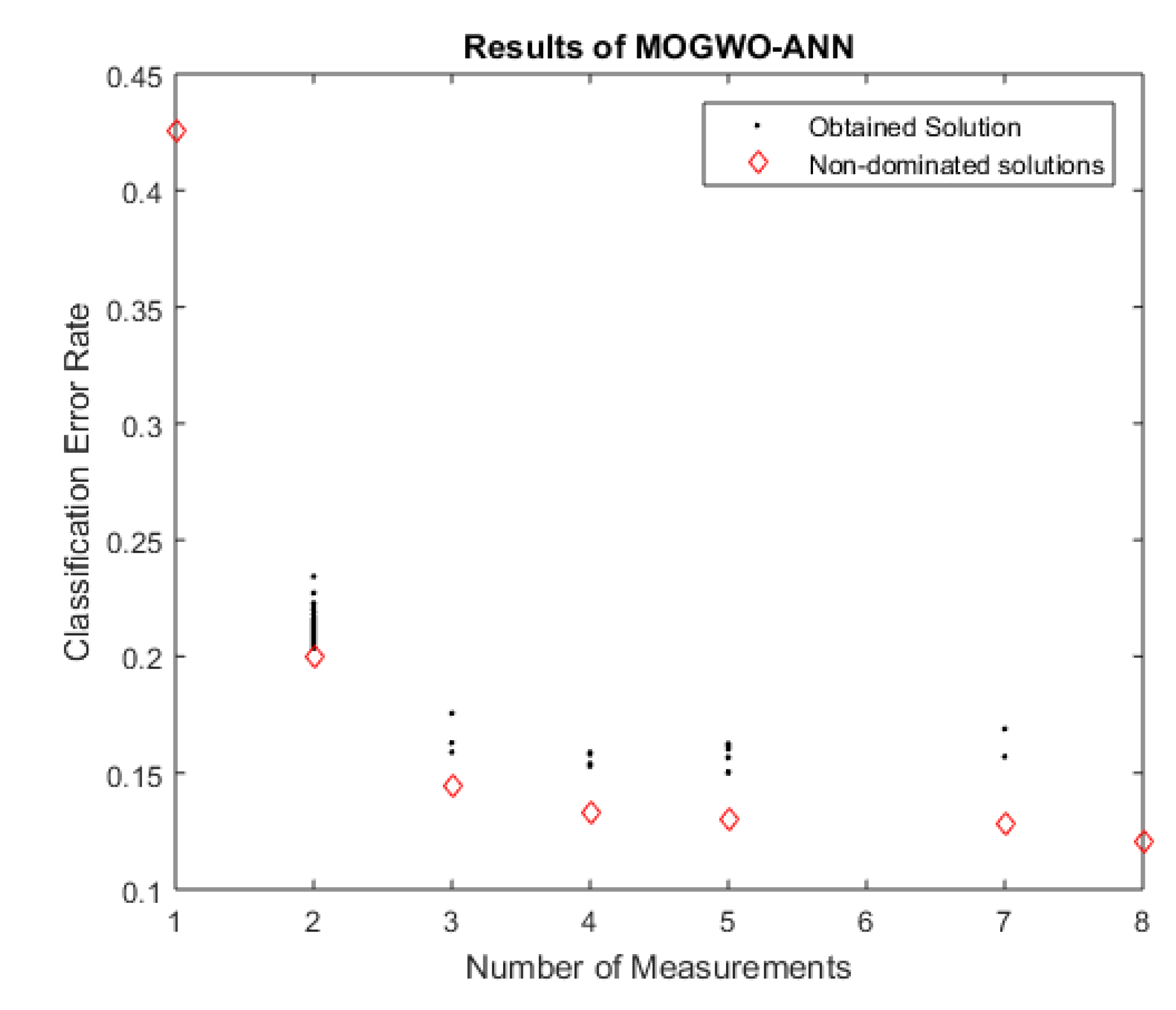
This subsection presents the obtained results for the three proposed approaches. It starts first with the proposed MOGWO-ANN. As can be seen from Figure 3, the x-axis represents the number of measurements while the error rate of classification is on the y-axis. Figure 3 illustrates that the MOGWO-ANN produced seven non-dominated solutions that efficiently selected fewer measurements and obtained a lower error rate with respect to classification than using all original features, where the error rate using the original feature was 0.229. The proposed MOGWO-ANN selected approximately 40% from the original features (8 from 23). A clear detail of the produced non-dominated solutions is shown in

Table 4. Results of the MOGWO-ANN.

#No of Solutions	#No Selected Features	Error Rate	Measurements Selected
1	8	0.120	h, API, Pep, Uoa, Uw, Bob, OOIP and OOIPcal
2	7	0.128	API, Pep, Uoa, Uw, Bob, OOIP and OOIPcal
3	1	0.425	Bob
4	5	0.130	h, API, Bob, OOIP and OOIPcal
5	2	0.199	Bob and OOIP
6	4	0.133	Pep, Bob, OOIP and OOIPcal
7	3	0.143	Bob, OOIP and OOIPcal

, where the best attained result in solution 1 with a lower classification error rate of 0.120 and a small number of measurements, with the eight most critical measurements of the reservoir heavily contributing to the accurate classification of the reservoir recovery factor which are (h, API, Pep, Uoa, Uw, Bob, OOIP and OOIPcal).

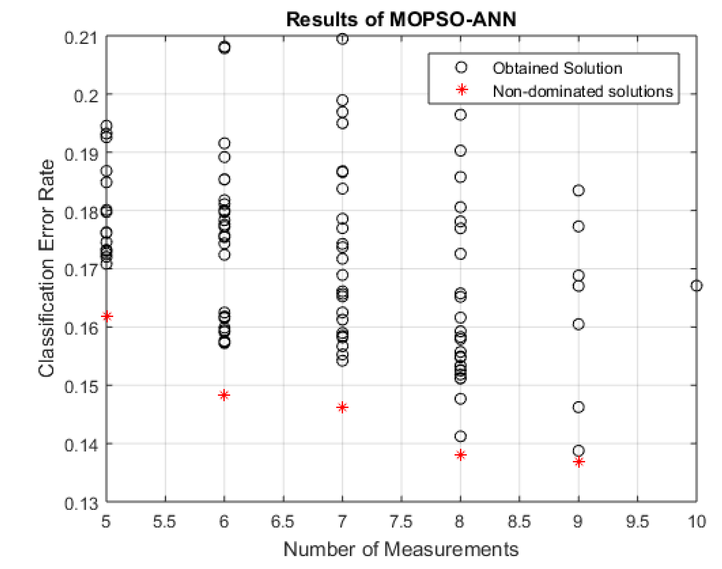
Secondly, the MOPSO-ANN approach. As can be seen from Figure 3, the horizontal axis and the vertical axis represent the number of measurements and the error rate of classification, respectively. Figure 4 shows that the MOPSO-ANN produced five non-dominated solution which are efficiently able to select fewer measurements and obtain a less error rate of classification than using all original features, where the error rate using the original feature is 0.229. MOPSO-ANN selected nine features from the original 23 features, which is approximately 45%. A clear detail of the produced non-dominated solutions is shown in

Table 5. Results of the MOPSO-ANN.

#No of Solutions	#No Selected Features	Error Rate	Measurements Selected
1	6	0.148	Sw, PI, Pep, Uoi, Bob and OOIP
2	5	0.162	Sw, Pep, Uoi, Bob and OOIP
3	8	0.138	Sw, API, PI, Pep, Uoi, Rsa, Bob and OOIP
4	9	0.136	k/uob, Sw, PI, Pep, Uoi, Rsa, Bob, Bol and OOIP
5	7	0.146	Sw, PI, Pep, Uoi, Rsa, Bob and OOIP

, where the best obtained result in solution 4 with less classification error rate of 0.136 and small number of measurements with 9 most critical measurements of the reservoir that contribute to accurate classification of the reservoir recovery factor which are (k/uob, Sw, PI, Pep, Uoi, Rsa, Bob, Bol and OOIP).

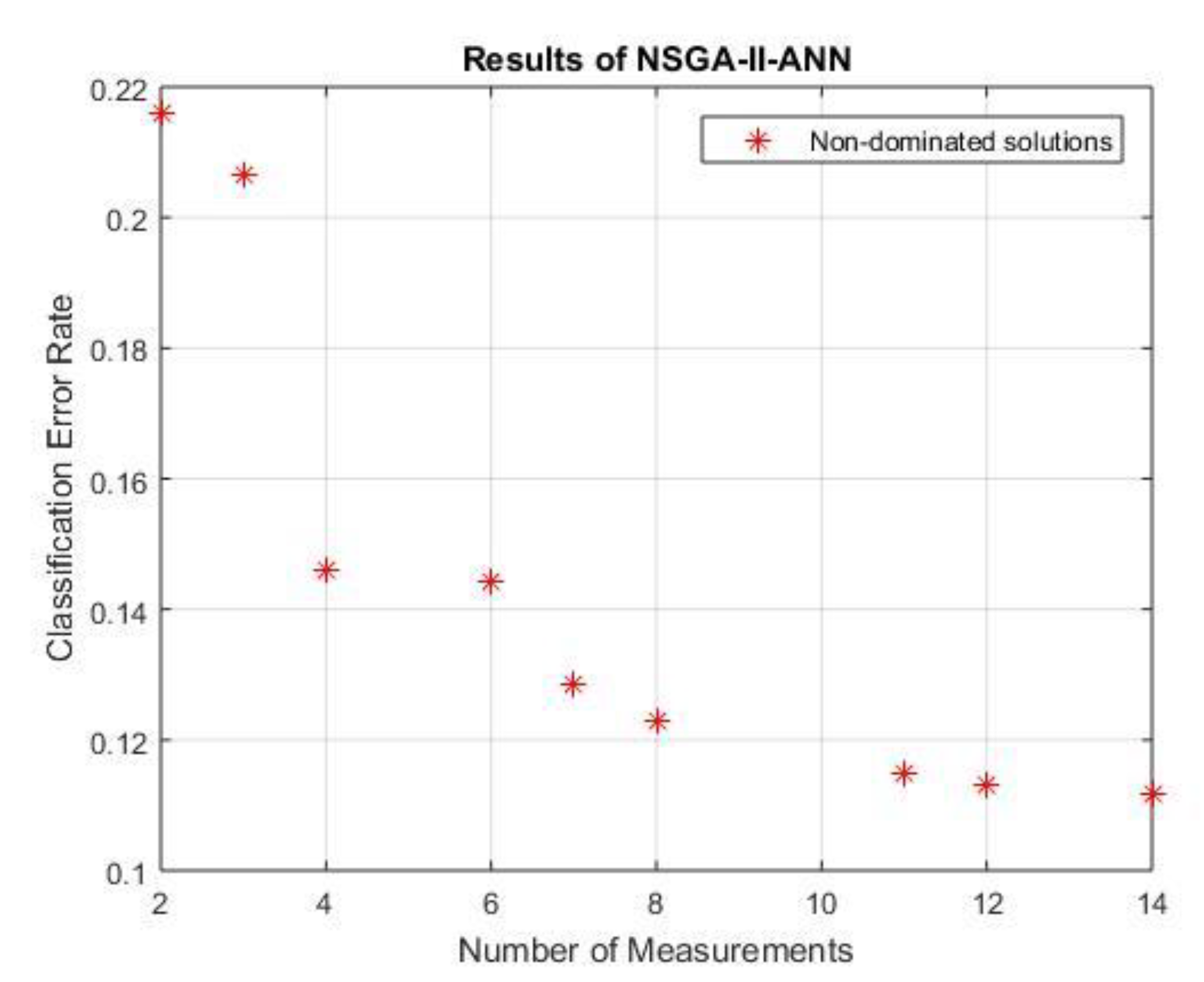
Lastly, the NSGAII-ANN approach. As can be seen from Figure 4, the horizontal axis and the vertical axis represent the number of measurements and the error rate of classification, respectively. Figure 5 shows that NSGAII-ANN produces nine non-dominated solution which efficiently can select fewer measurements and obtain a less error rate of classification than using all original features, where the error rate using the original feature is 0.229. MOPSO-ANN selected 14 features from the original 23 features, which is approximately 55%. A clear detail of the produced non-dominated solutions is shown in

Table 6. Results of the NSGAII-ANN.

#No of Solutions	#No Selected Features	Error Rate	Measurements Selected
1	2	0.216	Bob and OOIP
2	14	0.112	h, Sw, T, API, PI, Pep, Pb/Pa, Uoa, Rsb, Rsa, Bob, Boa, OOIP and OOIPcal
3	4	0.145	Pep, Bob, OOIP and OOIPcal
4	3	0.206	Uw, Bob and OOIP
5	8	0.123	Sw, PI, Bp, Pep, Bob, Boa, OOIP and OOIPcal
6	11	0.115	Por, k/uob, Sw, PI, Pep, Uw, Rsi, Bob, Boa, OOIP and OOIPcal
7	6	0.144	Sw, T, Pep, Bob, OOIP and OOIPcal
8	7	0.128	PI, Pep, Rsi, Bo, Bob, Boa and OOIP
9	12	0.113	Sw, T, API, Pep, Pb/Pa, Uoi, Uoa, Rsa, Bob, Boa, OOIP and OOIPcal

, where the best obtained result in solution 2 with a lower classification error rate of 0.112 and the 14 most critical measurements of the reservoir contributing to the accurate classification of the reservoir recovery factor, which are (h, Sw, T, API, PI, Pep, Pb/Pa, Uoa, Rsb, Rsa, Bob, Boa, OOIP and OOIPcal).

5.2. Comparison of Algorithms

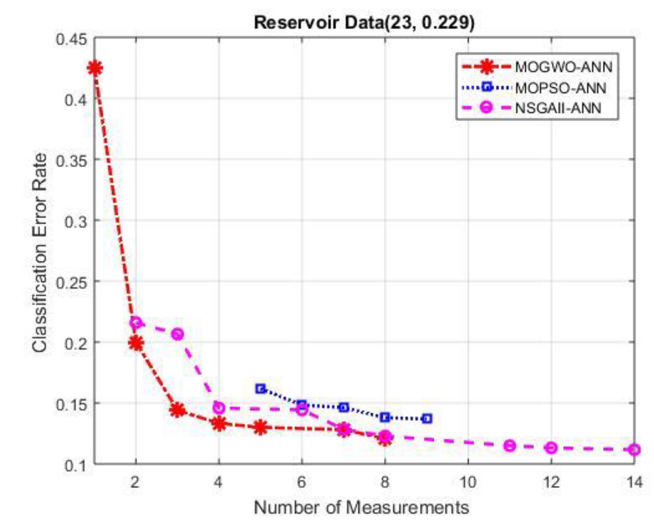
In this subsection, the three algorithms were compared against each other in order to clearly state which method perform best. As can be seen from Figure 6, the reservoir data, the error rate, and the number of measurements using all measurements are illustrated above the graph. The number of measurements chosen is shown by the x axis, while the classification error rate is represented by the y axis. The one in red color represents MOGWO-ANN approach, blue color represents MOPSO-ANN, and the cyan color indicates the NSGAII-ANN.

As illustrated in Figure 6, the MOGWO-ANN approach attained better results than both the MOPSO-ANN and NSGAII-ANN methods, both in number of measurements and the obtained error rate. It produced seven solutions, seven of them have less error rate compared to the error rate of the original measurements. Additionally, it outperforms both NSGAII-ANN and MOPSO-ANN in terms of the reduction of measurement and error rate. Nevertheless, MOGWO-ANN produced one solution contains only one measurement with high error rate, which is normal. NSGAII-ANN produced nine solutions which also good in terms of error rate compared to the one of the original measurements. However, it comprises more measurements compared to MOGWO-ANN and MOPSO-ANN. The MOPSO-ANN produced five solutions only, with a lower error rate compared to the error rate of the original data. Nevertheless, the error rate obtained by MOPSO-ANN is worse in most cases compared to NSGAII-ANN and MOGWO-ANN.

A further comparison was performed among the statistical results of for number of selected measurements obtained by MOGWO-ANN, MOPSO-ANN and NSGAII-ANN. First, it is obviously shown in

Table 7. Results of the statistical analysis on the number of selected measurements.

Measures	MOGWO-ANN	MOPSO-ANN	NSGAII-ANN
Min	1	5	2
Max	8	9	14
Range	7	4	13
STD	2.56	1.58	4.19
Average	4.29	7	7.45
Computational Time/Minutes	109	150.84	127.84

that MOGWO-ANN attains the smallest average number of measurements with the average of 4.29, compared to MOPSO-ANN and NSGAII-ANN, with averages of 7 and 7.45 measurements, respectively.

Similarly, in terms of minimum selected measurements, maximum selected measurements as well as the computational time spent, in most cases the MOGWO-ANN obviously outperforms the benchmarking methods MOPSO-ANN and NSGAII-ANN. In terms of the range between the minimum and maximum selected measurements as well as standard division the MOPSO-ANN outperformed the other two approaches. In summary in most cases the MOGWO-ANN approaches dominates both NSGAII-ANN, as well as MOPSO-ANN, especially in terms of the reduction of measurements as well as the computational time. This is due to the unique properties that MOGWO owns such as the same number of parameters as well as the small memory size it requires. A complete discussion is provided in the next section.

5.3. Discussion

The findings demonstrated that MOGWO-ANN outperforms the other two algorithms in most cases. This is due to the fact that MOGWO employed a variety of strategies to keep the selection of wolf leader diverse. It also contains a regulator that regulates which solutions are saved in the archive and nominate the leader that is in charge of selecting the best option to maintain the variety of the wolves and protect them from being imprisoned in local areas, the algorithm’s unique properties, which allow it to maintain the balance of two essential elements, exploration and exploitation, resulting in the escape of being trapped in local optima. Having fewer parameters is another benefit of this approach over others. Furthermore, it requires a minimal amount of memory as a result of having a single position vector that is more useful for big datasets in the matter of time consuming, whereas MOPSO has the vectors of position and velocity. In addition, the leader selection mechanism selects the less congested part of the search area and presents one of the non-dominant solutions, such as alpha, beta, or delta wolves, that are temporarily omitted so that selecting the same solutions is prevented, and then when the maximum iteration is finished, the optimal solutions are archived as non-dominated solutions.

Moreover, a further component is that the gird technique, which is accountable for omitting the existing solution once the archive becomes full and adding a better solution, whereas MOPSO stores the previously found solutions, resulting in repeated solutions, which is the main cause of the issue of premature convergence. Correspondingly, the NSGA-II used an identical method to store non-dominated solutions. The NSGA-II additionally implements different strategies such as mutation, which may greatly impact the search. Choosing only one solution from the acquired non-dominated solution, on the other hand, is regarded as a serious challenge. In the problem of feature selection, there are two competing aims: a trade-off between reducing feature subsets and optimizing classification performance when choosing among them.

6. Conclusions

A multi-objective feature selection approach based on three algorithms, namely, MOGWO, MOPSO and NSGA-II, was proposed for the classification of reservoir recovery factor. The ANN classifier was applied to assess the goodness of the selected features and sigmoid transfer function employed to transmit the search space into a discrete one to satisfy the feature selection condition. The findings showed that MOGWO-ANN produced better results compared to the other two algorithms in terms of reducing the number of measurements, the error rate, and the computational time. The following summarizes the major contributions of this work:

• Multi-objective optimization algorithms have efficiently addressed complex reservoir data and accurately classified the reservoir recovery factor.
• Eight significant reservoir measurements that contribute to recovery factor were identified by MOGWO-ANN, namely k/uob, Sw, PI, Pep, Uoi, Rsa, Bob, Bol and OOIP.
• In this research, MOGWO-ANN was considered to be the best approach for choosing the most useful measurements of the U.S.A. reservoir data.

The multi-objective feature selection approaches in this research are essential for dealing with the oil and gas domain to identify informative measurements with high classification performance. For future work, other oil and gas big data will be investigated as well other multi-objective optimizations algorithms such as multi-objective whale optimization algorithm, multi-objective arithmetic optimization algorithm could be used. Additionally, different classifiers could be used to assist the selected measurements.