Article

Influence of Pile Diameter and Aspect Ratio on the Lateral Response of Monopiles in Sand with Different Relative Densities

1
College of Civil Engineering and Architecture, Zhejiang University, Hangzhou 310058, China
2
Faculty of Civil Engineering and Geosciences, Delft University of Technology, 2628CD Delft, The Netherlands
3
Key Laboratory of Offshore Geotechnics and Material of Zhejiang Province, Hangzhou 310058, China
4
Key Laboratory for Far-Shore Wind Power Technology of Zhejiang Province, Power China Huadong Engineering Corporation Limited, Hangzhou 311122, China
5
Construction Management Department, Zhejiang Province Energy Group Company Ltd., Hangzhou 310007, China
*
Author to whom correspondence should be addressed.
J. Mar. Sci. Eng. 2021, 9(6), 618; https://doi.org/10.3390/jmse9060618
Submission received: 10 May 2021 / Revised: 29 May 2021 / Accepted: 31 May 2021 / Published: 3 June 2021
(This article belongs to the Special Issue Instability and Failure of Subsea Structures)

Abstract

:
The large-diameter monopiles are the most preferred foundation used in offshore wind farms. However, the influence of pile diameter and aspect ratio on the lateral bearing behavior of monopiles in sand with different relative densities has not been systematically studied. This study presents a series of well-calibrated finite-element (FE) analyses using an advanced state dependent constitutive model. The FE model was first validated against the centrifuge tests on the large-diameter monopiles. Parametric studies were performed on rigid piles with different diameters (D = 4–10 m) and aspect ratios (L/D = 3–7.5) under a wide range of loading heights (e = 5–100 m) in sands with different relative densities (Dr = 40%, 65%, 80%). The API and PISA p-y models were systematically compared and evaluated against the FE simulation results. The numerical results revealed a rigid rotation failure mechanism of the rigid pile, which is independent of pile diameter and aspect ratio. The computed soil pressure coefficient (K = p/Dσ′v) of different diameter piles at same rotation is a function of z/L (z is depth) rather than z/D. The force–moment diagrams at different deflections were quantified in sands of different relative density. Based on the observed pile–soil interaction mechanism, a simple design model was proposed to calculate the combined capacity of rigid piles.

1. Introduction

The offshore wind energy has achieved significant development in recent years with a global installation of 31.9 GW by the end of 2020 compared with 3.3 GW in 2011 [1]. Currently, in shallow waters with depth of less than 40 m, the monopiles are the most widely used foundation type for supporting OWTs, accounting for more than 87% of all installations in Europe [2]. The monopile foundations used in offshore wind farms usually have a diameter (D) larger than 6 m, but aspect ratio (L/D, L is embedded length) much less than 8 [3,4,5,6]. Meanwhile, monopiles with diameter larger than 10 m are under consideration for the larger capacity OWT in deeper waters [7]. These large-diameter short monopiles exhibit a rigid pile behavior under lateral loading [8].
The OWTs are subjected to combined horizontal force and overturning moment simultaneously from the actions of wind, wave and currents. The equivalent loading eccentricity of horizontal force can reach 2.5L (L is pile embedded length) above the ground surface [9,10]. The combined load-bearing behavior of large-diameter rigid piles is one of the most crucial factors in the foundation design of OWTs. Among all the existing analysis methods, the p-y method is still the most widely used one for the laterally loaded monopile due to its simplicity and high efficiency. In this method, the monopile is modelled by the beam elements while the soil is represented by a series of nonlinear springs distributed along the pile length. During past decades, many p-y models have been proposed for the laterally loaded pile in sand, including (but not limited to) Reese et al. [11], Bogard and Matlock [12], O’Neill and Murchison [13], Georgiadis et al. [14], Klinkvort [15], Kirkwood [16], Zhu et al. [17], Wang et al. [18], Suryasentana and Lehane [19], Suryasentana and Lehane [20], etc. Of all the existing p-y models, the ones proposed by Reese et al. [11], Bogard and Matlock [12] and O’Neill and Murchison [13] share the same root, being based on the same field tests on the small diameter flexible piles in very dense sand. The version proposed by O’Neill and Murchison [13] was adopted by the API code [21] and has been used in the pile design of oil and gas platform for decades. The API p-y model was also directly used in the initial age of offshore wind farm design. However, it was found that the API p-y model is not suitable for the design of large-diameter monopiles [3]. Experimental results in Georgiadis et al. [14], Klinkvort [15], Kirkwood [16], Zhu et al. [17] and Wang et al. [18] all suggested a significant overestimation of lateral pile stiffness from the API p-y model. Lam and Martin [22] and Ashour and Helal [23] argue that the additional resistance provided by the base shear, base moment and the shaft friction in addition to the p-y curves should be considered for the rigid pile. Inspired by Lam and Martin [22] and Ashour and Helal [23], Byrne et al. [24] proposed a four-spring model to incorporate all the components based on a series of field tests and numerical simulations. A completely new form of p-y models was proposed for the rigid pile [25]. However, it should be noted that numerical [25] and field test [8] results suggested that the influence of pile base is less than 10% for most cases. The response of monopile is still mainly controlled by the p-y curves. Although new p-y models have been proposed, no systematic studies have been carried out to discuss the difference and evaluate the performance against the API p-y models.
Apart from the p-y method, FE modelling has been used more in analyzing the lateral bearing behavior of monopiles due to the development of computation power and soil modelling. Numerical simulations on the monopile under lateral loading have been performed by Achmus et al. [26], Achmus et al. [27], Thieken et al. [28] and Ahmed and Hawlader [29]. Same overestimation of pile response by API p-y models was reported for the large-diameter monopile. However, most of the existing numerical studies were performed using an elasto-perfect plastic model with Mohr–Coulomb failure criteria. The state-dependent behavior of sand with different relative densities cannot be modelled.
Up to date, no systematic studies have been conducted to quantify the combined lateral bearing capacity of large-diameter monopiles with different diameters and aspect ratios in sands with different relative densities. Nor have the difference and performance of existing p-y models been discussed and evaluated. This study presents a comprehensive three-dimensional finite element (FE) study on the lateral bearing behavior large diameter monopiles in sands with three different relative densities (Dr = 40%, 65%, 80%). To model the nonlinear, state-dependent behavior of sand, an advanced hypoplastic model was adopted. The FE model was first validated against the centrifuge tests of large-diameter monopiles in sand. A wide range of pile diameters (D = 4, 6, 8, 10 m), aspect ratios (L/D = 3, 3.75, 5, 7.5) and loading eccentricities (e = 5, 10, 20, 40, 60, 80, 100 m) were investigated using the validated FE model. The traditional p-y model in API from small-diameter flexible pile and that newly proposed by Burd et al. [25] for large-diameter monopile were systematically compared and evaluated. The combined force–moment capacities of monopiles under different deflection criterion in sands with different relative density were also quantified. A simple model based on the soil pressure distribution along the rigid pile is also proposed to calculate the combined capacity of monopiles.

2. Discussion on the Existing p-y Models

The p-y model in API was originally proposed based on field tests of small-diameter flexible piles and mainly used for the design of long flexible piles in oil and gas industry. On the contrary, the p-y model proposed by Burd et al. [25] is part of the output from the most recent research of the PISA project based on the field tests and numerical simulations on large-diameter short monopiles. The model is proposed specifically for the monopile used in offshore wind farms. Therefore, before looking into the simulation results from FE modelling, it is worth first discussing and comparing the two p-y models in API [21] and Burd et al. [25].
Table 1 presents the formulation and model parameter definition of the p-y models in API [21] and Burd et al. [25]. As shown in the table, the p-y model in API adopts a tangent hyperbolic function as the backbone function. Two model parameters are required to define the p-y curves, i.e., the initial stiffness coefficient k and the ultimate resistance pu corrected by the depth factor A. It can be seen that the stiffness coefficient k and soil resistance pu is only function of soil friction angle. As a result, the initial stiffness of p-y curves increases linearly with depth. Meanwhile, as shown in the table, there is a sudden change of pu and A at a certain depth as depth increases. The ultimate resistance “Apu” will be a function of z/D, meaning that the soil pressure p/D of different diameter piles at same depth z will be different. Compared with the API p-y model, the p-y model proposed by Burd et al. [25] from the PISA project employs a four-parameter conic function as the backbone function. Each of the four model parameters (k, pu, yu, n) has a straightforward interpretation, where the parameter k controls the initial slope, pu is the ultimate value of the normalized soil reaction, yu is the required normalized displacement to mobilize the ultimate value of soil reaction. The parameter n (0 ≤ n ≤ 1) controls the nonlinear transition part between the initial and the ultimate. Instead of soil friction angle, the model parameters of the PISA p-y model are defined in terms of soil relative density. It should be noted that the model parameters in Table 1 were proposed based on the numerical simulations validated against the field tests performed in a dense marine sand at Dunkirk [10].
To directly compare the p-y models in API [21] and Burd et al. [25], p-y curves at different depths of typical large diameter monopiles in medium dense sand (Dr = 65%) were calculated and are presented in Figure 1. Figure 1a shows the normalized p/Dσv-y/D curves of different diameter piles at the depth of 2D below the ground surface. As shown in the figure, the API p-y model gives the same normalized curves for all the diameter monopiles, suggesting that the p-y curve is defined in terms of the depth ratio z/D. On the contrary, the p-y curves calculated from PISA model are different for different diameter monopiles. This is because that the p-y curves in the PISA model are defined in terms of depth ratio z/L, as shown in Table 1. Therefore, although the z/D ratios of p-y curves in Figure 1a are same, the z/L ratios are different due to the change of pile diameter. When calculating the p-y curves at the same depth of 5 m, as shown in Figure 1b, the p-y curves in PISA model all converged with each other compared with the API p-y model.
To further elaborate the difference between the p-y model in API [21] and Burd et al. [25], the normalized ultimate soil resistance profile of different diameter monopiles were plotted in Figure 2 in two different ways. As shown in Figure 2a, the normalized soil resistance profiles calculated from API converged against the depth ratio z/D, when different distributions are observed for different diameter monopiles using PISA p-y model. However, when replotting the profiles against the depth ratio z/L in Figure 2b, the profiles calculated by PISA p-y model converged into a single line.
The comparison and discussion on the API [21] and Burd et al. [25] p-y models suggested that not only the backbone formulations are different, but also the definition of p-y curves relative to the depth in the two models are also completely different. It is therefore worth evaluating the performance of the two models for modelling the lateral behavior of large-diameter monopiles.

3. Three-Dimensional Finite Element Modelling

3.1. FE Model Mesh

The three-dimensional finite element (FE) models of large-diameter monopiles were developed in the finite element program Abaqus [30] and employed for parametric studies. A series of numerical simulations were performed on monopiles with different diameters (D = 4, 6, 8, 10 m). The same embedded length (L) of 30 m was used for all the piles, meaning that the aspect ratio of simulated monopiles varies from 3 to 7.5. The pile diameter and aspect ratio in this study have covered almost all cases of monopiles in the existing or planned offshore wind farms. The OWTs are subjected to the combined loads of large overturning moment and horizontal force from wind, wave and currents. The applied load can be simplified as a horizontal force acting at certain loading eccentricity (e). According to McAdam et al. [10] and Richards et al. [9], the equivalent loading eccentricity of horizontal force can be as large as 2.5L.
To quantify the loading bearing behavior of large-diameter monopiles under different load conditions, simulations under seven different loading eccentricities of 5 m, 10 m, 20 m, 40 m, 60 m, 80 m and 100 m (e = 0.167–3.33L) were performed for each monopile. Details of simulations are summarized in Table 2.
A typical model mesh of the monopile with a diameter of 10 m and an embedded length of 30 m is presented in Figure 3. The lateral force was applied at 5 m above the ground surface. Considering the symmetry of the problem, only half of the pile–soil system was modelled to save the computation time. The horizontal boundaries of the model were simulated by a roller support, while the bottom boundary was fixed in all directions. The numerical model has a diameter of 20D and a depth of 4D beneath the pile tip. It was found that the change of load-deflection response from doubling the model dimension and mesh density is less than 1%. The monopile and sand were both modelled with eight-node linear strain brick elements (i.e., C3D8). The monopiles were modelled as rigid body by assigning a high elastic stiffness. The monopile–soil interface behavior is modelled using full 3D, zero-thickness following a classical Coulomb interface model. In the model, the tangential frictional stress is linearly proportional to the normal stress by a frictional coefficient. An interface friction angle δ of 2/3 φ (where φ denotes internal friction angle) is used in this study [31,32].

3.2. Sand Constitutive Model and Model Parameters

The advanced hypoplastic model for sand is used in this study to model the nonlinear, state-dependent and strain/stress-path dependent behavior of sand [33,34]. The hypoplastic model was originally proposed by Kolymbas [35] based on the rational mechanics and further improved by many researchers for modelling the stress–strain behavior by incorporating the critical state theory, the Matsuoka–Nakai failure criterion and the dependency of small strain stiffness on strain/stress-path [33,34,36,37,38]. In this study, the hypoplastic model proposed by Von Wolffersdorff [33] and improved by Niemunis and Herle [34] was used.
Unlike the tradition plastic model, the hypoplastic constitutive model directly established the relationship between the stress rate and the strain:
T ˙ = f b f e [ L ( T , e ) : D ˙ + f d N ( T , e ) D ˙ ]
where T ˙ is a stress rate tensor, D ˙ is a strain rate tensor, L is a fourth-order tensor, N is a second-order tensor, f b is barotropy factor considering the influence of soil state, f d and f e are pyknotropy factors considering the influence of relative density. The model has eight basic material parameters (i.e., φc′, hs, n, ed0, ei0, ec0, α, β) from von Wolffersdorff [33] and additional five parameters (i.e., mR, mT, R, βr, χ) from Niemunis and Herle [34] for accurate modelling of stiffness at small strain. All the model parameters can be calibrated based on the oedometer and triaxial tests. Detailed calibration procedures are provided in Herle and Gudehus [39]. The model has been implemented into the software package Abaqus as a user-defined subroutine, UMAT, written in FORTRAN [40].

3.3. Validation of the FE Model

The FE model using the hypoplastic model for sand was first validated by simulating a series of centrifuge tests reported in Wang et al. [41]. The centrifuge tests were performed in medium dense Toyoura sand (Dr = 65%) at an acceleration of 100 g. Two different monopiles with diameters of 4 m and 6 m in prototype were used. The embedded length of both monopiles is 60 m. The lateral load was applied at a constant height of 10 m (in prototype) above the ground surface in all tests. Strain gauges were also instrumented along the model piles to provide the measurement of bending moment along the piles. The hypoplastic model parameters of Toyoura sand were calibrated by Hong et al. [42] using triaxial tests of different stress paths and have been successfully used in the analysis of excavation problem [32]. The calibrated model parameters are summarized in Table 3. The model parameters for Toyoura sand were used for FE model validation against the centrifuge tests in Toyoura sand and parametric studies.
Figure 4 presents the measured load-deflection response of the centrifuge tests. The results computed using the three-dimensional FE model and the p-y models in API and PISA were also plotted in the same figure for comparison. As shown in the figure, both the API and PISA p-y models significantly overestimated the pile response. The overestimation of the API model is also reported in Wang et al. [18]. However, it is interesting to see that while the p-y models in API and PISA are defined differently, the predicted pile load-deflection response is very similar. Of course, it should be noted that the p-y models in PISA are proposed based on the field tests in a dense marine sand at Dunkirk [10,25]. Compared with the prediction of p-y models, the three-dimensional FE model using the hypoplastic model for sand give excellent prediction of the centrifuge tests. Although there is some underestimation of the response of 6 m pile at lager deflection, the maximum difference is less than 10%.
Figure 5 further compared the measured and computed bending moment profiles of centrifuge tests at different pile head load. As shown in the figure, the p-y models in API and PISA can give reasonable prediction up to a depth of 1.5D. As the depth increases, both p-y models will highly underestimate the bending moment with a much shallow depth of zero moment. This suggested that the p-y curves at deep zones are not well modelled. On the contrary, the FE model using the hypoplastic model for sand can well capture the bending moment profile for both diameter monopiles under different loads.
The good agreement in Figure 4 and Figure 5 between the measured results from centrifuge tests and those computed by FE model validates the reliability of the FE model built for pile–soil interaction under lateral loading. This gives confidence for further parametric studies.

4. Parametric Study of Lateral Response of Rigid Piles in Sand

4.1. Influence of Pile Diameter and Aspect Ratio

The lateral response of monopiles with four different diameters (D = 4, 6, 8, 10 m) in medium dense sand were investigated first using the validated FE model, to clarify the influence of pile diameter and aspect ratio. The beam-spring simulations using API and PISA p-y models were also performed to compare the model and evaluate the performance.
Figure 6 presents the computed moment–rotation results under four typical loading eccentricities of 5, 20, 40, 80 m. As shown in the figure, for monopiles of all diameters, the moment capacity at the same rotation increased with the loading eccentricity. Furthermore, the monopiles of four different diameters and aspect ratios exhibit the same hardening response of moment resistance with rotation and reach an ultimate value at an identical rotation of around 8 degrees for all the loading eccentricities. Comparing the results from FE model and p-y models, it can be seen that both the API and PISA model overestimate the pile response at small rotation. One interesting observation is that although the API and PISA p-y models are defined in completely different ways (as shown in Table 1), the predicted ultimate moment capacity of monopiles from the two models are quite comparable and close to the results of the FE model.
Figure 7 shows the typical pile deflection profiles from the FE model simulations. As shown in the figure, the monopile undergoes a rigid rotation under lateral loading. The rotation center is located at around 0.7–0.8L below the ground surface for the two monopiles with different aspect ratios. In addition, the rotation center moves upward with the increase of loading eccentricity. However, for a fixed loading eccentricity, the rotation center shows little change with pile rotation. The computed pile deflection profiles using the API and PISA p-y models were also presented in the same figure. The same pile head loads from the FE model simulation were applied. As shown in the figure, both p-y models significantly underestimate the pile deflection, although the position of rotation center is similar to those in FE model simulations.
The bending moment profiles of monopiles with diameters of 4 m and 10 m at different rotations under different loading eccentricities of 5 m and 80 m were further analyzed and are presented in Figure 8. As shown in the figure, a non-zero moment can be identified at pile base for both monopiles. In addition, comparing the base moment in Figure 8a,b, it can be seen that a much larger base moment can be found for the larger diameter monopile at the same pile rotation. Apart from the FE simulation results, the computed results using the API and PISA p-y models were also presented in the same figure. The same pile head loads from the FE simulations were applied. As shown in the figure, unlike the prediction of pile deflection, the bending moment profiles were well captured by both API and PISA p-y models. Both the magnitude and position of maximum bending moment are consistent with the FE simulations. It is of importance to note that only p-y curves were used in these computations, without including any additional springs for the pile base shear force, pile base moment and the distributed moment. This suggests that the bending moment profile of rigid pile is not sensitive to the difference of p-y curves. Different or even “wrong” p-y models can still give reasonable prediction of the bending moment profiles. The same observation was also reported by Wang et al. [18].
To understand the pile–soil interaction of different diameter and aspect ratio monopiles under lateral loading, the lateral soil resistance profiles of two typical-diameter monopiles at different rotations and under different loading eccentricities were extracted from the numerical simulation results and are presented in Figure 9. As shown in the figure, the soil resistance of monopiles with two different diameters and aspect ratios exhibit almost identical distribution of soil resistance along the pile length. A nearly linear increase to a depth around 0.4L is followed by decrease to zero at the rotation center and further increase to the opposite direction under the rotation center. For both monopiles, the soil resistance at shallow depth already reached the limit value at a pile rotation of 2 degrees. When the pile rotation further increased to 4 degrees, little change of soil resistance is observed. Furthermore, the mobilized ultimate soil resistance at shallow depth is independent of loading eccentricity for both monopiles. In the same figure, the soil resistance profiles from the API and PISA model under the same pile load condition are also presented. Compared with the soil resistance profiles from FE simulations, the API and PISA p-y models mobilized larger resistance for the same pile head loads. For the monopile with diameter of 4 m, a sudden change of soil resistance at a depth around 10.5 m can be observed. This is caused by the depth correction factor A used in the API model. Based on the FE simulations results, it can be concluded that the empirical depth correction factor A defined in API model is unnecessary and lacks physical meaning. Comparing the computed results in Figure 7, Figure 8 and Figure 9, one interesting finding regarding the large diameter monopile is that although the predicted deflection and soil resistance (i.e., p-y curves) are quietly different, the difference in bending moment profiles is limited.
To investigate the difference of pile diameter and aspect ratio on the pile–soil interaction, the normalized soil resistance coefficient K = P/(v) mobilized at pile rotation of 4 degrees was calculated and plotted against two different depth ratios, z/D and L/D, as shown in Figure 10. According to the results in Figure 9, the influence of loading eccentricity is negligible, only the results under a loading eccentricity of 5 m are presented in Figure 10. As shown in Figure 10a, when plotting the soil resistance coefficient against depth ratio z/D, significant difference can be seen between monopiles with diameters of 4 m and 10 m. In the shallow zone, the soil resistance coefficient of 4 m pile is larger than that of 10 m pile even at the same z/D. Comparing the results from FE simulation with those from p-y models, it can be seen that the soil resistance coefficient in API model is defined relative to the depth ratio z/D. Therefore, the same values of soil resistance coefficient are mobilized for 4 m and 10 m diameter monopiles at the same z/D, which is clearly contradictory to the FE simulation results. In addition, it can be seen from Figure 10a that although the PISA model predicts a much greater value of the mobilized soil resistance coefficient, the overall trend between 4 m and 10 m monopile is similar to the FE simulation results. It should be noted that the soil resistance in PISA model is defined in terms of the depth ratio z/L instead of z/D. Therefore, the mobilized soil resistance coefficients were replotted in Figure 10b against the depth ratio z/L. As shown in the figure, the significantly different response of monopiles with different diameters and aspect ratios in Figure 10a can be well unified by plotting against z/L. This suggested that for the rigid monopiles, the influence of pile diameter and aspect ratio on the soil resistance coefficient is negligible. At the same pile rotation, the mobilized soil resistance coefficients of rigid monopiles with the same length are almost the same. In addition, it can be seen from Figure 10b that the PISA model correctly accounted for the influence of pile diameter and aspect ratio on the pile–soil interaction. However, the proposed distribution and magnitude for the soil resistance coefficient need further improvement. The computed results from FE simulations suggested that the soil resistance coefficients increase with depth at shallow depth until a depth of around 0.4L, and then decrease to zero at rotation center.
To explain the observed distribution of soil resistance in Figure 9 and Figure 10, the failure mechanism of the monopiles of different diameters and aspect ratios were studied. Figure 11 presents the displacement contour of different monopiles at the same pile head deflection of 2.0 m. The loading eccentricity is 5 m for all cases. As shown in the figure, the monopiles with four different diameters and aspect ratios demonstrate the same failure mechanism: a wedge failure mechanism at shallow and a plane rotation failure at depth. In addition, although the diameter and aspect ratio are different, the same location of rotation center at around 0.75L can be identified for all cases. This unique failure mechanism can be used to explain the soil resistance distribution in Figure 9 and Figure 10. For the distribution of absolute value of soil resistance in Figure 9, due to the failure mechanism shown in Figure 11, the monopile rotates around the point at 0.75L, resulting in a zero deflection at rotation center and small deflections near the rotation center. In addition, a pile deflection opposite to the loading direction will be produced due to the rotation failure mechanism. As for the normalized soil resistance coefficient, the failure mechanism in Figure 11 shows no dependency on the pile diameter and aspect ratio. Therefore, the coefficient profiles of different monopiles are comparable in Figure 10b. However, due to the change of failure mechanism from shallow to deep zone, the soil resistance coefficient in Figure 10b exhibits an increase at shallow zone and then decrease when reaching the rotation center. The same failure mechanism and its influence on pile–soil interaction was also revealed by Wang et al. [7].
The monopiles are subjected to combined horizontal force and moment as supporting structures for OWTs. Meanwhile, the design of OWT foundation is more controlled by the deflection for service limit state instead of bearing capacity for ultimate limit state. Therefore, it is necessary to compare the pile capacity at different deflections and quantify the influence of pile diameter and aspect ratio. To present the combined capacity of monopiles, the force–moment interaction diagram is used in this study, Figure 12 shows the combined pile capacities at deflection of 10%D, 2 degrees, 4 degrees and ultimate state. As shown in Figure 12, the combined capacity of monopile follows an almost linear distribution in the force–moment diagram regardless of pile diameter and aspect ratio. Comparing the results in Figure 12a,b, it can be seen that the pile capacities at deflection of 10%D and 2 degrees are comparable to each other.
For the rigid monopile under lateral loading, Wang et al. [7] found the distribution of soil pressure can be simplified as a linear distribution by a constant soil resistance coefficient K, as shown in Figure 13. According to the force equilibrium, the following equations can be derived:
H = ( d 2 1 2 L 2 ) K D γ = ( ( d / L ) 2 1 2 ) K D L 2 γ
M = H e = ( L 3 2 d 3 ) K D γ 3 = ( 1 2 ( d / L ) 3 ) K D L 3 γ 3
M H = e = ( 1 2 ( d / L ) 3 ) K D L 3 γ 3 / ( ( d / L ) 2 1 2 ) K D L 2 γ = ( 1 2 ( d / L ) 3 ) L 3 ( ( d / L ) 2 1 2 )
From Equations (2)–(4), it can be seen that for a fixed length (L) and loading eccentricity (e), the depth of rotation center (d) is fixed and independent of pile diameter (D). In addition, the force (H) and moment (M) of monopiles with different diameters and aspect ratios can be unified by H⁄(DL2γ′) and M⁄(DL3γ′).
Following the discussion on Figure 13, the force–moment diagram in Figure 12 were recalculated by the normalized equation derived from Figure 13 and replotted in Figure 14. As shown in the figure, the combined force–moment capacity of different diameter and aspect ratio monopiles can be well unified by the normalization method derived from Figure 13. In addition, compared with the pile capacities at different rotations, the normalized capacities of monopiles under the definition of 10%D displacement show much higher divergence. The combined capacities calculated based on the simplified interaction model in Figure 13 by assuming a constant K are also presented in Figure 14. It can be seen that the simplified model can well capture the combined force–moment response of monopiles with different diameters and aspect ratios. This allows a simple, but efficient way to calculate the bearing capacity of rigid piles.

4.2. Influence of Relative Density of Sand

To date, no systematic studies have been performed to investigate the lateral response of monopiles in sands with different relative densities. Nor have the performance of the API and PISA p-y model been evaluated. Therefore, FE simulations of monopile in loose (Dr = 40%) and dense (Dr = 80%) sand were performed under different loading eccentricities. The beam-spring simulations using the API and PISA p-y models were also carried out for all the cases. Figure 15 and Figure 16 present the moment–rotation response at the ground surface of all the simulations. As shown in the figure, both the API and PISA model will overestimate the monopile response in sands with relative densities of 40% and 80%, especially for the monopiles under higher loading eccentricities. Compared with the API model, the PISA model can give fair prediction of the monopile capacity at large rotation (8 degrees). This suggested that the definition of ultimate soil resistance in PISA model is more reasonable, compared with the API model.
Figure 17 further compares the deflection and bending moment profiles of typical monopiles with diameter of 4 m and 10 m at a rotation of 4 degrees and under a loading eccentricity of 5 m. The computed pile responses using the API and PISA p-y models under the same pile head loads from FE simulations were also presented in the same figure. As shown in the figure, the monopiles of different diameters and aspect ratios exhibit almost the same deflection profile at the same rotation in both loose and dense sand. The position of rotation centre is independent of pile diameter, aspect ratio and the relative density of sand, stabilizing at a depth around 0.7–0.8L. In addition, it can be seen that although both the API and PISA p-y models predict the same location of rotation center, the magnitude of pile deflection is significantly underestimated. The bending moment profiles were further compared in Figure 17b. As shown in the figure, the different diameter and aspect ratio monopiles exhibit a similar distribution of bending moment along the pile. The depth of maximum bending moment is located at around 0.4L below the ground surface with little dependence on the pile diameter, aspect ratio and relative density of sand. However, it should be noted that due to the existence of pile base shear force and moment, the bending moment near the pile tip is underestimated by both p-y models.
Figure 18 presents the soil resistance profiles of typical monopiles with diameters of 4 m and 10 m at a pile rotation of 4 degrees in both loose and dense sands. The loading eccentricities are 5 m. The soil resistance profiles computed from API and PISA p-y models under the same pile head loads were also presented in the same figure. As shown in the figure, the soil resistance increases with the pile diameter and sand relative density. The same distribution modes as that in medium dense sand can be observed for loose and dense sands. In addition, the API and PISA p-y models predict similar distribution of soil resistance, but with a much greater magnitude.
The soil resistance profiles in Figure 18 were replotted in terms of soil resistance coefficient against two different depth ratios of z/D and z/L. Same as the observation from the medium dense sand, the soil resistance coefficient is only a function of z/L instead of z/D, suggesting that it is independent of the pile diameter and aspect ratio. The definition of p-y curves should be defined in terms of z/L ratio for the rigid monopile, as in PISA p-y model, instead of the z/D ratio used in the API model. In addition, as pointed out in the preceding sections, due to the unique failure mechanism of rigid piles, the soil resistance coefficient increases with depth at shallow zone to a depth of 0.4L. This influence of failure mechanism is not considered by the PISA model. In Figure 19b, it is clear that the dense sand exhibits a large soil resistance coefficient. This can be explained by the difference of mobilized friction angle from the dilation of sand.
Figure 20 shows the mobilized friction angle contour of typical 10 m diameter monopiles in loose, medium dense and dense sand at a pile rotation of 4 degrees. The critical friction angle of the Toyoura sand is 31 degrees. It can be seen that due to the dilation of the sand, the mobilized friction angle can be large than the critical state value. More importantly, since the dilatancy of sand increases significantly with the density of sand, the dense sand will exhibit higher friction angle at the same strain. As can be seen in Figure 20, a much larger zone was mobilized for the monopile in dense sand with higher mobilized friction angle. Therefore, more soil resistance will be generated on the monopile, as shown in Figure 19.
Following the same normalization method derived from Figure 13 for the combined force–moment capacity in medium dense sand, the normalized force–moment diagrams of monopile in loose and dense sand were presented in Figure 21. As shown in the figure, the normalization method also works perfectly for the monopiles in loose and dense sands. The combined bearing capacity of monopiles with different diameter and aspect ratio can be unified into a single line at the same pile rotation. The normalized pile capacities using the pile–soil interaction in Figure 13 by assuming a constant K were also presented in Figure 21. It is clear that the simplified model can well capture the combined capacity of monopiles in both loose and dense sand. In addition, much more scattered results can be observed for the pile capacity defined in terms of displacement (10% D). This suggests that the monopiles are undergoing a rigid rotation under lateral loading. It is more consistent to define the monopile capacity in terms of rotation instead of displacement relative to the pile diameter (D).
The computed soil resistance coefficient K of monopile in sand with three different relative densities under different pile rotations is presented in Figure 22. It should be noted that there is a small difference of K between different diameter monopiles. The averaged values are presented in Figure 22. As shown in the figure, the soil resistance coefficient K increases with soil density and the rotation. This is consistent with the observation in Figure 20, since higher dilatancy and larger zone will be mobilized for the dense sand and with the increase of pile rotation. In addition, the value of K at different rotation follows the same trend for sands of three different relative densities. A power function with a power coefficient of 0.44 can well capture the evolution of K with the pile rotation. These values were the inputs for the calculation of combined capacities in Figure 14 and Figure 21 (represented by the dash lines). The good agreement between the computed results from the three-dimensional FE simulations and those calculated using the simplified pile–soil interaction in Figure 13 and K in Figure 22 suggested that the combined bearing capacity of monopile can be easily and efficiently calculated with the simplified interaction model in Figure 13. The suggested formulation in Figure 22 can be used for a quick estimation of the combined bearing capacity of monopiles with different diameters and aspect ratios.

5. Conclusions

This paper presents a comprehensive numerical study on the lateral response of large-diameter monopiles in sands with different relative densities. The influence of pile diameter and aspect ratio on the load-bearing behavior and pile–soil interaction were investigated. The two most representative p-y models, i.e., the API and PISA models, were systematically compared and evaluated against the three-dimensional finite element simulation results. Based on this study, the following conclusions can be drawn:
(a)
The API and PISA p-y models adopt two different formulations as the backbone curve of p-y curves. However, the most important difference between the two models is the definition of soil resistance relative to the depth. In the API model, the p-y curves are defined in terms of the depth ratio z/D, while the depth ratio z/L is used in PISA model.
(b)
The FE model using the advanced hypoplastic model for sand can well capture the lateral response of large diameter monopiles in sand for both the load-bearing behavior and the pile–soil interaction.
(c)
Both the API and PISA p-y models will significantly overestimate the pile response at small deflection, although the PISA p-y model can give fair prediction of the ultimate bearing capacity.
(d)
The large diameter monopiles are undergoing a rigid rotation around a rotation center under lateral loading. The rotation center moves upward with the increase of loading eccentricity, but stabilizing at 0.7–0.8L with no dependency on the pile diameter, aspect ratio, pile rotation and density of sand. It was found that although the API and PISA p-y models captured the overall shape of deflection profiles, the magnitudes are significantly underestimated.
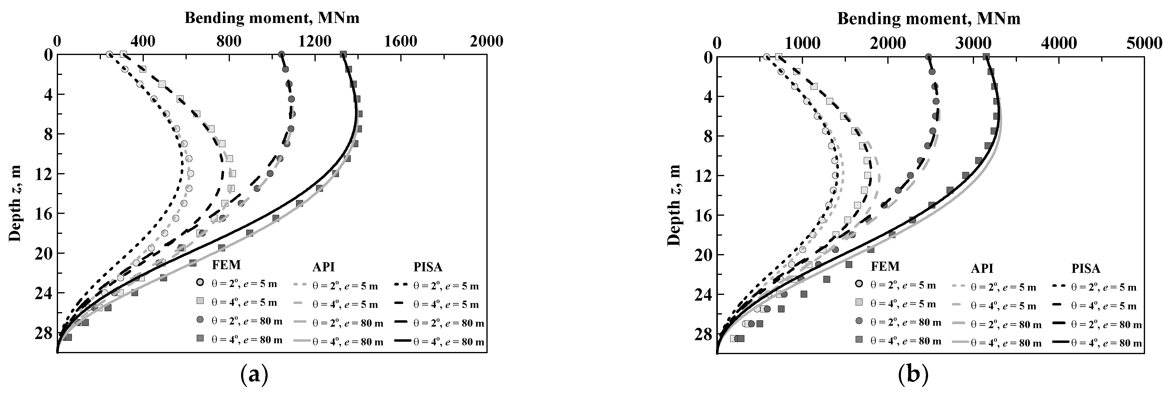
(e)
The bending moment profiles of the rigid monopiles are extremely insensitive to the p-y models. While the API and PISA p-y models are defined in completely different ways, the predicted bending moment profiles are almost equal and comparable to the three-dimensional FE simulation results.
(f)
The mobilized soil resistance increases with depth at shallow zone and then decreases to zero at rotation center for all the monopiles. This is attributed to the unique failure mechanism of rigid monopiles. A wedge failure at shallow 0.4L depth and a plane rotational failure around rotation center at around 0.75L were observed.
(g)
The soil resistance coefficient K = P⁄(Dσv′) is independent of pile diameter and aspect ratio. However, its distribution and magnitude along the monopile are affected by the failure mechanism and density of sand, respectively. Although the influence of pile diameter and aspect ratio are correctly considered in the PISA model, the influence of failure mechanism is not included in the model.
It was found that the simplified pile–soil interaction model by assuming a linear distribution of soil resistance along the pile can well capture the lateral response of rigid monopiles under lateral loading. A normalization method was proposed and validated against the three-dimensional simulation results. Explicit formulation was provided for sands with different relative densities to allow a quick calculation of the combined bearing capacity of monopiles under different rotations.

Author Contributions

H.W., methodology, investigation, writing—original draft preparation; L.W., conceptualization, methodology, supervision, funding acquisition, writing—review and editing; Y.H., writing—review and editing; A.A., writing—review and editing; B.H., writing—review and editing; H.P., writing—review and editing. All authors have read and agreed to the published version of the manuscript.

Funding

The authors would like to acknowledge the supports from the financial supports provided by 2018YFE0109500), National Natural Science Foundation of China (51779221, 51909249 and 51939010) and Zhejiang Provincial Natural Science Foundation (LHZ20E090001, LQ19E090001).

Institutional Review Board Statement

Not applicable.

Informed Consent Statement

Not applicable.

Data Availability Statement

The data presented in this study are available on request.

Acknowledgments

The authors would like to thank the reviewers for their valuable comments.

Conflicts of Interest

The authors declare no conflict of interest.

References

  1. IEA. Renewables 2020, IEA, Paris. Available online: https://www.iea.org/reports/renewables-2020 (accessed on 1 May 2020).
  2. Ramírez, L.; Fraile, D.; Brindley, G. Offshore Wind in Europe: Key Trends and Statistics 2019; Wind Europe: Brussels, Belgium, 2020. [Google Scholar]
  3. Doherty, P.; Gavin, K. Laterally loaded monopile design for offshore wind farms. Proc. Inst. Civ. Eng. Energy 2012, 165, 7–17. [Google Scholar] [CrossRef] [Green Version]
  4. Li, Q.; Askarinejad, A.; Gavin, K. The impact of scour on the lateral resistance of wind turbine monopiles: An experimental study. Can. Geotech. J. 2020. [Google Scholar] [CrossRef]
  5. Li, Q.; Prendergast, L.J.; Askarinejad, A.; Chortis, G.; Gavin, K. Centrifuge Modeling of the Impact of Local and Global Scour Erosion on the Monotonic Lateral Response of a Monopile in Sand. Geotech. Test. J. 2020, 43, 1084–1100. [Google Scholar] [CrossRef]
  6. Cheng, X.; Diambra, A.; Ibraim, E.; Liu, H.; Pisanò, F. 3D FE-Informed Laboratory Soil Testing for the Design of Offshore Wind Turbine Monopiles. J. Mar. Sci. Eng. 2021, 9, 101. [Google Scholar] [CrossRef]
  7. Wang, H.; Bransby, M.F.; Lehane, B.M.; Wang, L.Z.; Hong, Y. Numerical investigation of the lateral behaviour of large diameter rigid piles in medium dense uniform sand. Géotechnique 2021. under review. [Google Scholar]
  8. Wang, H.; Lehane, B.M.; Bransby, M.F.; Wang, L.Z.; Hong, Y. Field and numerical study of the lateral response of rigid piles in sand. Acta Geotech. 2021. under review. [Google Scholar]
  9. Richards, I.A.; Bransby, M.F.; Byrne, B.W.; Gaudin, C.; Houlsby, G.T. Effect of Stress Level on Response of Model Monopile to Cyclic Lateral Loading in Sand. J. Geotech. Geoenviron. Eng. 2021, 147, 04021002. [Google Scholar] [CrossRef]
  10. McAdam, R.A.; Byrne, B.W.; Houlsby, G.T.; Beuckelaers, W.J.; Burd, H.J.; Gavin, K.G.; Lgoe, D.J.P.; Jardine, R.J.; Martin, C.M.; Wood, A.M.; et al. Monotonic laterally loaded pile testing in a dense marine sand at Dunkirk. Géotechnique 2020, 70, 986–998. [Google Scholar] [CrossRef]
  11. Reese, L.C.; Cox, W.R.; Koop, F.D. Analysis of laterally loaded piles in sand. In Proceedings of the 5th Annual Offshore Technology Conference, Houston, TX, USA, 5–7 May 1974; Volume II, pp. 473–485. Available online: https://onepetro.org/OTCONF/proceedings-abstract/74OTC/All-74OTC/OTC-2080-MS/110527 (accessed on 1 June 2021).
  12. Bogard, D.; Matlock, H. Simplified Calculation of p-y Curves for Laterally Loaded Piles in Sand; Earth Technology Corp: Longmont, CO, USA, 1980. [Google Scholar]
  13. O’Neill, M.W.; Murchison, J.M. An Evaluation of p-y Relationships in Sands; A Report to the American Petroleum Institute; University of Houston: Houston, TX, USA, 1983. [Google Scholar]
  14. Georgiadis, M.; Anagnostopoulos, C.; Saflekou, S. Centrifugal testing of laterally loaded piles in sand. Can. Geotech. J. 1992, 29, 208–216. [Google Scholar] [CrossRef]
  15. Kirkwood, P.B. Cyclic Lateral Loading of Monopile Foundations in Sand. Ph.D. Thesis, University of Cambridge, Cambridge, UK, 2016. [Google Scholar]
  16. Klinkvort, R.T. Centrifuge Modelling of Drained Lateral Pile-Soil Response: Application for Offshore Wind Turbine Support Structures. Ph.D. Thesis, Technical University of Denmark, Kongens Lyngby, Denmark, 2013. [Google Scholar]
  17. Zhu, B.; Li, T.; Xiong, G.; Liu, J.C. Centrifuge model tests on laterally loaded piles in sand. Int. J. Phys. Model. Géotechnique 2016, 16, 160–172. [Google Scholar] [CrossRef]
  18. Wang, H.; Wang, L.Z.; Hong, Y.; He, B.; Zhu, R.H. Quantifying the influence of pile diameter on the load transfer curves of laterally loaded monopile in sand. Appl. Ocean. Res. 2020, 101, 102196. [Google Scholar] [CrossRef]
  19. Suryasentana, S.K.; Lehane, B.M. Numerical derivation of CPT-based p-y curves for piles in sand. Géotechnique 2014, 64, 186–194. [Google Scholar] [CrossRef]
  20. Suryasentana, S.K.; Lehane, B.M. Updated CPT-based p-y formulation for laterally loaded piles in cohesion less soil under static loading. Géotechnique 2016, 66, 445–453. [Google Scholar] [CrossRef]
  21. API (American Petroleum Institute). Geotechnical and Foundation Design Considerations; API RP 2GEO; API: Washington, DC, USA, 2011. [Google Scholar]
  22. Lam, I.P.; Martin, G.R. Seismic Design of Highway Bridge Foundations. In Design Procedures and Guidelines, Vol. 2, Report No. FHWA/RD-86/102; U.S. Department of Transportation, Federal Highway Administration: Springfield, VI, USA, 1986. [Google Scholar]
  23. Ashour, M.; Helal, A. Contribution of Vertical Skin Friction to the Lateral Resistance of Large-Diameter Shafts. J. Bridg. Eng. 2014, 19, 289–302. [Google Scholar] [CrossRef]
  24. Byrne, B.W.; Mcadam, R.; Burd, H.J.; Houlsby, G.T.; Martin, C.M.; Zdravkovic, L.; Taborda DM, G.; Potts, D.M.; Jardine, R.J.; Sideri, M.; et al. New design methods for large diameter piles under lateral loading for offshore wind applications. In Proceedings of the 3rd International Symposium on Frontiers in Offshore Geotechnics—ISFOG, Oslo, Norway, 10–12 June 2015; pp. 705–710. [Google Scholar]
  25. Burd, H.J.; Taborda, D.M.; Zdravković, L.; Abadie, C.N.; Byrne, B.W.; Houlsby, G.T.; Gavin, K.G.; Igoe, D.J.P.; Jardine, R.J.; Martin, R.A.; et al. PISA design model for monopiles for offshore wind turbines: Application to a marine sand. Géotechnique 2020, 70, 1048–1066. [Google Scholar] [CrossRef] [Green Version]
  26. Achmus, M.; Abdel-Rahman, K.; Peralta, P. On the Design of Monopile Foundations with Respect to Static and Quasi-Static Cyclic Loading; European Wind Energy Association: Brussels, Belgium, 2005. [Google Scholar]
  27. Achmus, M.; Albiker, J.; Peralta, P.; Tom Wörden, F. Scale Effects in the Design of Large Diameter Monopiles; EWEA: Brussels, Belgium, 2011; pp. 326–328. [Google Scholar]
  28. Thieken, K.; Achmus, M.; Lemke, K. A new static p-y approach for piles with arbitrary dimensions in sand. Geotechnik 2015, 38, 267–288. [Google Scholar] [CrossRef]
  29. Ahmed, S.S.; Hawlader, B. Numerical Analysis of Large-Diameter Monopiles in Dense Sand Supporting Offshore Wind Turbines. Int. J. Géoméch. 2016, 16, 04016018. [Google Scholar] [CrossRef] [Green Version]
  30. Dassault Systèmes, ABAQUS 6.8 Analysis User’s Manual; Simulia Corp.: Providence, RI, USA, 2007; Available online: http://130.149.89.49:2080/v6.10/pdf_books/ANALYSIS_3.pdf (accessed on 1 June 2021).
  31. Achmus, M.; Kuo, Y.-S.; Abdel-Rahman, K. Behavior of monopile foundations under cyclic lateral load. Comput. Geotech. 2009, 36, 725–735. [Google Scholar] [CrossRef]
  32. Hong, Y.; Soomro, M.A.; Ng CW, W.; Wang, L.Z.; Yan, J.J.; Li, B. Tunneling under pile groups and rafts: Numerical parametric study on tension effects. Comput. Geotech. 2015, 68, 54–65. [Google Scholar] [CrossRef]
  33. Von Wolffersdorff, P.A. A hypoplastic relation for granular materials with a predefined limit state surface. Mech. Cohesive-Frict. Mater. Int. J. Exp. Model. Comput. Mater. Struct. 1996, 1, 251–271. [Google Scholar] [CrossRef]
  34. Niemunis, A.; Herle, I. Hypoplastic model for cohesionless soils with elastic strain range. Mech. Cohesive-Frict. Mater. 1997, 2, 279–299. [Google Scholar] [CrossRef]
  35. Kolymbas, D.I.H.D. An outline of hypoplasticity. Arch. Appl. Mech. 1991, 61, 143–151. [Google Scholar]
  36. Bauer, E. Calibration of a Comprehensive Hypoplastic Model for Granular Materials. Soils Found. 1996, 36, 13–26. [Google Scholar] [CrossRef] [Green Version]
  37. Gudehus, G. A Comprehensive Constitutive Equation for Granular Materials. Soils Found. 1996, 36, 1–12. [Google Scholar] [CrossRef] [Green Version]
  38. Wu, W.; Bauer, E. A simple hypoplastic constitutive model for sand. Int. J. Numer. Anal. Methods Geomech. 1994, 18, 833–862. [Google Scholar] [CrossRef]
  39. Herle, I.; Gudehus, G. Determination of parameters of a hypoplastic constitutive model from properties of grain assemblies. Mech. Cohesive-Frict. Mater. Int. J. Exp. Model. Comput. Mater. Struct. 1999, 4, 461–486. [Google Scholar] [CrossRef]
  40. Gudehus, G.; Amorosi, A.; Gens, A.; Herle, I.; Kolymbas, D.; Mašín, D.; Viggiani, G. The soilmodels. info project. Int. J. Numer. Anal. Methods Geomech. 2008, 32, 1571–1572. [Google Scholar] [CrossRef]
  41. Wang, H.; Wang, L.; Hong, Y.; Mašín, D.; Li, W.; He, B.; Pan, H. Centrifuge testing on monotonic and cyclic lateral behavior of large-diameter slender piles in sand. Ocean. Eng. 2021, 226, 108299. [Google Scholar] [CrossRef]
  42. Hong, Y.; Koo, C.H.; Zhou, C.; Ng, C.W.; Wang, L.Z. Small strain path-dependent stiffness of Toyoura sand: Laboratory measurement and numerical implementation. Int. J. Geomech. 2016, 17, 04016036. [Google Scholar] [CrossRef]
Figure 1. Typical p-y curves of API [21] and Burd et al. [25] at: (a) z = 2D, (b) z = 5 m.
Jmse 09 00618 g001
Figure 2. Normalized ultimate soil resistance profile against: (a) z/D, (b) z/L.
Jmse 09 00618 g002
Figure 3. Typical model mesh of monopile with diameter of 10 m under a loading height of 5 m.
Jmse 09 00618 g003
Figure 4. Comparison of measure and computed load-deflection response of centrifuge tests.
Jmse 09 00618 g004
Figure 5. Comparison of measure and computed bending moment profiles of centrifuge tests: (a) D = 4 m, (b) D = 6 m.
Jmse 09 00618 g005
Figure 6. Moment–rotation curves at the ground surface in 65% relative density sand: (a) D = 4 m, (b) D = 6 m, (c) D = 8 m, (d) D = 10 m.
Jmse 09 00618 g006
Figure 7. Pile deflection profiles under typical rotations and loading eccentricity in 65% relative density sand: (a) D = 4 m, (b) D = 10 m.
Jmse 09 00618 g007
Figure 8. Bending moment profiles under typical rotations and loading eccentricity in 65% relative density sand: (a) D = 4 m, (b) D = 10 m.
Jmse 09 00618 g008
Figure 9. Soil resistance profiles under typical rotations and loading eccentricity in 65% relative density sand: (a) D = 4 m, (b) D = 10 m.
Jmse 09 00618 g009
Figure 10. Soil resistance coefficient profiles at 4 degrees and under loading eccentricity in 65% relative density sand against: (a) z/D, (b) z/L.
Jmse 09 00618 g010
Figure 11. Displacement contour of different diameter and aspect ratio monopiles under the same pile deflection in 65% relative density sand.
Jmse 09 00618 g011
Figure 12. Force–moment diagram of monopiles in 65% relative density under different deflection criteria: (a) 10%D, (b) 2°, (c) 4°, (d) ultimate.
Jmse 09 00618 g012
Figure 13. Simplified pile–soil interaction mechanism.
Jmse 09 00618 g013
Figure 14. Normalized force–moment diagram of monopiles in 65% relative density sand under different deflection criteria.
Jmse 09 00618 g014
Figure 15. Moment–rotation curves at the ground surface in 40% relative density sand: (a) D = 4 m, (b) D = 6 m, (c) D = 8 m, (d) D = 10 m.
Jmse 09 00618 g015
Figure 16. Moment–rotation curves at the ground surface in 80% relative density sand: (a) D = 4 m, (b) D = 6 m, (c) D = 8 m, (d) D = 10 m.
Jmse 09 00618 g016aJmse 09 00618 g016b
Figure 17. Deflection and bending moment profiles in 40% and 80% relative density sands under a loading eccentricity of 5 m: (a) deflection profile, (b) bending moment profile.
Jmse 09 00618 g017
Figure 18. Soil resistance profiles in 40% and 80% relative density sands under a loading eccentricity of 5 m.
Jmse 09 00618 g018
Figure 19. Soil resistance coefficient profiles at 4 degrees in 40% and 80% relative density sands against: (a) z/D, (b) z/L.
Jmse 09 00618 g019
Figure 20. Mobilized friction angle contour of typical 10 m monopiles in loose, medium dense and dense sand at a pile rotation of 4 degrees.
Jmse 09 00618 g020
Figure 21. Normalized force–moment diagram of monopiles in 40% and 80% relative density sands under different deflection criteria: (a) Dr = 40%, (b) Dr = 80%. (Note: The dashed lines represent the capacity calculated based on the simplified mechanism in Figure 13 by assuming a constant K).
Jmse 09 00618 g021
Figure 22. Soil resistance coefficient K of sands with different relative densities for different deflection criteria.
Jmse 09 00618 g022
Table 1. The p-y models in API [21] and Burd et al. [25].
p-y ModelBackbone FormulationModel Parameter
API [21] p = A p u t a n h [ k z A p u y ] k = ( 0.008085 φ 2.45 26.09 ) × 10 3
p u =   min { ( C 1 z + C 2 D ) γ z C 3 D γ z
C 1 = 0.115 × 10 0.0405 φ
C 2 = 0.571 × 10 0.022 φ
C 3 = 0.646 × 10 0.0555 φ
A = 3 0.8 z D 0.9 for static
A = 0.9 for cyclic
Burd et al. [25] p ¯ = { p u ¯ 2 c b + b 2 4 a c   y ¯ y u ¯ p u ¯                   y ¯ y u ¯ y u ¯ = 146.1 92.11 D r
k = k 1 + k 2 z D
a = 1 2 n k 1 = 8.731 0.6982 D r
b = 2 n y ¯ y u ¯ ( 1 n ) ( p ¯ p u ¯ y ¯ k p u ¯ ) k 2 = 0.9178
n = 0.917 + 0.06193 D r
c = ( 1 n ) y ¯ k p u ¯ n y ¯ 2 y ¯ u 2 p u ¯ = p u ¯ 1 + p u ¯ 2 z L
p ¯ = p / ( σ v D ) p u ¯ 1 = 0.3667 + 25.89 D r
y ¯ = y G 0 / ( σ v D ) p u ¯ 2 = 0.3375 8.900 D r
Note: D is pile diameter, L is pile embedded length, z is depth, γ′ is effective soil weight, φ is soil friction angle, Dr is soil relative density, G0 is shear modulus, σv′ is vertical effective stress.
Table 2. Numerical simulation program.
ObjectiveRelative Density, DrDiameter, DEmbedded Length, LLoading Height, e
Model validation with centrifuge tests65%4 m60 m10 m
65%6 m60 m10 m
Numerical parametric study40%4–10 m30 m5–100 m
65%4–10 m30 m5–100 m
80%4–10 m30 m5–100 m
Table 3. Calibrated parameters of hypoplastic model for Toyoura sand [42].
DescriptionValues
Basic hypoplastic model [37]Effective angle of shearing resistance at critical state, φ c 31
Hardness of granulates (kPa), h s 2.6 × 10 6
Exponent in the power law for proportional compression, n 0.27
Minimum void ratio at zero pressure, e d 0 0.61
Maximum void ratio at zero pressure, e i 0 0.98
Critical void ratio at zero pressure, e c 0 1.1
Exponent, α 0.11
Exponent, β 4
Intergranular strain concept [29]Parameter controlling initial shear modulus upon 180° strain path reversal, m R 8
Parameter controlling initial shear modulus upon 90° strain path reversal, m T 4
Size of elastic range, R 2 × 10 5
Parameter controlling degradation rate of stiffness with strain, β r 0.15
Parameter controlling degradation rate of stiffness with strain, χ 1.0
Publisher’s Note: MDPI stays neutral with regard to jurisdictional claims in published maps and institutional affiliations.

