A Eulerian–Lagrangian Coupled Method for the Simulation of Submerged Granular Column Collapse

Abstract

A two-fluid Eulerian–Lagrangian coupled model is developed to investigate the complex interactions between solid particles and the ambient water during the process of submerged granular column collapse. In this model, the water phase is considered to be a Newtonian fluid, whereas the granular column is modeled as an elastic–perfectly plastic material. The water flow field is calculated by the mesh-based Eulerian Finite Volume Method (FVM), with the free surface captured by the Volume-of-Fluid (VOF) technique. The large deformation of the granular material is simulated by the mesh-free, particle-based Lagrangian Smoothed Particle Hydrodynamics method (SPH). Information transfer between Eulerian nodes and Lagrangian particles is performed by the aid of the SPH interpolation function. Both dry and submerged granular column collapses are simulated with the proposed model. Experiments of the submerged cases are also conducted for comparison. Effects of dilatancy (compaction) of initially dense (loose) packing granular columns on the mixture dynamics are investigated to reveal the mechanisms of different flow regimes. Pore water pressure field and granular velocity field are in good agreement between our numerical results and experimental observations, which demonstrates the capability of the proposed Eulerian–Lagrangian coupled method in dealing with complex submerged water–granular mixture flows.

1. Introduction

Submerged granular column collapse is a typical water–grain interaction problem which serves as a model to investigate many underwater natural and hazardous processes, such as debris flows [1], landslides [2], submarine avalanches [3], etc. A large amount of granular material (mud, sand, gravel or rocks) that starts flowing underwater can create a tsunami [4] and damage undersea cables, pipelines, etc. A most recent example is the 2018 Sunda Strait tsunami. On 22 December 2018, a tsunami devastated several coastal regions of Sumatra and Java, Indonesia. Hundreds of people are reported dead with thousands injured. The tsunami is believed to have been caused by the collapse of Anak Krakatau that followed an eruption of the Anak Krakatau volcano in the Sunda Strait. Due to its harmful impacts to the coastal regions and underwater structures, submerged granular column collapse has long been a research concern for geophysicists, hydrologists and underwater engineers.

Ref. [5] developed a depth-averaged version of two-phase flow equations to describe the initiation of underwater granular avalanches. The rheology of the granular phase is based on a shear-rate-dependent critical state theory and a rheological model proposed for immersed granular flows. Using these phenomenological constitutive equations, the model can describe both the dilatancy effects experienced by the granular skeleton during the initial deformation and the rheology of wet granular media when the flow is fully developed.

Ref. [6] derived a set of two-phase continuum equations for studying a compressible granular flow composed of homogenous solid particles and a Newtonian ambient fluid. They found that the hydrodynamic fluid pressure helps the solids transit from dense-compacted to dense-suspended granular flow, whereas the drag forces counteract the solids movement, especially within the near-wall viscous layer. Ref. [7] studied the dynamics of a dense granular flow composed of a binary mixture of small and large grains immersed in an ambient fluid. Segregation of small and large grains with the presence of ambient water was investigated.

Ref. [8] conducted the experimental research of the collapse of a granular column in a viscous liquid. The role of the initial volume fraction was investigated. They found that the morphology of the deposits is mainly controlled by the initial volume fraction of the granular mass and not by the aspect ratio of the column, an observation which differs from dry granular collapse. For initially loose packing columns, the collapse is over within the order of seconds, whereas for dense packing columns, the collapse could take as long as tens of seconds. Understanding how these complex media flow underwater remains a challenge.

Ref. [9] investigated the effect of an ambient fluid on the dynamics of collapse and spread of a granular column by means of the contact dynamics method and computational fluid dynamics. They found that the effects of fluid in viscous and fluid-inertial regimes are to both reduce the kinetic energy during collapse and enhance the flow by lubrication during spread. Hence, the runout distance of the granular material in a fluid may be below or equal to that in the absence of fluid due to compensation between these effects. They also found that for a given aspect ratio and packing fraction, the runout distance may be similar in the grain-inertial and fluid-inertial regimes but with considerably longer duration in the latter case.

Ref. [10] developed a mixture model to predict various flows involving high concentration liquid-particle mixtures. Compared with the experiments of Ref. [8], their approach gives reasonably good predictions for the case of initially loose columns, but it was unsuccessful in simulating the collapse of an initially dense columns. Ref. [11] also proposed a Eulerian–Eulerian two-phase model based on a collisional-frictional law for the granular stress to describe the underwater granular flows. However, free surface wave was not considered in their paper.

Recently, a two-fluid SPH mixture model to analyze the water-soil interactions was proposed by the authors [12,13,14,15]. With this mixture model, it is possible to investigate the temporal and spatial evolutions of the volume fractions of both constituents. Dilatancy or compaction of granular materials can also be taken into consideration in this model.

In this paper, a Eulerian–Lagrangian coupled method for the simulation of underwater granular column collapse is presented. There are some reasons for developing coupled methods. First, for the water phase, it often provides an environment for the granular flow. Using Lagrangian method to solve the environmental water flow problem is always difficult due to the time-consuming process of particle methods. In fact, large number of numerical particles are needed for the water phase and the interaction pair particles should be searched in a fast and efficient way. However, with a mesh-based method, the cell size can be much larger than the particle interval and the node connectivity remains fixed in most of the cases. Second, the water pressure term in the Lagrangian methods is difficult to calculate correctly due to the weak compressibility of the model. On the contrary, the mesh-based method can result in a very smoothed pressure field. Thus, the coupled method should be much more efficient and accurate than the particle methods, as illustrated by [16] where a novel methodology that combines the smoothed discrete particle hydrodynamics (SDPH) and the finite volume method (FVM) was developed to enhance the effective performance in solving the problems of gas-particle multiphase flows.

In this paper, the coupled framework of SDPH-FVM of [16] is extended to the water–granular mixture flow. For the water phase, FVM is employed to discretize the water flow field on a stationary grid to simulate the fluid motion. At the meanwhile, the SPH method is employed to simulate the large deformation of the granular phase. The proposed two-fluid mixture Eulerian–Lagrangian coupled model is applied to analyze the water–grain interactions during submerged granular column collapse. Experiments of the same scale are also conducted to verify the numerical results. Dilatancy or compaction effects of the granular materials on the formation of different regimes are analyzed, which helps reveal the mechanisms of granular material collapse in the presence of an ambient fluid.

This paper is organized as follows. In Section 2, the mathematical formulation of the mixture theory is given. Section 3 is devoted to the numerical implementation of the Eulerian–Lagrangian coupled method. Model validation and numerical simulation of underwater granular column collapse are presented in Section 4. Conclusions and remarks are given in Section 5.

2. Mathematical Formulation

2.1. Water-Soil Mixture Model

In the two-fluid mixture model, the grains and the fluid are described as two continuum phases characterized by individual velocities, stresses and interaction through hydrodynamic forces. For each phase we define partial densities ${\rho }_{\eta }$, partial velocities ${\mathit{v}}_{\eta }$, and partial stresses ${\mathit{\sigma }}_{\eta }$, with $\eta =l,s$ standing for fluid and solid, respectively. Each phase must satisfy individual balance laws for the conservation of mass

$$\begin{array}{c}\hfill \frac{{\mathrm{D}}^{\eta }{\rho }_{\eta }}{\mathrm{D}\mathrm{t}}=-{\rho }_{\eta }\nabla ·{\mathit{v}}_{\eta },\end{array}$$

(1)

and momentum

$$\begin{array}{c}\hfill \frac{\partial }{\partial t}\left({\rho }_{\eta }{\mathit{v}}_{\eta }\right)+\nabla ·({\rho }_{\eta }{\mathit{v}}_{\eta }\otimes {\mathit{v}}_{\eta })=\nabla ·{\mathit{\sigma }}_{\eta }+{\rho }_{\eta }\mathit{g}+{\mathit{f}}_{\eta },\end{array}$$

(2)

where ⊗ is the dyadic product, $\mathit{g}$ the gravitational acceleration, ${\mathrm{D}}^{\eta }(·)/\mathrm{D}t$ the material time derivative along the path of particles of $\eta$ phase with $\frac{D^{\eta }(·)}{Dt}=\frac{\partial (·)}{\partial t}+{\mathit{v}}_{\eta }·\nabla (·)$, ${\mathit{f}}_{\eta }$ the inter-phase force exerted on phase $\eta$ by the other constituent, satisfying the Newton’s third law, i.e., ${\mathit{f}}_l+{\mathit{f}}_s=0$. Making use of Equation (1), the momentum Equation (2) can be rewritten as

$$\begin{array}{c}\hfill {\rho }_{\eta }\frac{{\mathrm{D}}^{\eta }{\mathit{v}}_{\eta }}{\mathrm{D}\mathrm{t}}=\nabla ·{\mathit{\sigma }}_{\eta }+{\rho }_{\eta }\mathit{g}+{\mathit{f}}_{\eta }.\end{array}$$

(3)

The above governing Equations (1) and (3) are expressed with partial variables, but the constitutive relationships are written with intrinsic (or true) variables as if they were single-phase flows. Thus, it is necessary to postulate the relationship of both kinds of variables. Here it is assumed that

$$\begin{array}{c}\hfill {\rho }_{\eta }={\varphi }_{\eta }{\tilde{\rho }}_{\eta },{\mathit{v}}_{\eta }={\tilde{\mathit{v}}}_{\eta },\end{array}$$

(4)

where variables with a tilde ($\tilde{}$) denote intrinsic variables, and ${\varphi }_{\eta }$ is the volume fraction of phase $\eta$, satisfying the saturation condition of ${\varphi }_l+{\varphi }_s=1$.

For the stress, we assume that

$$\begin{array}{c}\hfill {\mathit{\sigma }}_s={\varphi }_s{\tilde{\mathit{\sigma }}}_s,{\mathit{\sigma }}_l=-p\mathit{I}+{\varphi }_l{\tilde{\mathit{\tau }}}_l,\end{array}$$

(5)

where ${\tilde{\mathit{\sigma }}}_s$ is the intrinsic stress of the granular material, p the pore water pressure, and ${\tilde{\mathit{\tau }}}_l$ the intrinsic deviatoric stress tensor of the water. The volume fractions ${\varphi }_s$ and ${\varphi }_f$ in (5) imply that stresses are only acted on part of each constituent due to the porosity of the granular material. The interaction force ${\mathit{f}}_s$ (i.e., $-{\mathit{f}}_l$) is assumed to be in the form

$$\begin{array}{c}\hfill {\mathit{f}}_s=-{\varphi }_s\nabla p+C_d({\mathit{v}}_l-{\mathit{v}}_s).\end{array}$$

(6)

Here the first term on the right-hand side can be identified as a buoyancy force and the second term is simply an inter-phase resistance term, with $C_d$ being the drag coefficient. $C_d$ can be calculated according to the Darcy’s law [13].

In this study, the water phase is calculated in the Eulerian framework, thus it is convenient to rewrite the momentum equations of water as

$$\begin{array}{c}\frac{\partial {\mathit{v}}_l}{\partial t}+{\mathit{v}}_l·\nabla {\mathit{v}}_l=-\frac{1}{{\tilde{\rho }}_l}\nabla p+\nu {\nabla }^2{\mathit{v}}_l+\frac{1}{{\rho }_l}{\tilde{\mathit{\tau }}}_l·\nabla {\varphi }_l+\mathit{g}-\frac{C_d}{{\rho }_l}({\mathit{v}}_l-{\mathit{v}}_s),\hfill \end{array}$$

(7)

where use has been made of

$$\begin{array}{ccc}& & \frac{1}{{\rho }_l}\nabla ·\left({\varphi }_l{\tilde{\mathit{\tau }}}_l\right)=\frac{{\varphi }_l}{{\rho }_l}\nabla ·{\tilde{\mathit{\tau }}}_l+\frac{1}{{\rho }_l}{\tilde{\mathit{\tau }}}_l·\nabla {\varphi }_l\hfill \\ & & =\frac{\mu }{{\tilde{\rho }}_l}\nabla ·{\widetilde{\mathit{ϵ}}}_l+\frac{\mu }{{\rho }_l}{\widetilde{\mathit{ϵ}}}_l·\nabla {\varphi }_l=\nu \nabla ·{\widetilde{\mathit{ϵ}}}_l+\frac{\mu }{{\rho }_l}{\widetilde{\mathit{ϵ}}}_l·\nabla {\varphi }_l.\hfill \end{array}$$

(8)

The shear stress tensor ${\tilde{\mathit{\tau }}}_l$ for water phase is given by

$$\begin{array}{c}\hfill {\tilde{\tau }}_l^{\alpha \beta }=\mu {\tilde{\epsilon }}_l^{\alpha \beta },\end{array}$$

(9)

where $\mu$ is the dynamic viscosity of the water, $\nu =\frac{\mu }{{\tilde{\rho }}_l}$ the kinematic viscosity, and the strain rate tensor ${\tilde{\epsilon }}_l^{\alpha \beta }$ is defined as

$$\begin{array}{c}\hfill {\tilde{\epsilon }}_l^{\alpha \beta }={\epsilon }_l^{\alpha \beta }=\frac{\partial {\mathit{v}}_l^{\beta }}{\partial x^{\alpha }}+\frac{\partial {\mathit{v}}_l^{\alpha }}{\partial x^{\beta }}-\frac{2}{3}\left(\frac{\partial {\mathit{v}}_l^{\gamma }}{\partial x^{\gamma }}\right){\delta }^{\alpha \beta },\end{array}$$

(10)

in which ${\delta }^{\alpha \beta }$ is the Kronecker delta symbol, and $\gamma$ is a dummy index applicable to Einstein’s summation convention.

The liquid phase is allowed to have limited compressibility, in which case Equation (1) for water can be written as

$$\begin{array}{c}\hfill \frac{1}{{\rho }_l{c}_l^2}\frac{\partial p}{\partial t}+\nabla ·{\mathit{v}}_l=0,\end{array}$$

(11)

where the constant $c_l$ is the speed of sound in the fluid. For incompressible fluids $1/c_l^2$ is set to zero. In the limited compressibility model density changes are assumed to be small (say less than $1\%$) and the ${\rho }_l$ appearing in the pressure gradient terms in Equation (11) can be treated as constant. An artificial sound speed in water is set to a value lower than the physical one to obtain a higher time step size according to the Courant number. The staggered grid method is employed to discretize the pressure and velocity fields. A weakly formulation of the continuous equation is applied to achieve the pressure iteratively.

A finite volume method (FVM) is used to solve the equations of water phase. Underwater granular column collapse can result in free surface waves which can be captured using the volume of fluid (VOF, Hirt and Nichols [17]) method. It is assumed that near the free surface the granular phase vanishes and there exists only the water and air phases separated by the free surface. The time dependence of the VOF function F, defined as the volume fraction of the water in a computational grid cell across the water-air interface, is governed by

$$\begin{array}{c}\hfill \frac{\partial F}{\partial t}+{\mathit{v}}_l·\nabla F=0.\end{array}$$

(12)

For an incompressible fluid, Equation (12) may be combined with Equation (1) to yield

$$\begin{array}{c}\hfill \frac{\partial F}{\partial t}+\nabla ·\left({\mathit{v}}_{l}F\right)=0.\end{array}$$

(13)

As we have seen, there are two volume fraction functions: the first one is the volume fraction F to distinguish the free surface between the water and the air; the second is the volume fraction ${\varphi }_l$ denoting the water content in the liquid-granular mixture. The first volume fraction is introduced by the VOF method. The second volume fraction is introduced by the mixture theory.

2.2. Constitutive Laws for the Solid Phase

Consider the granular material as an elastic–perfectly plastic material with a Drucker-Prager yield criterion

$$\begin{array}{c}\hfill Y(I_1,J_2)=\sqrt{J_2}+{\alpha }_{\theta }{I}_1-k_c,\end{array}$$

(14)

where $I_1$ is the first invariant of the total stress tensor ${\tilde{\sigma }}_s^{\alpha \beta }$, and $J_2$ is the second invariant of the deviatoric stress tensor ${\tilde{\tau }}_s^{\alpha \beta }$, defined by

$$\begin{array}{c}\hfill I_1={\tilde{\sigma }}_s^{xx}+{\tilde{\sigma }}_s^{yy}+{\tilde{\sigma }}_s^{zz},J_2=\frac{1}{2}{\tilde{\tau }}_s^{\alpha \beta }{\tilde{\tau }}_s^{\alpha \beta }.\end{array}$$

(15)

For plane strain problem, ${\alpha }_{\theta }$ and $k_c$ in Equation (14) are determined by (see Bui et al. [18])

$$\begin{array}{c}\hfill {\alpha }_{\theta }=\frac{tan\theta }{\sqrt{9+12{tan}^2\theta }},k_c=\frac{3c}{\sqrt{9+12{tan}^2\theta }},\end{array}$$

(16)

where c and $\theta$ are the cohesion and the friction angle of granular materials, respectively.

A plastic flow rule is needed to describe the development of the plastic deformation. The flow rule is characterized by the plastic potential function H. If H is chosen to be equal to the yield function Y, we then use the so-called associated flow rule, with which the constitutive relation can be written as [18]

$$\begin{array}{c}\hfill {\dot{\tilde{\sigma }}}_s^{\alpha \beta }-{\tilde{\sigma }}_s^{\alpha \gamma }{\dot{\omega }}_s^{\beta \gamma }-{\tilde{\sigma }}_s^{\gamma \beta }{\dot{\omega }}_s^{\alpha \gamma }=2G{\dot{e}}_s^{\alpha \beta }+K{\dot{\epsilon }}_s^{\gamma \gamma }{\delta }^{\alpha \beta }-\dot{\lambda }\left[3{\alpha }_{\theta }K{\delta }^{\alpha \beta }+G/\sqrt{J_2}{\tilde{\tau }}_s^{\alpha \beta }\right],\end{array}$$

(17)

where ${\dot{e}}_s^{\alpha \beta }$ is the deviatoric strain rate tensor ${\dot{\epsilon }}_s^{\alpha \beta }$, G the shear modulus, K the bulk modulus. Here the Jaumann rate has been applied, with the rotational rate tensor ${\dot{\omega }}_s^{\alpha \beta }$ defined as

$$\begin{array}{c}\hfill {\dot{\omega }}_s^{\alpha \beta }=\frac{1}{2}\left(\frac{\partial v_s^{\alpha }}{\partial x^{\beta }}-\frac{\partial v_s^{\beta }}{\partial x^{\alpha }}\right).\end{array}$$

(18)

The rate of change of plastic multiplier $\dot{\lambda }$ is calculated by

$$\begin{array}{c}\hfill \dot{\lambda }=\frac{3{\alpha }_{\theta }K{\dot{\epsilon }}_s^{\gamma \gamma }+(G/\sqrt{J_2}){\tilde{\tau }}_s^{\alpha \beta }{\dot{\epsilon }}_s^{\alpha \beta }}{9{\alpha }_{\theta }^{2}K+G}.\end{array}$$

(19)

The second type of flow rule is the non-associated flow rule, in which the plastic potential function H takes the form

$$\begin{array}{c}\hfill H=\sqrt{J_2}+3I_{1}sin\psi ,\end{array}$$

(20)

where $\psi$ is the dilatancy angle. In this case, the constitutive relation for the granular material is

$$\begin{array}{c}\hfill {\dot{\tilde{\sigma }}}_s^{\alpha \beta }-{\tilde{\sigma }}_s^{\alpha \gamma }{\dot{\omega }}_s^{\beta \gamma }-{\tilde{\sigma }}_s^{\gamma \beta }{\dot{\omega }}_s^{\alpha \gamma }=2G{\dot{e}}_s^{\alpha \beta }+K{\dot{\epsilon }}_s^{\gamma \gamma }{\delta }^{\alpha \beta }-\dot{\lambda }\left[9Ksin\psi {\delta }^{\alpha \beta }+G/\sqrt{J_2}{\tilde{\tau }}_s^{\alpha \beta }\right],\end{array}$$

(21)

where the rate of change of plastic multiplier $\dot{\lambda }$ is given as

$$\begin{array}{c}\hfill \dot{\lambda }=\frac{3{\alpha }_{\theta }K{\dot{\epsilon }}_s^{\gamma \gamma }+(G/\sqrt{J_2}){\tilde{\tau }}_s^{\alpha \beta }{\dot{\epsilon }}_s^{\alpha \beta }}{27{\alpha }_{\theta }Ksin\psi +G}.\end{array}$$

(22)

In this study, a critical state theory [5,19] is employed to determine the dilatancy angle $\psi$

$$\begin{array}{ccc}& & \frac{1}{{\varphi }_s}\frac{\mathrm{d}{\varphi }_s}{\mathrm{d}t}=-tan\psi \left|\dot{\gamma }\right|,\hfill \end{array}$$

(23)

$$\begin{array}{ccc}& & tan\psi =K_3({\varphi }_s-{\varphi }_{eq}),\hfill \end{array}$$

(24)

where ${\varphi }_{eq}$ is the granular volume fraction obtained in the steady regime, $K_3$ is a constant, $|\dot{\gamma }|$ is the magnitude of the shear rate tensor (${\dot{\gamma }}_{ij}=\frac{1}{2}(v_{i,j}+v_{j,i})-\frac{1}{3}{v}_{\alpha ,\alpha }{\delta }_{ij}$), defined by its second invariant, i.e., $|\dot{\gamma }|=\sqrt{1/2{\dot{\gamma }}_{ij}{\dot{\gamma }}_{ij}}$. Equation (23) can be derived from the mass conservation equation and the definitions of the dilatancy angle $\psi$ and the strain $\gamma$ [20]. It implies only that dilatancy can cause variation of porosity which in turn affects the pore pressure and efficient solid stress, as well as the inter-granular friction. Equation (24) is a closure relation, obtained by fitting the experimental measurements. In this study, $K_3$ is set to 4.09, according to Pailha and Pouliquen [5]. Because Equations (23) and (24) act as a feedback control law for ${\varphi }_s$, this phenomenon is known as “pore pressure feedback” [21,22] and will be shown in our numerical simulations later.

Dilatancy (or compaction) also contributes to the inter-particle friction due to the geometrical entanglement. To reflect this, the friction angle $\theta$ in (16) should be replaced by $\theta +\psi$, see [15].

3. Eulerian–Lagrangian Coupled Method

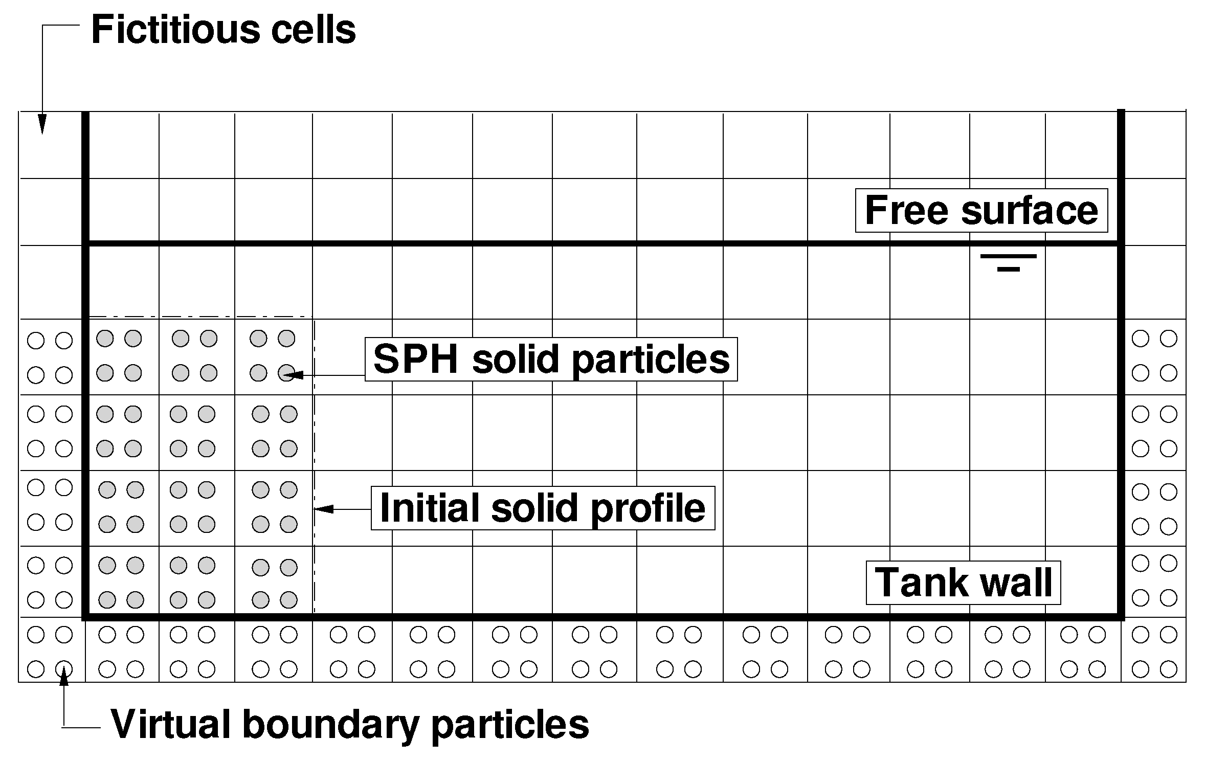
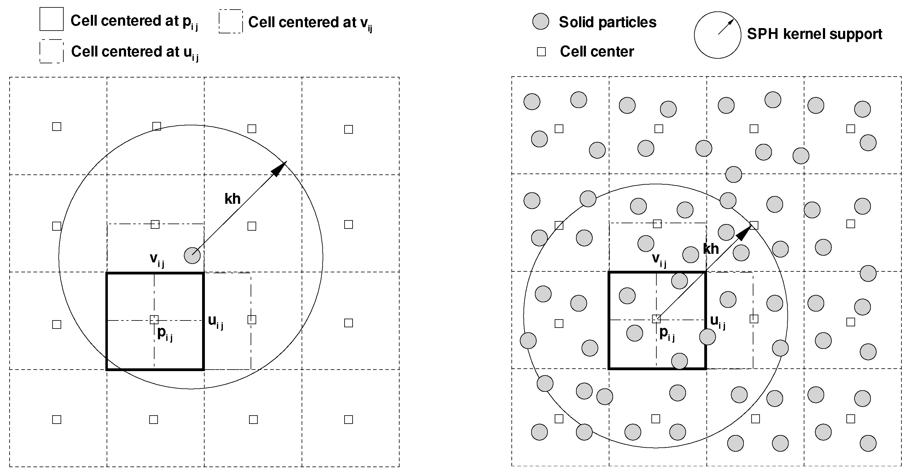
3.1. FVM and SPH Coupling

In the numerical simulation, the domain of water phase is discretized by Eulerian mesh, while the granular phase is discretized by material particles, as seen in Figure 1. Both fictitious cells and virtual boundary particles are used to implement the boundary conditions. The VOF code used is an adaptation of the SOLA-VOF code developed in the Los Alamos National Laboratory (Hirt and Nichols [17]). An in-house SPH code is developed to undertake the analysis of the granular phase, for the problem of submerged granular column collapse. In this section, the VOF and SPH implementations are not described in detail. Interested readers are referred to [17] for VOF method and [12,13] for SPH implementation.

The key issue is the transfer of the information between Eulerian grid nodes and Lagrangian particles. The interpolation process is depicted in Figure 2. In our approach, this transfer is accomplished using the smooth kernel of the SPH method. In fact, the foundation of SPH method is based on the following integral representation of a field function $f\left(\mathit{x}\right)$:

$$\begin{array}{c}\hfill \langle f\left(\mathit{x}\right)\rangle ={\int }_{\mathsf{\Omega }}f\left({\mathit{x}}^{\prime }\right)W(\mathit{x}-{\mathit{x}}^{\prime },h)\mathrm{d}{\mathit{x}}^{\prime },\end{array}$$

(25)

where $W(\mathit{x}-{\mathit{x}}^{\prime },h)$ is called the kernel or smoothing function, and h is the smoothing length which defines the influence domain $\mathsf{\Omega }$ of the kernel $W(\mathit{x}-{\mathit{x}}^{\prime },h)$. In SPH method, the computational domain is discretized into a finite number of particles. The continuous integral representation of the field variable $f\left(\mathit{x}\right)$ at position ${\mathit{x}}_i$, in Equation (25), is then approximated by summation over the neighboring particles in the support domain, as

$$\begin{array}{c}\hfill \langle f\left({\mathit{x}}_i\right)\rangle \approx \sum _{j=1}^N\frac{m_j}{{\rho }_j}f\left({\mathit{x}}_j\right)W_{ij},\end{array}$$

(26)

where $W_{ij}=W({\mathit{x}}_i-{\mathit{x}}_j,h)$; $m_j$ and ${\rho }_j$ are the mass and density of particle j at position ${\mathit{x}}_j$, respectively; N is the number of particles in the support domain of particle i. A Wendland quintic kernel function is chosen in this study to perform the SPH interpolation approximation (Wang et al. [12]).

SPH method suffers from the so-called boundary deficiency problem due to the truncation of the support domain of the kernel function $W_{ij}$ by the boundary. To overcome this deficiency, a re-normalization technique is introduced to perform the SPH approximation (Chen et al. [16]):

$$\begin{array}{c}\hfill \langle f\left({\mathit{x}}_i\right)\rangle \approx \frac{{\sum }_{j=1}^N\frac{m_j}{{\rho }_j}f\left({\mathit{x}}_j\right)W_{ij}}{{\sum }_{j=1}^N\frac{m_j}{{\rho }_j}{W}_{ij}},\end{array}$$

(27)

where N is the number of particles in the support domain of particle i. With this re-normalization technique, information transfer from the solid particles to the grid nodes can be implemented by

$$\begin{array}{c}\hfill \langle f\left({\mathit{x}}_g\right)\rangle \approx \frac{{\sum }_{i=1}^{N_p}\frac{m_i}{{\rho }_i}f\left({\mathit{x}}_i\right)W_{ig}}{{\sum }_{i=1}^{N_p}\frac{m_i}{{\rho }_i}{W}_{ig}},\end{array}$$

(28)

where ${\mathit{x}}_g$ is the node position, $N_p$ is the number of solid particles in the support domain of grid node ${\mathit{x}}_g$. Analogously, information transfer from the grid nodes to a certain particle can be done by

$$\begin{array}{c}\hfill \langle f\left({\mathit{x}}_i\right)\rangle \approx \frac{{\sum }_{g=1}^{N_g}\frac{m_g}{{\rho }_g}f\left({\mathit{x}}_g\right)W_{ig}}{{\sum }_{g=1}^{N_g}\frac{m_g}{{\rho }_g}{W}_{ig}},\end{array}$$

(29)

where $N_g$ is the number of grid nodes in the support domain of the solid particle at ${\mathit{x}}_i$; $m_g$ and ${\rho }_g$ are, in principle, the mass and density of the water particles at grid node ${\mathit{x}}_g$, respectively. However, due to the Eulerian nature of the FVM method for the water phase, no water particles exist in the present method. In fact, $m_g/{\rho }_g$ represents a volume of fluid at the position ${\mathit{x}}_g$, thus the volume of the cell centered at ${\mathit{x}}_g$ can be used as $m_g/{\rho }_g$ to perform the interpolation in (29). Usually, the cell size is larger than the particle interval. The support domain of the interpolation function should therefore be enlarged to contain sufficiently many grid nodes.

3.2. Special Treatment of the Pore Pressure

The interaction force ${\mathit{f}}_s$ in (6) contains the buoyancy force $-{\varphi }_s\nabla p$. Using the SPH approximation rule (26), this term for the solid particle i would be approximated by

$$\begin{array}{c}\hfill -{\varphi }_i\nabla p_i\approx -{\varphi }_i\sum _g^{N_g}\frac{m_g}{{\rho }_g}{p}_g{\nabla }_i{W}_{ig},\end{array}$$

(30)

where subscript g means the nearby grid nodes. However, this approximation results often in numerical instability (shown later). Thus, the buoyancy force $-{\varphi }_s\nabla p$ at solid particle i is replaced by

$$\begin{array}{c}\hfill -{\varphi }_i\nabla p_i\approx -{\varphi }_i\sum _g^{N_g}\frac{m_g}{{\rho }_g}(p_g-p_i^{\prime }){\nabla }_i{W}_{ig},\end{array}$$

(31)

where $p_i^{\prime }$ is the pore water pressure at the location of solid particle i, obtained using the re-normalized SPH interpolation approximation (29).

Water volume fraction ${\varphi }_g$ on a grid node ${\mathit{x}}_g$ is calculated, according to the saturation condition ${\varphi }_l+{\varphi }_s=1$, by

$$\begin{array}{c}\hfill {\varphi }_l\left({\mathit{x}}_g\right)=1-\frac{1}{{\tilde{\rho }}_s}\sum _i^{}{m}_i{W}_{gi},\end{array}$$

(32)

where the summation term gives solid volume fraction ${\varphi }_s$ at the position of grid node ${\mathit{x}}_g$.

3.3. Time Integration and Boundary Conditions

For the FVM simulation, a forward Eulerian integration scheme is employed to integrate Equations (7), (11) and (13) for the fluid phase, while for the SPH calculation, a second-order accurate numerical integration scheme, namely the Leap-Frog (LF) method is adopted here to integrate Equations (1), (3), (17) or (21), and (23) for the granular phase (see Wang et al. [14]). The time step size is controlled by the so-called Courant-Fredrich-Levy (CFL) condition and additional constraints due to the interaction forces and viscous diffusion

$$\begin{array}{c}\hfill \mathsf{\Delta }t\le 0.3min(h/c_l,h/c_s),\mathsf{\Delta }t\le 0.2min(h/f_l,h/f_s),\mathsf{\Delta }t\le 0.2min(h^2/\nu ),\end{array}$$

(33)

where $\mathsf{\Delta }t$ is the time step size; h is the smoothing length of particles; $c_l$ and $c_s$ are the sound speed of water and grains, respectively; $f_l$ and $f_s$ are the drag forces acting on water particles and solid particles, respectively; $\nu$ is the water viscosity. The time step $\mathsf{\Delta }t$ for a simulation should be chosen to be the minimum value of the above constraints. Although Leap-Frog integration is a second-order method, in contrast to Eulerian integration scheme, which is only first order, the accuracy of the time stepping scheme of the coupled method is only first order.

In FVM simulation, in addition to the free surface boundary conditions treated by the VOF technique, it is necessary to set conditions at all mesh boundaries. At the mesh boundaries, a variety of conditions may be set using layers of fictitious cells surrounding the mesh. The basic idea is to set values for the dependent variables in the fictitious cells such that the desired boundary conditions are met at the boundaries, see [17]. For the SPH simulation, the wall boundary is treated by the dynamic particle method, proposed by [23].

4. Simulations and Results Analysis

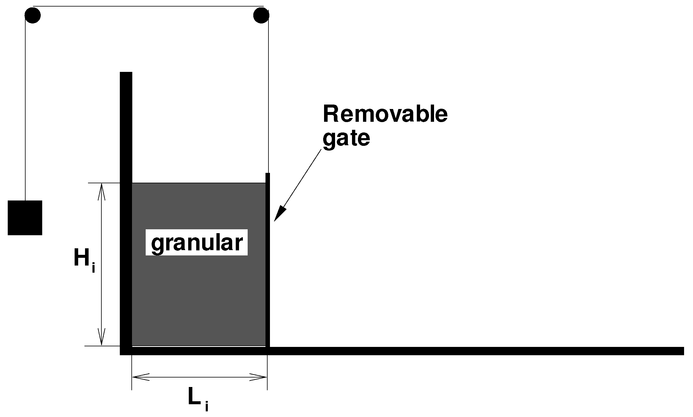
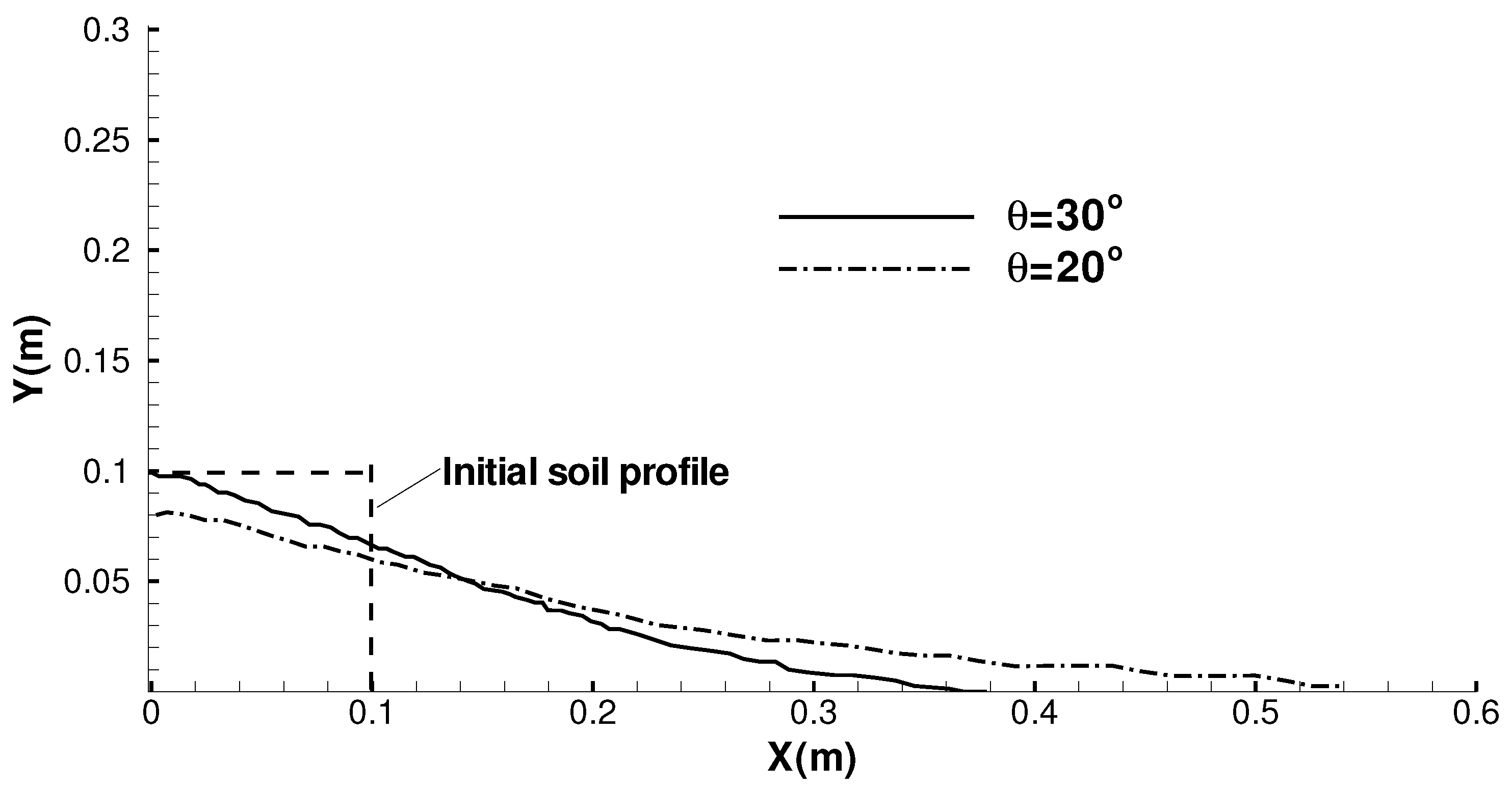
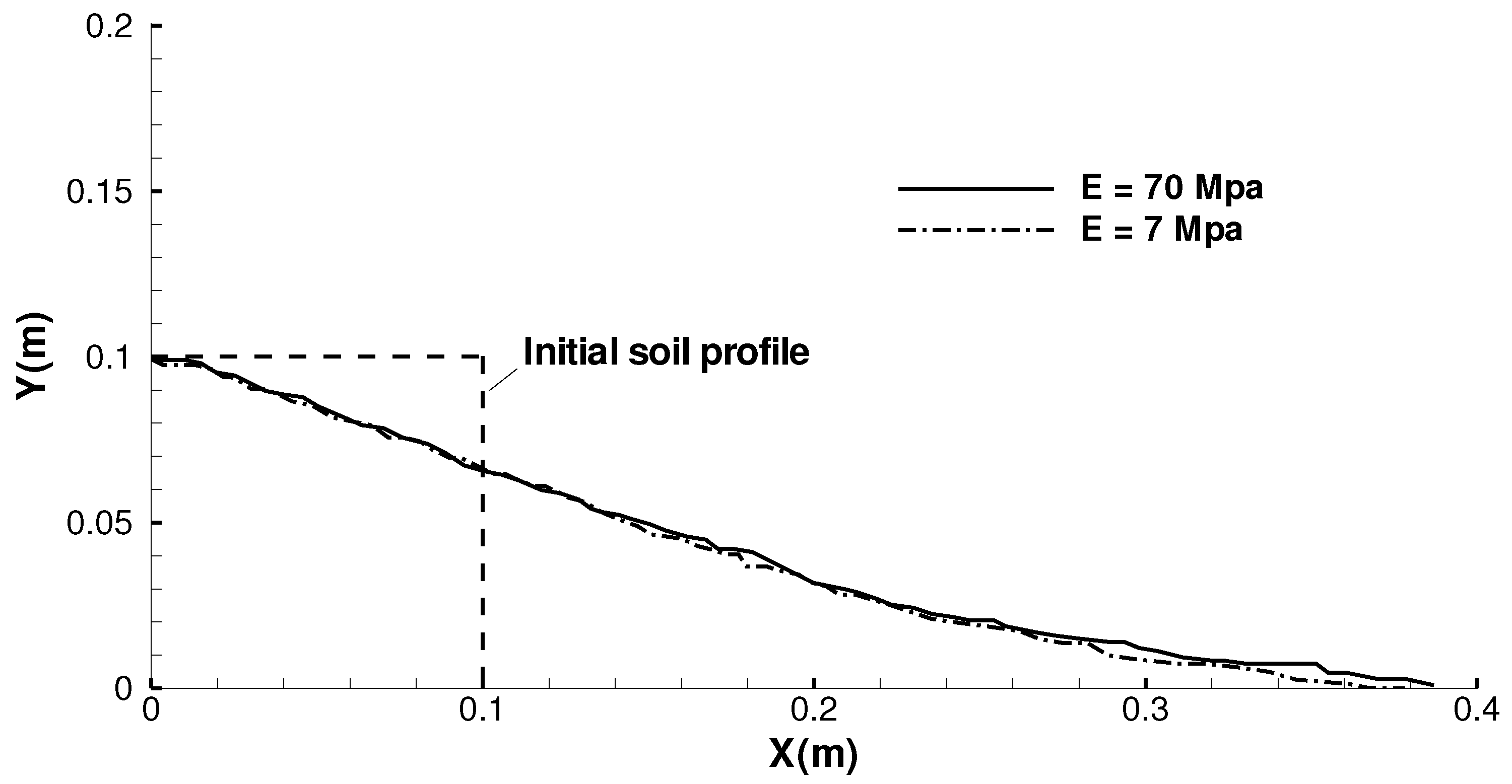
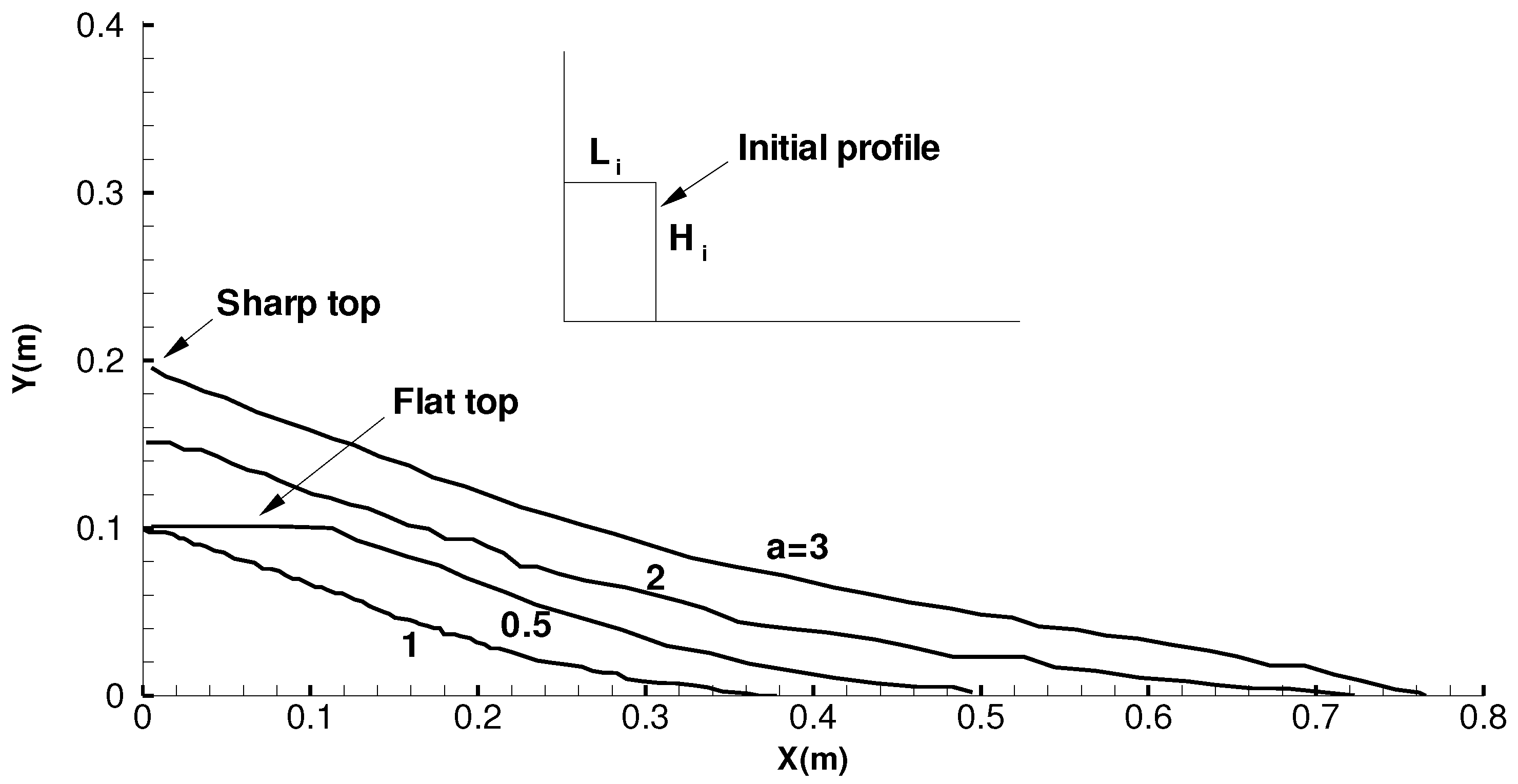
4.1. Dry Granular Column Collapse

We first apply the proposed SPH model to the problem of single-phase dry granular column collapse in the air. This problem has been studied by the present authors [12], using SPH method. In [12], we compared our numerical results with experimental and computational results of [18]. An excellent agreement was observed. Thus, in this section, only the effects of some material and geometrical parameters, such as the internal friction angle $\theta$, the material stiffness E and the aspect ratio a of the column, on the granular column collapse, are investigated.

We first investigate the case that a 2D granular column of 0.1 m wide and 0.1 m high is released at $t=0$. The initial configuration of the granular column is shown in Figure 3. Material properties for the granular medium are listed in

Table 1. Properties of the granular material used in the computation for an initially 10 cm × 10 cm ($L_i\times H_i$) dry granular column collapse in air.

Property	Symbol	Value
True density	${\tilde{\rho }}_s$	2700 $\mathrm{kg}/{\mathrm{m}}^3$
Young’s modulus	E	70 MPa
Poisson’s ration	$\nu$	0.3
Internal friction angle	$\theta$	${20}^{\circ }$
Cohesion	c	0
Dilatancy angle	$\psi$	$2.5^{\circ }$

. The granular material is assumed to be cohesionless. In the simulation, a total of 12,800 solid particles are used, with an initial particle spacing of 0.00125 m. The sound speed is chosen $c_s=150$ m/s, which is needed to control the time step size according to the CFL condition (33). The time step size is set to $\mathsf{\Delta }t=5\times {10}^{-6}$ s.

In this study, computations of the plastic behavior are based on the non-associated flow rule which results in the phenomenon of dilatancy. For the non-associated flow rule, the significance of dilatancy can be characterized by the dilatancy angle $\psi$. In the simulation for the dry granular collapse, the dilatancy angle $\psi$ is set to be constant, while for submerged cases, this variable is a dynamic quantity computed from the mixture rheology relationships (23) and (24), as seen in the next section, i.e., although in the dry case, a granular medium obeys a relaxation towards the critical state, we do not use the same dilatancy law as used in the submerged section with the dilatancy angle coupled with the volume fraction. We point out that although dilatancy can adjust the friction coefficient to some extends, its effect on the collapse dynamics of a granular medium is prominent only if it is interactive with the pore pressure feedback mechanism. Here for the dry case, a dilatancy angle $\psi ={2.5}^{\circ }$ is taken, which normally results in a relatively high dilatancy.

Figure 4 shows the influence of the internal friction angle $\theta$ on the morphology of the deposit, where two friction angles, namely ${\theta }_1={20}^{\circ }$ and ${\theta }_2={30}^{\circ }$, are considered, respectively. We can see that the runout distance of the granular column decreases with the increase of the internal friction angle. This is reasonable if we bear in mind the fact that the internal friction increases the strength of the granular material, as seen in Equation (14).

Figure 5 investigates the influence of the Young’s modulus E on the morphology of the deposit. Two values of E, i.e., 70 MPa and 7 MPa, are investigated. It can be seen that for dry granular column collapse, the morphology of the deposit is not sensitive to the Young’s modulus E of the granular material. Thus, in the following study, a typical value for the granular materials is used, namely $E=70$ MPa.

The influence of the aspect ratio a of the column on the morphology of the deposit is shown in Figure 6. The aspect ratio a is defined as $a=H_i/L_i$, where $H_i$ and $L_i$ denote the initial height and width of the granular column, respectively. We can see that for a granular column with high aspect ratio, say $a>1.0$ for example, the height of the deposit is lower than the initial height of the column, and at the end of the collapse, a pile with a sharp top is developed. However, in the case of low aspect ratio, $a<1.0$, the height of the column is almost unchanged during the collapse, leading to a pile of flat top at the end of the collapse. This result agrees with the experimental observations conducted by [24].

Ref. [18] pointed out that the use of the continuity Equation (1) in the current SPH application to dry granular material is optional and can be removed from the governing equations if the bulk density is kept constant. Retaining the continuity equation with the assumption of constant density corresponds to resolving the variation of void ratio or porosity of a granular material. The idea is illustrated in Figure 7, where numerical simulations with and without continuity Equation (1) are presented. We can see that the numerical results in these two cases are nearly the same, thus the continuity Equation (1) is not important for the simulation of dry soil column collapse. However, in the case of submerged granular column collapse, the continuity equation should be employed to resolve the variation of volume fraction of granular material, as seen in the next section.

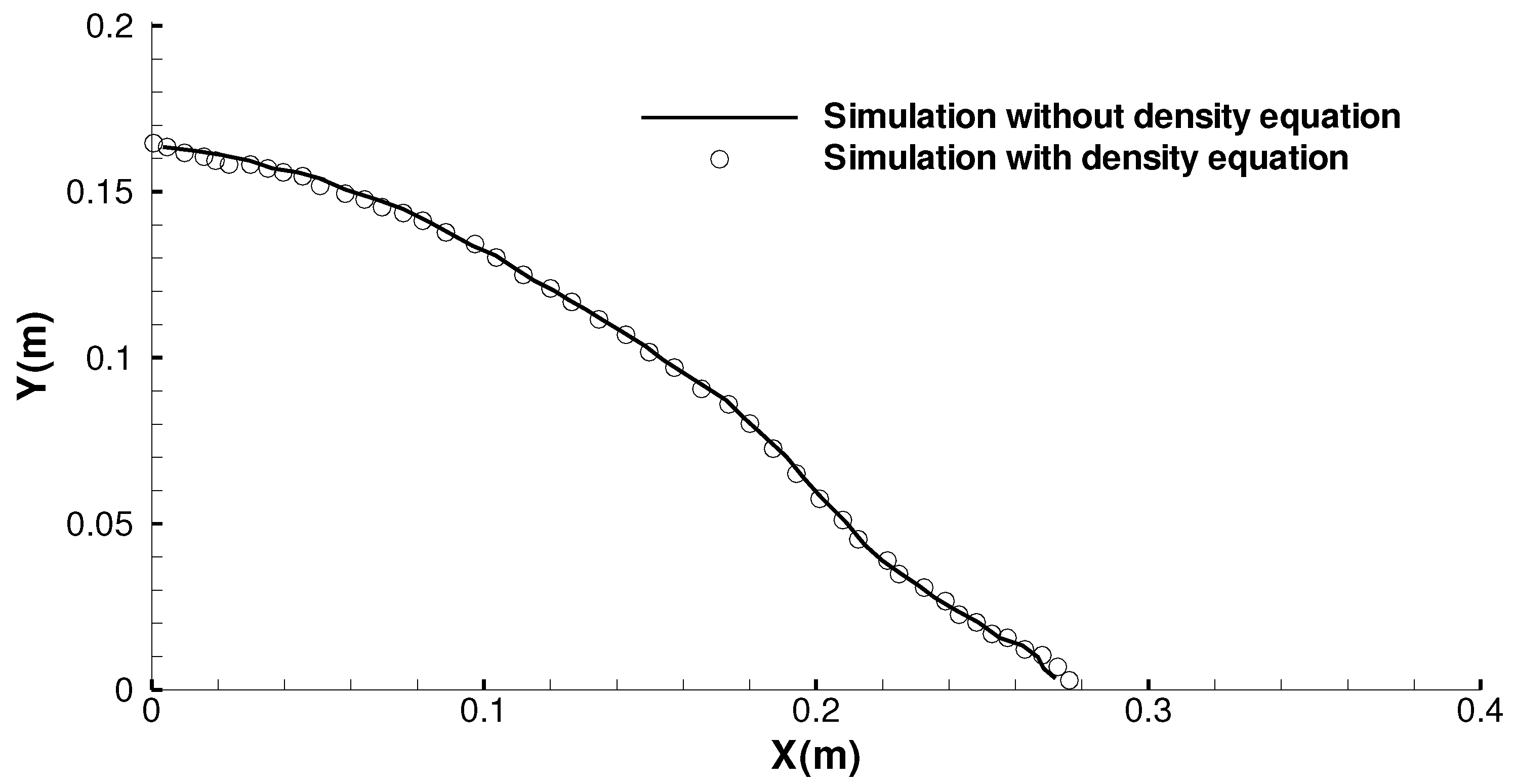
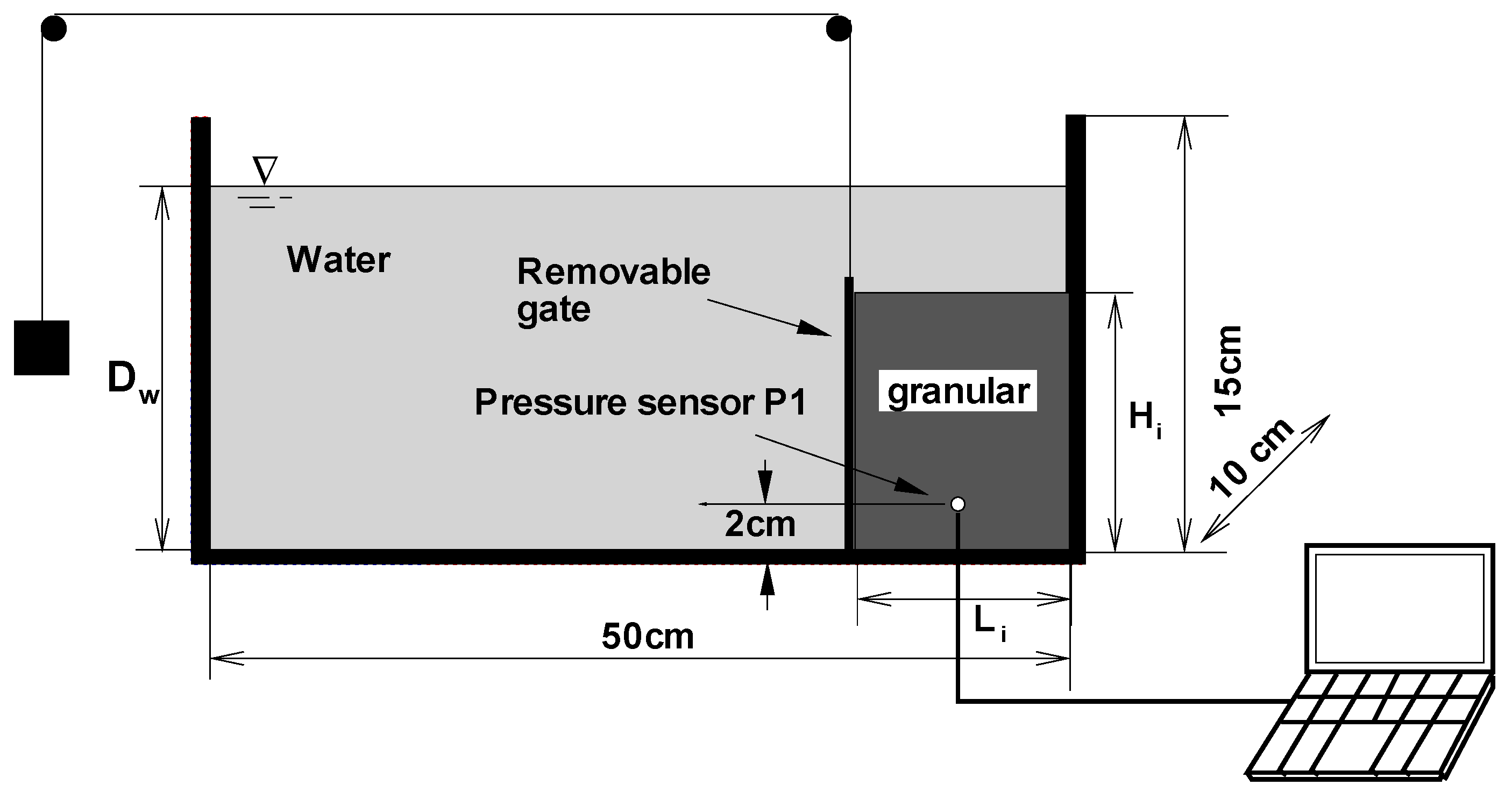
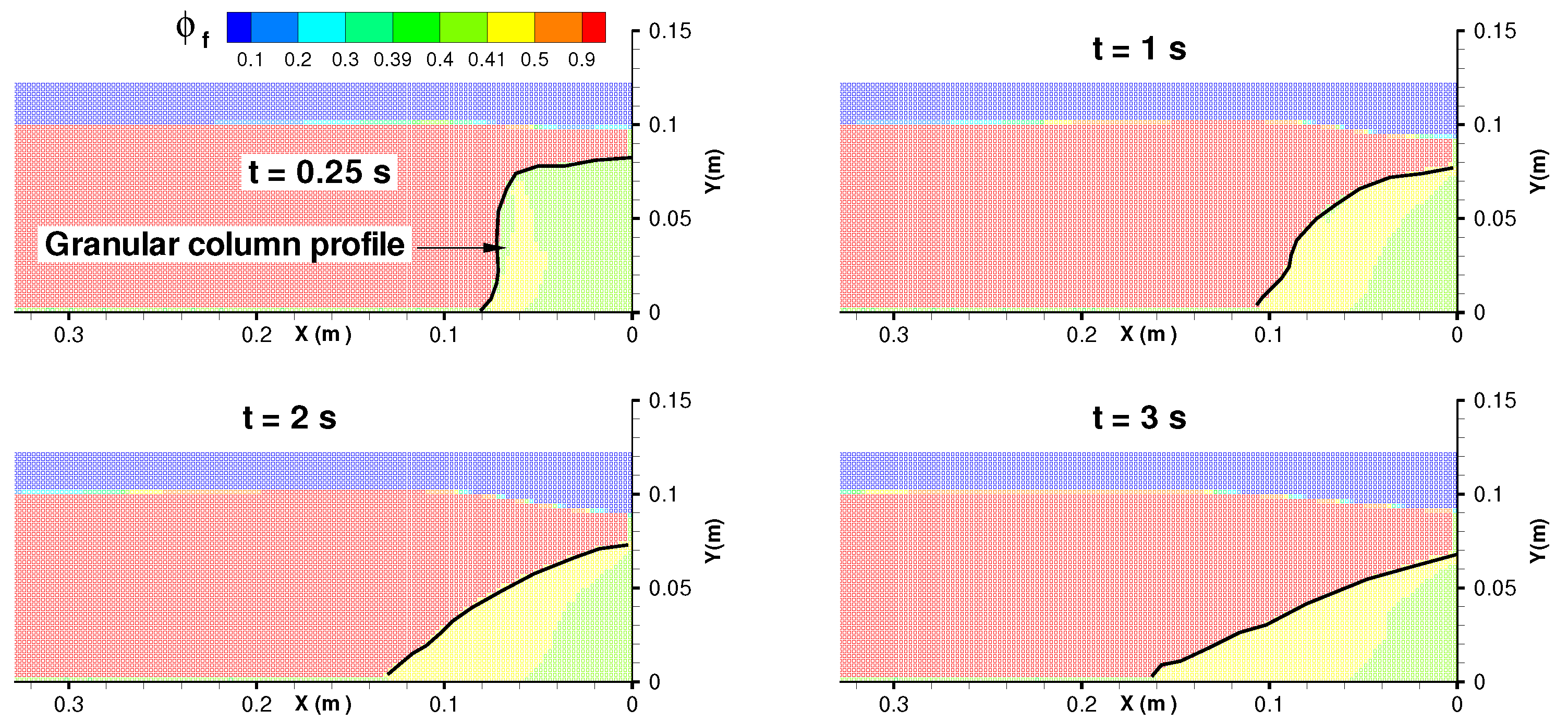
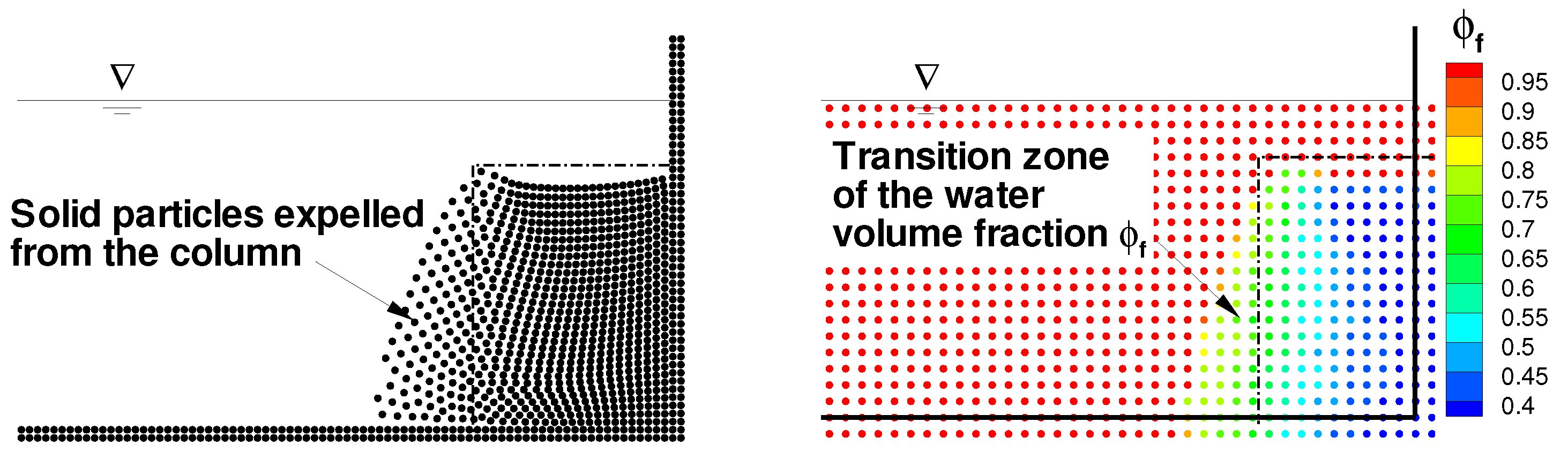
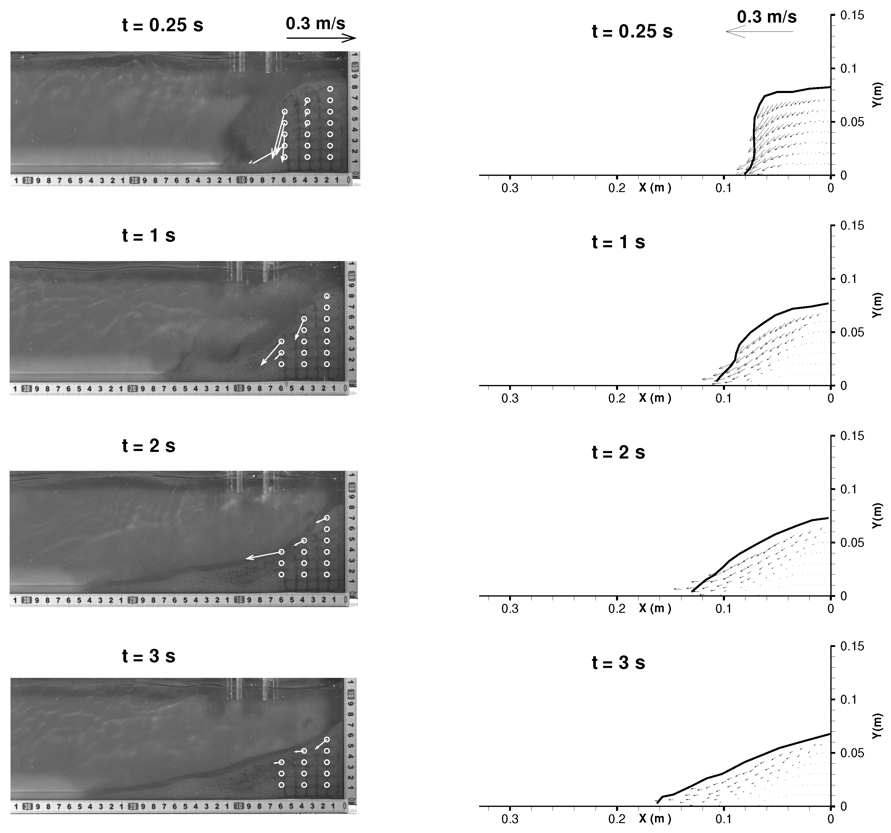
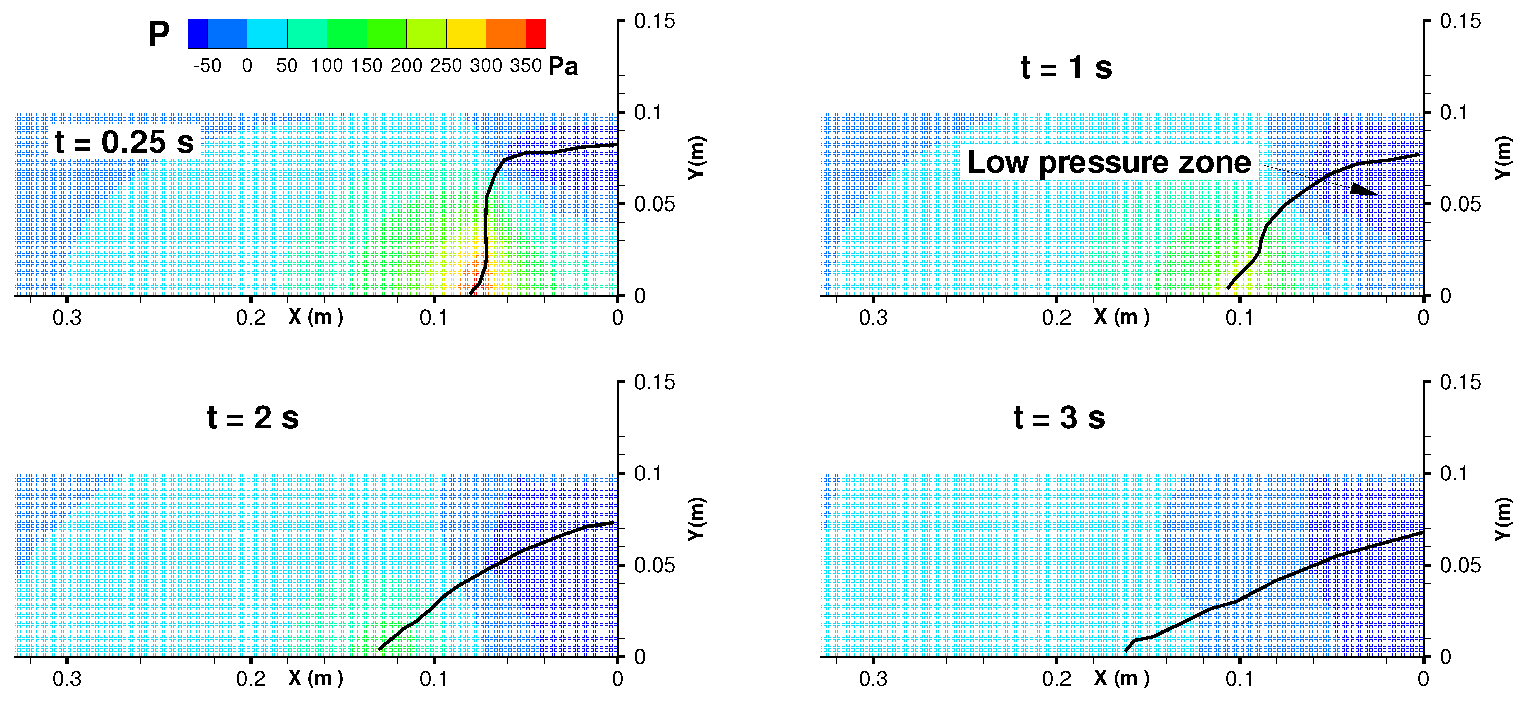
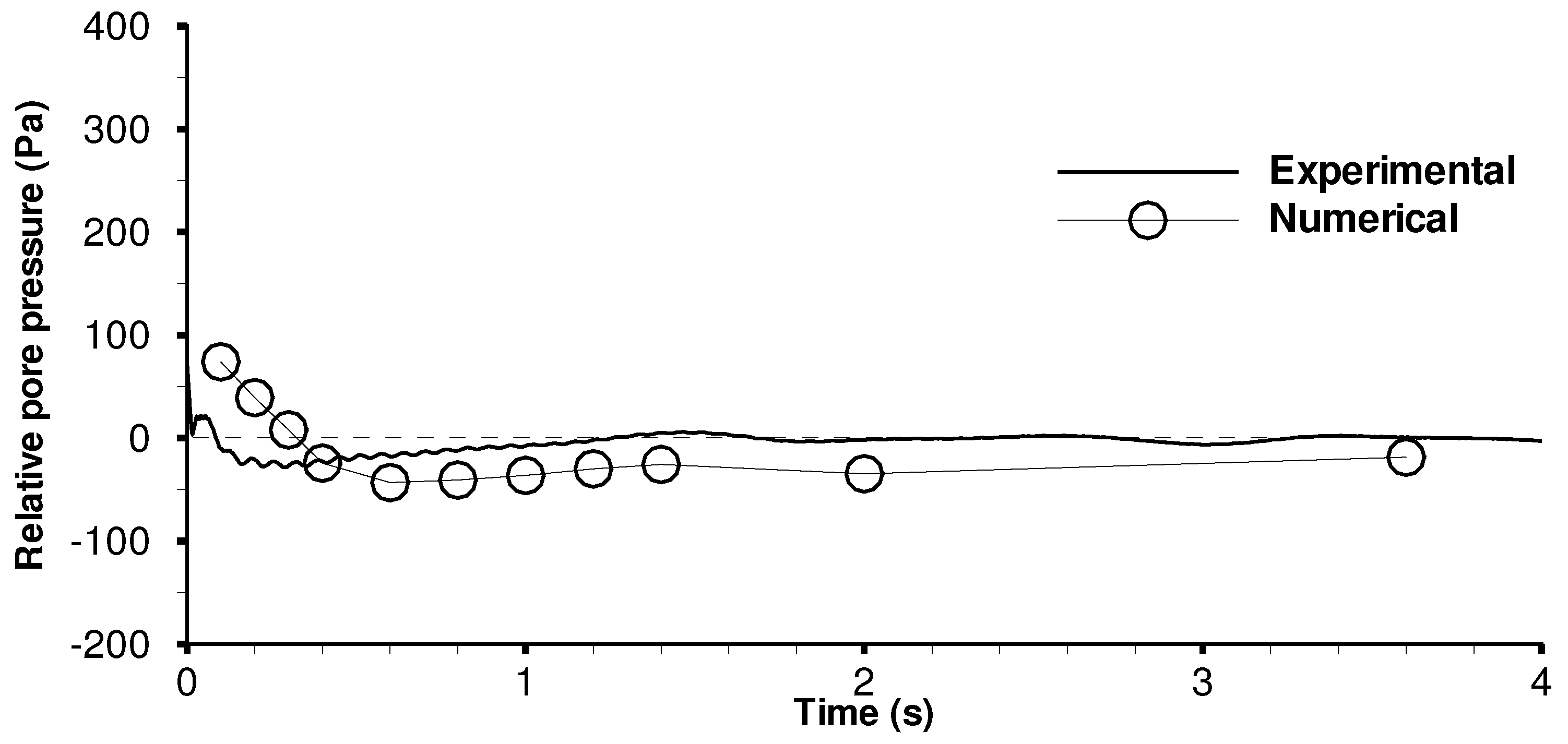
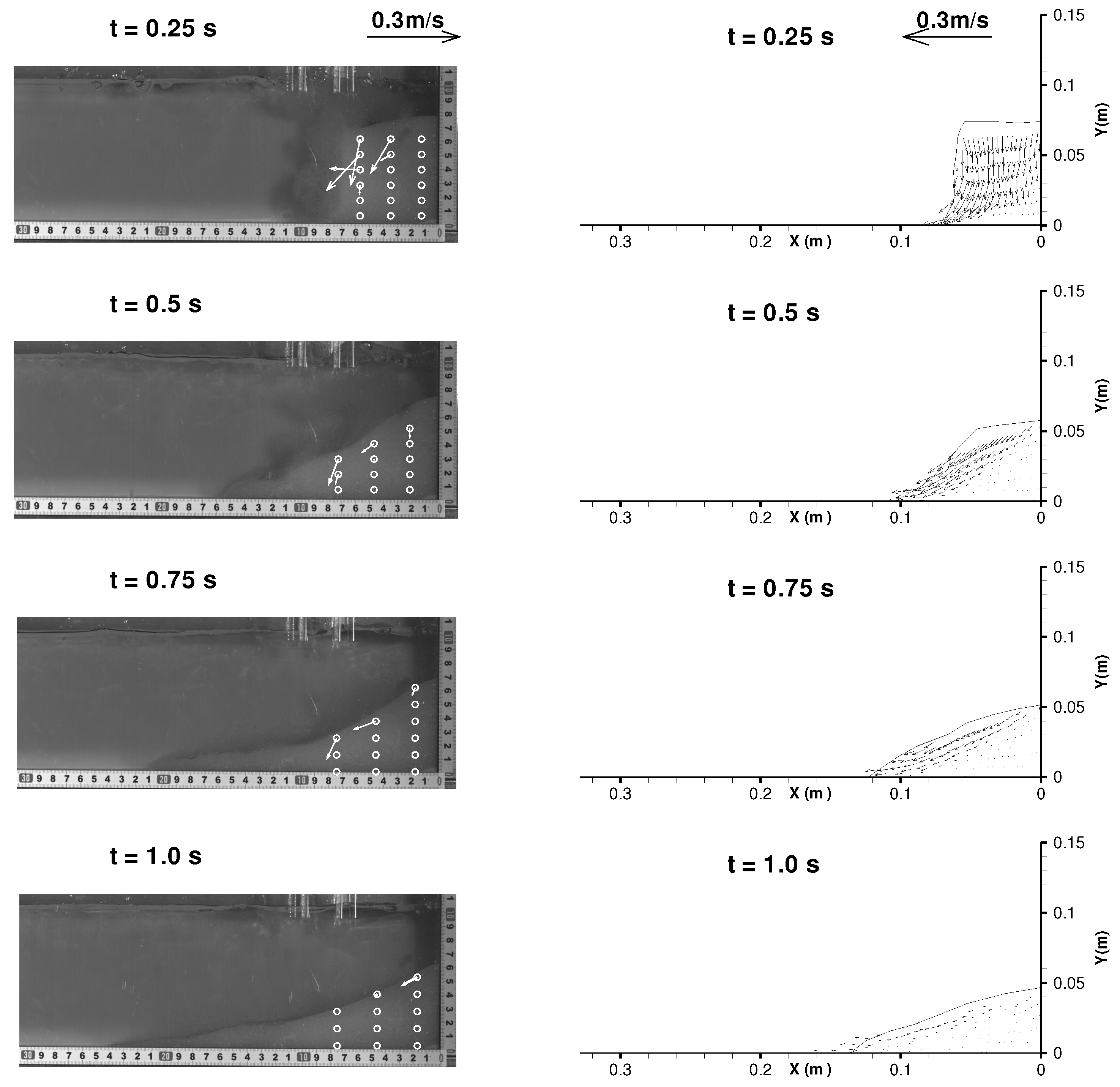
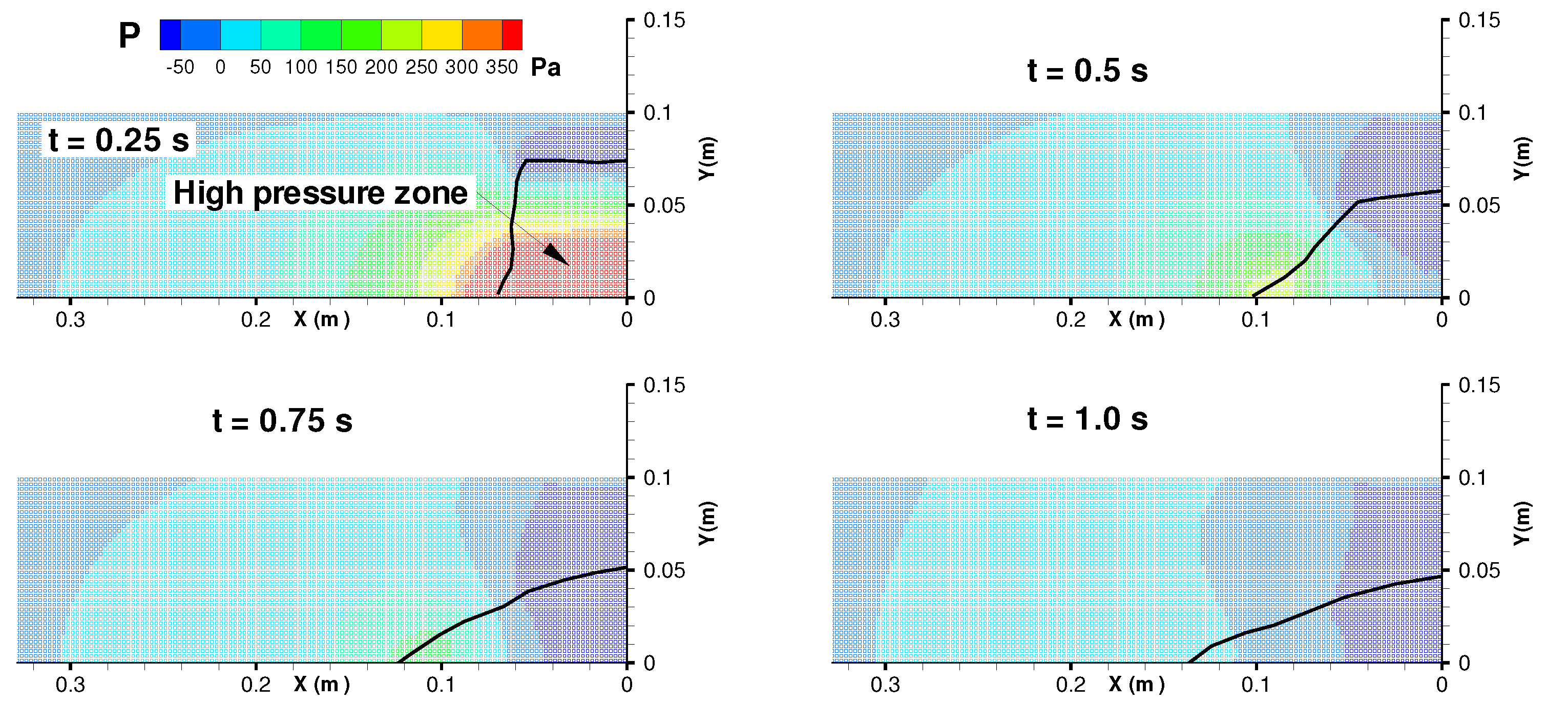
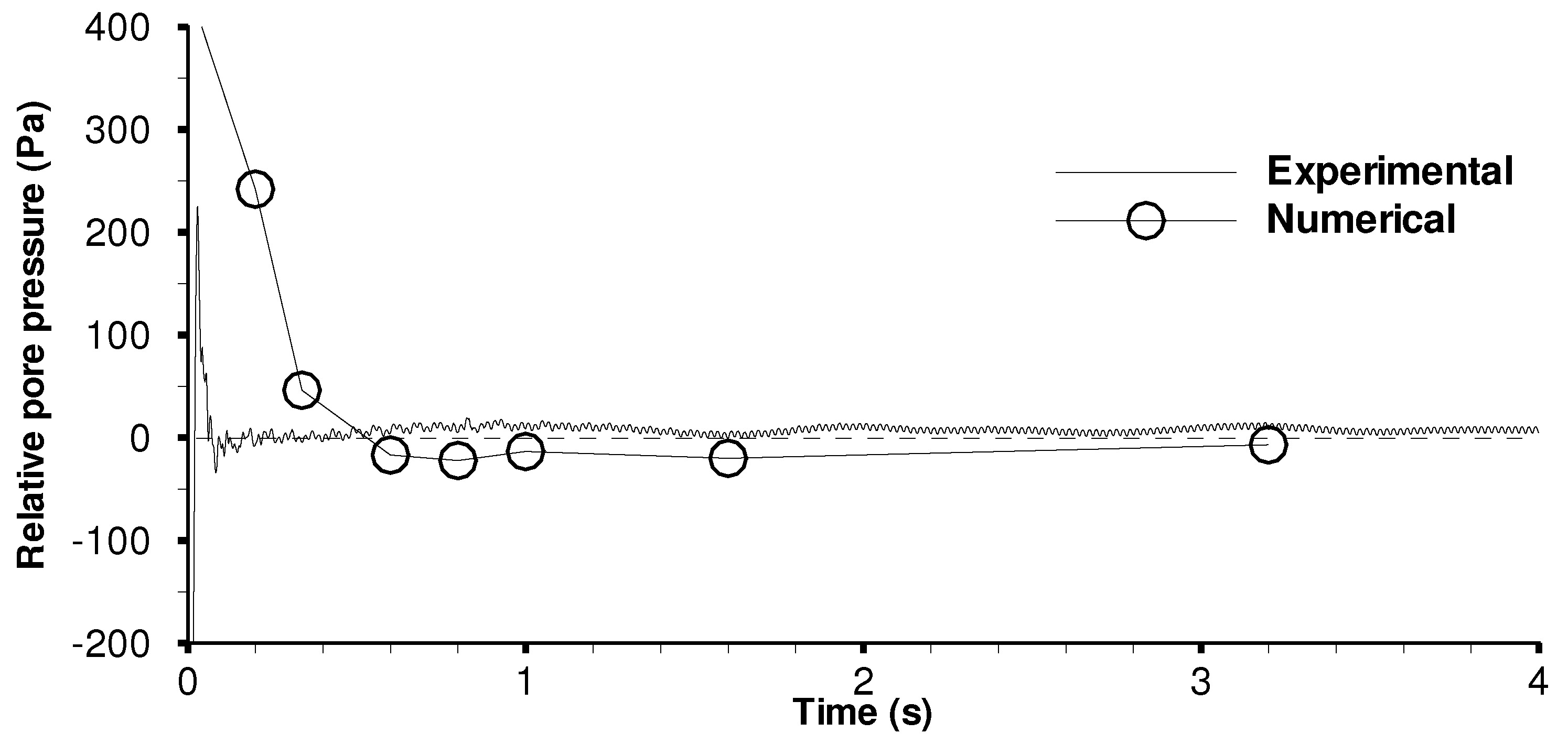
4.2. Submerged Granular Column Collapse

In this section, the submerged granular column collapse is simulated using the proposed coupled Eulerian–Lagrangian model for two-fluid mixture flows. Both initially dense and loose packing columns are considered in succession.

Figure 8 shows a rectangular tank of 0.50 m in length and 0.15 m in height. The initial water level in the tank is 0.1 m. The submerged granular column is $L_i$ long and $H_i$ high. At $t=0$, the gate is suddenly removed, and the column then collapses. The gate can be removed within 0.03 s. Although granular column collapse is known to be quite sensitive to the way the gate is removed, the effects of the gate movement on the granular motion and the surrounding fluid motion are ignored. Material properties used in the calculation are shown in

Table 2. Material properties for the simulation of an initial 6 cm × 8 cm ($L_i\times H_i$) granular column collapse in water.

Property	Symbol	Value
True density of granular material	${\tilde{\rho }}_s$	2700 $\mathrm{kg}/{\mathrm{m}}^3$
Young’s modulus of granular material	E	70 MPa
Poisson’s ration of granular material	$\nu$	0.3
Internal friction angle of granular material	$\theta$	${20}^{\circ }$
Cohesion of granular material	c	0
Initial volume fraction of granular material	${\varphi }_{s0}$	0.55 (loose), 0.60 (dense)
Hydraulic conductivity of granular material	k	0.005 m/s
Viscosity of the water	$\mu$	0.001 $\mathrm{Pa}·\mathrm{s}$
Initial true density of the water	${\tilde{\rho }}_{f0}$	1000 $\mathrm{kg}/{\mathrm{m}}^3$
Mean granular diameter (glass beads)	d	225 $\mathsf{\mu }$m

. Model experiments of the same scale are also conducted to validate our numerical simulations. The experimental setup is the same as that in [13], but with a pressure sensor mounted on the side wall of the tank to measure the pore water pressure at point $P_1$. The position of the pressure sensor is shown in Figure 8. The sensor used is an HM91 micro pore pressure sensor and transducer produced by HELM SENSOR. The measuring range of this diffused silicon piezoresistive pressure sensor is from 0 to 10 kPa, with a 24 V DC power supply. The overall accuracy is $\pm 0.1\%FS$ (Full Scale). The loose packing is made by gently pouring the spherical glass beads into the reservoir delimited by the removable gate. To create dense packing columns, we gently tap on the tank wall. By doing so, the solid volume fraction reached in our setup is $0.55\pm 0.005$ for the immersed loose packing and $0.60\pm 0.003$ for the immersed dense packing. The solid volume fraction is measured and calculated by the displacement method. The diameter of the spherical glass beads ranges from 150 $\mathsf{\mu }$m to 300 $\mathsf{\mu }$m, with an average diameter of 225 $\mathsf{\mu }$m and standard deviation of 40 $\mathsf{\mu }$m.

There are a total of 9600 Eulerian cells and 3072 SPH particles for water and solid phase in the tank, respectively. The initial particle spacing is 0.00125 m. The grid size is twice as that of the solid particle interval, which means there are nearly four solid particles in one cell. Thus, the support domain of a solid particle should be doubled in order to contain more grid nodes. Numerical parameters are chosen as follows: Virtual speed of sound for water $c_f$ = 10 $\mathrm{m}/\mathrm{s}$; speed of sound for granular material $c_s$ = 150 $\mathrm{m}/\mathrm{s}$; artificial viscosity parameters $\alpha =0.1$, $\beta =0$; the artificial diffusive parameter in $\delta$-SPH method $\delta =0.1$ for SPH simulation of solid phase; for the repulsive force, $D=0.01$ and $r_0=0.00125$ m; time step size $\mathsf{\Delta }t=2.5\times {10}^{-6}$ s, which satisfies the constraints in (33). The non-associated flow rule with dilatancy angle $\psi$ determined by (23) and (24) is implemented in the calculation. For the meaning of some of the above parameters, see [12].

4.3. Dense Packing Column Collapse

Submerged granular column collapse can cause free surface waves. Figure 9 shows the free surface indicated by the water volume fraction ${\varphi }_f$, where ${\varphi }_f=0$ in the air domain, ${\varphi }_f=1$ in the pure water domain and $0<{\varphi }_f<1$ in the water–grain mixture. Here it should be pointed out that although the VOF function F is used to indicate the water free surface in the Eulerian domain, we combine F and ${\varphi }_f$ together and show the water free surface and solid surface simultaneously using ${\varphi }_f$ only, as seen in Figure 9. It is seen that the collapse of the submerged granular column leads to the sinkage of the water free surface above. The magnitude of the sinkage of the water free surface is in the order of 1cm, which agrees well with the experimental observations. Thus, the proposed numerical model has the capability of simulating free surface flows caused by underwater granular column collapse.

The granular column profile indicated by the water volume fraction ${\varphi }_f$ is also shown in Figure 9 which resolves the water volume fraction within the column and at its surface. Here, it should be pointed out that the granular surface is, in fact, a surface where ${\varphi }_f$ changes rapidly across it. In our numerical model, the water volume fraction ${\varphi }_f$ is calculated by interpolating the water volume fraction ${\varphi }_a$ (i.e., Equation (32)) on the Lagrangian solid particles to the Eulerian grid points using the SPH re-normalized interpolation approach (i.e., Equation (27)). Usually, in SPH simulation, a transition zone of ${\varphi }_f$ at the granular surface develops, due to the incompleteness of the support domain of the SPH interpolation function at the interface. However, as seen in Figure 9, due to the re-normalized interpolation technique used in this study, the transition zone is limited in a narrow space, namely the abrupt change of the volume fraction ${\varphi }_f$ at the interface is maintained.

We investigate the effectiveness of the special treatment of the pore water pressure mentioned in (31). Figure 10 shows some solid particles expelled out from the granular column by the improper treatment of the pore water pressure, i.e., Equation (30). Particle expelling results in the enlargement of the particle intervals. Consequently, a large transition zone of the water volume fraction ${\varphi }_f$ is formed and the pore water pressure in this zone cannot be predicted correctly. This instability, previously reported by [25], can be avoided by introducing $p^{\prime }$ in the approximation of the pore pressure gradient, as seen in (31). The main idea behind this treatment is to address the importance of the pressure difference, instead of the pressure itself, in the approximation of the pore water pressure gradient. With this treatment, the movement of the solid particles and the evolution of the water volume fraction ${\varphi }_f$ are stable, as seen in Figure 9.

Figure 11 shows the snapshots from both experimental observations and numerical simulations of an initially dense packing submerged granular column collapse. The granular velocity fields at representative times from the experiments and simulations are given for comparison. The experimental velocity fields of the solid phase are obtained by the software package Photoinfor which can capture the deformation patterns and analyzing the evolution of the deformation quantitatively (Li et al. [26]) by means of the so-called digital speckle correlation method (DSCM). The snapshots on the left column of Figure 11 are from experimental observations with arrows representing the velocity vectors of the granular particles they start on at a certain instant. It is seen that upon removal of the gate, particle movement takes place mainly at the upper left corner where the particles fall off the pile with a large velocity. After that, the particles mainly move along the granular surface layer and a “hydraulic-like granular jump” can be observed due to the stoppage of the slow-moving particles at downstream. The same phenomena are observed from the numerical simulations, except the discrepancy on the runout distance which may be due to the sparseness of particles at the surge front. Both experimental observation and numerical simulation show that the collapse of the initially dense packing column is finished within about 3 s.

Figure 12 shows the water pressure field at some representative times for an initially dense packing granular column collapse. Dense packing granular material exhibits dilation when sheared. As a result of the dilation, the interstitial pore water is sucked into the column, giving rise to a negative pore pressure field. In Figure 12, the hydrostatic pressure has been subtracted and only the dynamic deviation of the pore pressure is shown. That would make the low-pressure zone much more obvious. It is seen from Figure 12 that a lower pressure zone in the shearing zone develops at the initial stage of the dense column collapse. During the later stage of the collapse, this negative pressure field dissipates and recovers to the hydrostatic pressure due to the pore water infiltration.

To investigate the time evolution of the pore water pressure quantitatively, pore water pressure at point $P_1$ is investigated experimentally and numerically. Figure 13 shows the predicted relative pore water pressure at point $P_1$ compared with the experimental measurements. Here, “relative” means the pressure difference from the hydrostatic pressure of the surrounding fluid at the same depth. Experimental measurements show that at the initial stage, say $0<t<1$, a negative pressure is measured, and then it is recovered to the hydrostatic pressure during the later stage of the collapse. The fluctuations in the experimental pore pressure signal are due to the sloshing of the water free surface in the tank caused by the removing of the gate. Numerical pore water pressure shows the same trend, but the negative pressure appears later than in the experiments. The reason may be also due to the gate removing duration.

4.4. Loose Packing Column Collapse

Now we investigate the loose packing case. The initially loose packing column collapse shows some different scenarios. In Figure 14, the granular velocity fields obtained for an initially loose packing column is shown. It is seen that upon removal of the gate, the upper part of the column drops quickly, resulting in a surge of the front. After that, a thin layer of surface particles flows down a mild slope. Both experimental observation and numerical simulation show that the collapse of the initially dense packing column of this case is finished within about 1.5 s, much shorter than in the case of dense packing collapse. The experiments of [8] revealed that the collapse of an initially loose granular column can be finished within a few seconds, while for an initially dense granular column, the collapse can last for a much longer time, e.g., tens of seconds. Moreover, the runout distance of loose columns is twice longer than that of dense columns. Please note that [8] used a kind of very sticky liquid ($\mu$ = 0.012 Pa·s) in the experiments. Thus, the difference between our results and the experimental observations of [8] may be due to the fluid viscosity, which should be a good topic for the future.

Figure 15 shows the relative pore pressure field evolving during the collapse of an initially loose packing granular column. It is seen that due to the compaction of the loose packing, a high-pressure zone develops in the granular column at the initial stage of the collapse. For loose column collapse, a positive pore pressure can be measured below the column. Here, positive pressure is relative to the hydrostatic pressure of the surrounding fluid at the same depth. After that, the pore pressure dissipates and restores to the hydrostatic pressure in a short period. Figure 16 shows the predicted relative pore water pressure at point $P_1$ compared with the experimental measurements. Experimental measurements show that at the initial stage, say about $0<t<0.2$ s, a positive pressure is observed, and then it is recovered to the hydrostatic pressure during the later stage of the collapse. Numerical pore water pressure shows the same trend, but the positive pressure lasts a longer time than in the experiments. Interestingly, overshoot and oscillation of the pore pressure can be seen from both numerical and experimental results. Please note that in the dilatancy model (24), $K_3$ is a rheology parameter which should be calibrated in practice. Thus, a well calibrated $K_3$ might be useful to obtain a more realistic pore pressure feedback mechanism. However, this should be clarified in the future.

5. Conclusions

In this paper, numerical simulation of submerged granular column collapse by means of a Eulerian–Lagrangian coupled method is presented. Conservation equations of mass and momentum for both phases (water and solid particles) are formulated, based on the mixture theory. The solid is considered to be an elastic–perfectly plastic material. A Drucker-Prager yielding function with associated and non-associated plastic flow rules, respectively, is employed to describe the elastic-plastic behavior of the solid particles. The critical state theory is combined to consider the dilatancy or compaction of the granular material when subjected to shear.

A Eulerian–Lagrangian coupled method is employed to solve the proposed two-fluid mixture model. In this method, the continuous phase is solved using the Eulerian finite volume method (FVM) with the free surface captured by the volume-of-fluid (VOF) technique. The dispersed phase is solved by the Lagrangian smoothed particle hydrodynamic method (SPH). The Eulerian grid is composed of rectangular uniform Cartesian cells. The granular is decomposed into many material particles. The key issue is the information transfer between the Eulerian grid nodes and the Lagrangian particles. In the present method, this transfer is accomplished using the SPH kernel function. A re-normalized interpolation technique and an alternative treatment of the pressure term in the momentum equation for solid are employed to reduce the numerical instability of the SPH simulation.

The dry granular column collapse is studied first using the proposed approach. We investigate the influence of the stiffness, internal friction angle and aspect ratio on the morphology of the deposit. It is found that the morphology of the deposit is mainly dependent on the internal friction angle and the aspect ratio. The stiffness of the solid particles, which is identified by the bulk modulus of the solid material, has little effects on the granular deposit.

Compared with the dry granular column collapse, submerged granular column collapse exhibits many different features. For loose packing, the collapse process takes within a second; whereas dense packing can retard the flow significantly. Dilatancy (compaction) effects on the formation of different regimes is investigated. Agreement between our numerical simulations and experimental observations is good.In many situations, such as the underwater landslides, it is necessary to consider the effects of the ambient water on the mixture movements. The proposed coupled approach in this paper can deal with such problems widely occurred in underwater engineering and science.

References

1. Iverson, R.M. The physics of debris flows. Rev. Geophys. 1997, 35, 245–296. [Google Scholar] [CrossRef] [Green Version]
2. Legros, F. The mobility of long-runout landslides. Eng. Geol. 2002, 63, 301–331. [Google Scholar] [CrossRef]
3. Hampton, M.A.; Lee, H.J.; Locat, J. Submarine landslides. Rev. Geophys. 1996, 34, 33–59. [Google Scholar] [CrossRef]
4. Pelinovsky, E.; Poplavsky, A. Simplified model of tsunami generation by submarine landslides. Phys. Chem. Earth 1996, 21, 13–17. [Google Scholar] [CrossRef]
5. Pailha, M.; Pouliquen, O. A two-phase flow description of the initiation of underwater granular avalanches. J. Fluid Mech. 2009, 633, 115–135. [Google Scholar] [CrossRef]
6. Meruane, C.; Tamburrino, A.; Roche, O. On the role of the ambient fluid on gravitational granular flow dynamics. J. Fluid Mech. 2010, 648, 381–404. [Google Scholar] [CrossRef]
7. Meruane, C.; Tamburrino, A.; Roche, O. Dynamics of dense granular flows of small-and-large-grain mixtures in an ambient fluid. Phys. Rev. E 2012, 86, 026311. [Google Scholar] [CrossRef]
8. Rondon, L.; Pouliquen, O.; Aussillous, P. Granular collapse in a fluid: Role of the initial volume fraction. Phys. Fluids 2011, 23, 073301. [Google Scholar] [CrossRef] [Green Version]
9. Topin, V.; Monerie, Y.; Perales, F.; Radjaï, F. Collapse dynamics and runout of dense granular materials in a fluid. Phys. Rev. Lett. 2012, 109, 188001. [Google Scholar] [CrossRef] [Green Version]
10. Savage, S.; Babaei, M.; Dabros, T. Modeling gravitational collapse of rectangular granular piles in air and water. Mech. Res. Commun. 2014, 56, 1–10. [Google Scholar] [CrossRef]
11. Si, P.; Shi, H.; Yu, X. Development of a mathematical model for submarine granular flows. Phys. Fluids 2018, 30, 083302. [Google Scholar] [CrossRef]
12. Wang, C.; Wang, Y.; Peng, C.; Meng, X. Smoothed particle hydrodynamics simulation of water-soil mixture flows. J. Hydraul. Eng. 2016, 142, 04016032. [Google Scholar] [CrossRef] [Green Version]
13. Wang, C.; Wang, Y.; Peng, C.; Meng, X. Dilatancy and compaction effects on the submerged granular column collapse. Phys. Fluids 2017, 29, 103307. [Google Scholar] [CrossRef]
14. Wang, C.; Wang, Y.; Peng, C.; Meng, X. Two-fluid smoothed particle hydrodynamics simulation of submerged granular column collapse. Mech. Res. Commun. 2017, 79, 15–23. [Google Scholar] [CrossRef]
15. Yuan, Q.; Wang, C.; Wang, Y.; Peng, C.; Meng, X. Investigation of submerged soil excavation by high velocity water jet using two-fluid smoothed particle hydrodynamics method. J. Hydraul. Eng. 2019, 145, 04019016. [Google Scholar] [CrossRef]
16. Chen, F.; Qiang, H.; Zhang, H.; Gao, W. A coupled SDPH-FVM method for gas-particle multiphase flow: Methodology. Int. J. Numer. Methods Eng. 2016, 109, 73–101. [Google Scholar] [CrossRef]
17. Hirt, C.; Nichols, B. Volume of fluid (vof) method for the dynamics of free boundaries. J. Comput. Phys. 1981, 39, 201–225. [Google Scholar] [CrossRef]
18. Bui, H.H.; Fukagawa, R.; Sako, K.; Ohno, S. Lagrangian meshfree particles method (SPH) for large deformation and failure flows of geomaterial using elastic-plastic soil constitutive model. Int. J. Numer. Anal. Methods Geomech. 2008, 32, 1537–1570. [Google Scholar] [CrossRef]
19. Pailha, M.; Nicolas, M.; Pouliquen, O. Initiation of underwater granular avalanches: Influence of the initial volume fraction. Phys. Fluids 2008, 20, 111701. [Google Scholar] [CrossRef]
20. Andreotti, B.; Forterre, Y.; Pouliquen, O. Granular Media: Between Fluid and Solid; Cambridge University Press: Cambridge, UK, 2013. [Google Scholar]
21. Iverson, R.M. Landslide triggering by rain infiltration. Water Resour. Res. 2000, 36, 1897–1910. [Google Scholar] [CrossRef] [Green Version]
22. Iverson, R.M. Regulation of landslide motion by dilatancy and pore pressure feedback. J. Geophys. Res. 2005, 110. [Google Scholar] [CrossRef]
23. Crespo, A.; Gómez-Gesteira, M.; Dalrymple, R.A. Boundary conditions generated by dynamic particles in sph methods. Comput. Mater. Continua. 2007, 5, 173–184. [Google Scholar]
24. Lube, G.; Huppert, H.E.; Sparks, R.S.J.; Freundt, A. Collapses of two-dimensional granular columns. Phys. Rev. E 2005, 72, 1301–1310. [Google Scholar] [CrossRef] [PubMed] [Green Version]
25. Bui, H.H.; Fukagawa, R.; Sako, K.; Wells, J. Slope stability analysis and discontinuous slope failure simulation by elasto-plastic smoothed particle hydrodynamics (SPH). Geotechnique 2011, 61, 565–574. [Google Scholar] [CrossRef]
26. Li, Y.; Lin, Z.; Jing, H.; Yang, S. High-accuracy digital speckle correlation method for rock with dynamic fractures. Chin. J. Geotech. Eng. 2012, 34, 1060–1068. (In Chinese) [Google Scholar]
Figure 1. Domain discretization.
Jmse 09 00617 g001
Figure 2. Interpolation strategy between Eulerian grid nodes and Lagrangian particles. Staggered grid for the Eulerian variables is illustrated. Left: Grid information transfer to a certain particle; Right: Transfer of particles information to the grid nodes. A square-type cell system (same Δ x , Δ y sides) is used here. k h is the radius of the support domain of a solid particle or a grid node, h is the initial distance between solid particles and k is a constant normally in the range from 2 to 4. A larger value of k implies more particles in the support domain.
Jmse 09 00617 g002
Figure 3. Dry granular column collapse in air.
Jmse 09 00617 g003
Figure 4. Influence of the internal friction angle θ on the morphology of the deposit for dry granular column collapse. Soil profiles at t = 0.5 s are plotted.
Jmse 09 00617 g004
Figure 5. The final slope of a dry granular column collapse with different Young’s modulus E.
Jmse 09 00617 g005
Figure 6. Dry granular column collapse with different aspect ratios ( a = H i / L i = 0.1 / 0.1 , 0.2 / 0.1 , 0.3 / 0.1 , 0.1 / 0.2 , respectively).
Jmse 09 00617 g006
Figure 7. Numerical simulations of dry granular column collapse with and without continuity Equation (1). The slope profile at t = 0.3 s is shown. The initial granular column is 0.1 m wide and 0.2 m high.
Jmse 09 00617 g007
Figure 8. Submerged granular column collapse. D w is the water depth. L i and H i are the initial length and height of the granular column, respectively.
Jmse 09 00617 g008
Figure 9. Numerical results show the evolution of water free surface and granular profile indicated by the water volume fraction ϕ f at some representative times for the initially dense packing case.
Jmse 09 00617 g009
Figure 10. Numerical instability caused by the conventional SPH approximation of the pore water pressure gradient, i.e., Equation (30).
Jmse 09 00617 g010
Figure 11. Granular velocity fields at some representative times for the initially dense packing column collapse. Left column: experimental observations; Right column: numerical simulations.
Jmse 09 00617 g011
Figure 12. Numerical results show the relative pore water pressure field evolution during the collapse process of an initially dense packing submerged granular column.
Jmse 09 00617 g012
Figure 13. Relative pore water pressure at point P 1 during the collapse process of an initially dense packing granular column.
Jmse 09 00617 g013
Figure 14. Granular velocity field at some representative times for an initially loose packing column collapse. Left column: experimental observations; Right column: numerical simulations.
Jmse 09 00617 g014
Figure 15. Numerical results show the relative pore water pressure field evolution during the collapse process of an initially loose packing submerged granular column.
Jmse 09 00617 g015
Figure 16. Relative pore water pressure at point P 1 during the collapse process of an initially loose packing granular column.
Jmse 09 00617 g016