Maneuverability and Hydrodynamics of a Tethered Underwater Robot Based on Mixing Grid Technique

Abstract

The maneuverability and hydrodynamic performance of the tethered underwater robot in a uniform flow field is investigated. In this research, a tethered underwater robot symmetrically installed with NACA66 hydrofoils and Ka 4-70/19A ducted propellers around its main body is first constructed. The method of overlapping grid combined with sliding mesh is applied in the numerical simulations, and the principle of relative motion is adopted to describe the hydrodynamic responses of the tethered underwater robot during the robot manipulation. The reliability of the CFD methods applied in this research is verified by experimental results, and the comparison between numerical and experimental ones shows that there is very little difference being found. The numerical results indicate that computational cost due to the research’s large-scale domain can be effectively reduced by the adopted numerical methods, hydrofoils’ control effect is greatly influenced by the towing speeds, and thrusts issued from the ducted propellers are related to the tethered underwater robot’s position and towing speed.

1. Introduction

Many resources in the complex ocean environment can be widely explored by the tethered underwater robot because it can execute a lot of tasks in searching hydrologic features or observing the ocean environment [1]. A tethered underwater robot is usually composed of the robot’s main body, trajectory and attitude control equipment, and umbilical cable. Understanding the nature of an underwater robot coupling the effect of umbilical cable under different control operations is a complex task for scholars.

Methods to investigate the dynamic performances of a tethered underwater robot can be classified in two ways: experiment study and numerical simulation. The latter can be further sub-classified as the Finite Element Methods, Finite Difference Method [2], and Lump-Mass-Spring Formulation [3,4]. The experiment study is more reliable than numerical simulation, but it is time consuming, expensive, and cannot catch the details of the flow field around the tethered underwater robot. The numerical simulation depends significantly on the correctness of the proposed mathematic model to predict the hydrodynamic performance of the tethered underwater robot.

To discuss the hydrodynamic performance of umbilical cable, Ablow and Schechter proposed a three-dimensional model to simulate the motion of cable [2], Walton and Polachek presented a three-dimensional Lump-Mass formulation [4], and Chai et al. further added bending and torsional stiffness into the Lump-Mass formulation of cable [3]. Luis et al. investigated a towing cable model using a finite element method and validated the numerical result with experimental data [5]. Laranjeira proposed a novel visual servoing control scheme based on a parameterized cable model of the tether [6]. Palm and Eskilsson studied the influence of bending stiffness on snap loads in marine cables with a high-order discontinuous Galerkin method [7].

In studying the hydrodynamic performance of the tethered underwater robot’s main body, Li et al. discussed an underwater robot’s hydrodynamic characteristics with a novel technique so as to measure the hydrodynamic forces and moments in the experiment [8]. Zarei et al. utilized wind tunnel and finite volume method to study the hydrodynamic performance of the underwater robot [8].

Inspired by the problem of hydrodynamic performance of the tethered underwater robot, Wu and Chwang combined Ablow and Schechter’s method with the six-degrees-of-freedom equation of an underwater robot to study a two-part underwater towed system [9]. Wu et al. proposed an integrated hydrodynamics and control model coupling the undersea environment’s hydrological factors to simulate a tethered underwater robot system [10], and the result is validated by experiment [11]. Park et al. presented a numerical method adding bending stiffness in the low-tension cable to investigate the dynamic behavior of a towed underwater robot [12].

In investigating the algorism of planning tethered underwater robot’s trajectory, adaptive neural network, PID, and sliding mode algorisms are commonly used in the tethered underwater robot [13,14,15,16,17,18]. The implementation of the control operations is achieved by applying the external force from control devices in the robot to drive it along a given trajectory.

There are lots of reports to study the control equipment for the tethered underwater robot. Zhou and Zhao analyzed the effects of the deflection angle, rotational speed, and ducted propeller spacing on the underwater robot thrust performance [19]. Vu et al., investigated the motion of a tethered underwater robot installed with four propellers under different propeller’s rotational speeds [20]. Fang et al. took into account the effect of the umbilical cable on the underwater robot’s motion [21], and Wu et al. analyzed the thrust of ducted thruster propulsion for a tethered underwater robot in turning motion [22].

From the above discussions, it can be found that few current studies are concentrated on the maneuverability and hydrodynamic performance of the tethered underwater robot combined hydrofoils with ducted propellers. Although there is a multiple control method applied in the tethered underwater robot, the hydrodynamic performance of tethered underwater robots under the control of control equipment is paid less attention. However, the hydrodynamic performance of a tethered underwater robot’s main body is actually greatly influenced by the control equipment [23].

The work of this paper focuses on discussing the hydrodynamic performance of tethered underwater robots with control equipment. The influence between control equipment and the underwater robot is considered. In order to simulate the complex motion of the tethered underwater robot in the working environment, a valid CFD method based on the governing equation of flow field, cable, and six-degrees-of-freedom model is proposed. The method also utilizes CFD techniques, such as sliding mesh and an overlapping grid, to exchange flow field data and simulate the motion of the tethered underwater robot. In this research, a tethered underwater robot with hydrofoils and propellers is first constructed, and the whole computational domain of the flow field is divided into different small regions. The simulation of the rotation of control equipment is applied with the sliding mesh, and the hydrodynamic performance of the tethered underwater robot by controlling the swing of hydrofoils or the rotational speeds of propellers is investigated in the Simcenter Star-ccm+2020.1.

2. Numerical Method

2.1. The Governing Equations of Flow Field

The governing equations of the flow field around the underwater robot are assumed to be incompressible and can be written as:

$$\frac{\partial {\mathrm{u}}_{\mathrm{i}}}{\partial {\mathrm{x}}_{\mathrm{i}}}=0\left(\mathrm{i}=1,2,3\right)$$

(1)

$$\mathsf{\rho }\left[\frac{\partial {\mathrm{u}}_{\mathrm{i}}}{\partial \mathrm{t}}+\frac{\partial \left({\mathrm{u}}_{\mathrm{i}}{\mathrm{u}}_{\mathrm{j}}\right)}{\partial {\mathrm{x}}_{\mathrm{j}}}\right]=-\frac{\partial \mathrm{P}}{\partial {\mathrm{x}}_{\mathrm{i}}}+{\mathsf{\rho }\mathrm{g}}_{\mathrm{i}}+\mathsf{\rho }\frac{\partial }{\partial {\mathrm{x}}_{\mathrm{j}}}\left[\mathsf{\mu }\left(\frac{\partial {\mathrm{u}}_{\mathrm{i}}}{\partial {\mathrm{x}}_{\mathrm{j}}}+\frac{\partial {\mathrm{u}}_{\mathrm{j}}}{\partial {\mathrm{x}}_{\mathrm{i}}}\right)-\overline{{\mathrm{u}}_{\mathrm{i}}^{’}{\mathrm{u}}_{\mathrm{j}}^{’}}\right]$$

(2)

where ${\mathrm{u}}_{\mathrm{i}}$, ${\mathrm{u}}_{\mathrm{j}}$, are the time-averaged value of the velocity component ($\mathrm{i},$$\mathrm{j}=1,2,3$); $\mathrm{P}$ is fluid pressure; $\mathsf{\rho }$ is the density of the fluid; $\mathrm{t}$ is the time; $\mathsf{\mu }$ is the viscosity; ${\mathrm{g}}_{\mathrm{i}}$ $\left(\mathrm{i}=1,2,3\right)$ is the component of gravity acceleration; and $-\mathsf{\rho }\overline{{\mathrm{u}}_{\mathrm{i}}^{’}{\mathrm{u}}_{\mathrm{j}}^{’}}$ is the Reynolds stress term, which is solved by a realizable $\mathrm{k}-\mathsf{\epsilon }$ turbulence model [24]. The turbulent kinetic energy Equation (3) and turbulent dissipation Equation (4) are shown as follows:

$$\frac{\partial }{\partial \mathrm{t}}\left(\mathsf{\rho }\mathrm{k}\right)+\frac{\partial }{\partial {\mathrm{x}}_{\mathrm{i}}}\left({\mathsf{\rho }\mathrm{ku}}_{\mathrm{j}}\right)=\frac{\partial }{\partial {\mathrm{x}}_{\mathrm{j}}}\left[\left(\mathsf{\mu }+\frac{{\mathsf{\mu }}_{\mathrm{t}}}{{\mathsf{\sigma }}_{\mathrm{k}}}\right)\frac{\partial \mathrm{k}}{\partial {\mathrm{x}}_{\mathrm{j}}}\right]+{\mathrm{G}}_{\mathrm{k}}+{\mathrm{G}}_{\mathrm{b}}-\mathsf{\rho }\mathsf{\epsilon }-{\mathrm{Y}}_{\mathrm{M}}+{\mathrm{S}}_{\mathrm{k}}$$

(3)

$$\begin{gathered} \frac{\partial }{\partial \mathrm{t}}\left(\mathsf{\rho }\mathsf{\epsilon }\right)+\frac{\partial }{\partial {\mathrm{x}}_{\mathrm{j}}}\left({\mathsf{\rho }\mathsf{\epsilon }\mathrm{u}}_{\mathrm{j}}\right)=\frac{\partial }{\partial {\mathrm{x}}_{\mathrm{j}}}\left[\left(\mathsf{\mu }+\frac{{\mathsf{\mu }}_{\mathrm{t}}}{{\mathsf{\sigma }}_{\mathsf{\epsilon }}}\right)\frac{\partial \mathsf{\epsilon }}{\partial {\mathrm{x}}_{\mathrm{j}}}\right]+{\mathsf{\rho }\mathrm{C}}_1\mathrm{S}\mathsf{\epsilon }-{\mathsf{\rho }\mathrm{C}}_2\frac{{\mathsf{\epsilon }}^2}{\mathrm{k}+\sqrt{\mathrm{v}\mathsf{\epsilon }}} \\ +{\mathrm{C}}_{1\mathsf{\epsilon }}\frac{\mathsf{\epsilon }}{\mathrm{k}}{\mathrm{C}}_{3\mathsf{\epsilon }}{\mathrm{G}}_{\mathrm{b}}+{\mathrm{S}}_{\mathsf{\epsilon }} \end{gathered}$$

(4)

where $\mathsf{\eta }=\mathrm{S}\frac{\mathrm{k}}{\mathsf{\epsilon }}$, $\mathrm{S}=\sqrt{2{\mathrm{S}}_{\mathrm{ij}}{\mathrm{S}}_{\mathrm{ij}}}$; $\mathrm{k}$ is the turbulent kinetic energy and $\mathsf{\epsilon }$ is the turbulent dissipation; ${\mathrm{G}}_{\mathrm{k}}$ indicates the generation of turbulence kinetic energy due to the mean velocity gradients; ${\mathrm{G}}_{\mathrm{b}}$ is the generation of turbulence kinetic energy due to buoyancy; ${\mathrm{Y}}_{\mathrm{M}}$ represents the contribution of fluctuating dilatation in compressible turbulence to the overall dissipation rate; ${\mathrm{C}}_2$ and ${\mathrm{C}}_{1\mathsf{\epsilon }}$ are constants; ${\mathsf{\sigma }}_{\mathrm{k}}$ and ${\mathsf{\sigma }}_{\mathsf{\epsilon }}$, respectively, are the turbulent Prandtl numbers for $\mathrm{k}$ and $\mathsf{\epsilon }$; ${\mathrm{S}}_{\mathrm{k}}$ and ${\mathrm{S}}_{\mathsf{\epsilon }}$ are source terms.

2.2. The Governing Equations of the Underwater Robot

In order to compute the translational and angular motion of the tethered underwater robot, the governing equations for six degrees of the underwater robot in the local coordinate system are given as follows [25]:

$$\mathrm{m}\left[\dot{\mathrm{u}}-\mathrm{vr}+\mathrm{wq}-{\mathrm{x}}_{\mathrm{G}}\left({\mathrm{q}}^2+{\mathrm{r}}^2\right)+{\mathrm{y}}_{\mathrm{G}}\left(\mathrm{pq}- \dot{\mathrm{r}}\right)+{\mathrm{z}}_{\mathrm{G}}\left(\mathrm{pr}+\dot{\mathrm{q}}\right)\right]=\mathrm{X}$$

(5)

$$\mathrm{m}\left[\dot{v}-\mathrm{ur}-\mathrm{wp}+{\mathrm{x}}_{\mathrm{G}}\left(\mathrm{pq}+\dot{r}\right)-{\mathrm{y}}_{\mathrm{G}}\left(p^2+r^2\right)+{\mathrm{z}}_{\mathrm{G}}\left(\mathrm{qr}-\dot{\mathrm{p}}\right)\right]=\mathrm{Y}$$

(6)

$$\mathrm{m}\left[\dot{\mathrm{w}}-\mathrm{uq}+\mathrm{vp}+{\mathrm{x}}_{\mathrm{G}}\left(\mathrm{pr}-\dot{\mathrm{q}}\right)+{\mathrm{y}}_{\mathrm{G}}\left(\mathrm{qr}+\dot{\mathrm{p}}\right)-{\mathrm{z}}_{\mathrm{G}}\left({\mathrm{p}}^2+{\mathrm{q}}^2\right)\right]=\mathrm{Z}$$

(7)

$$\begin{gathered} {\mathrm{I}}_{\mathrm{x}}\dot{\mathrm{p}}+\left({\mathrm{I}}_{\mathrm{z}}-{\mathrm{I}}_{\mathrm{y}}\right)\mathrm{qr}+{\mathrm{I}}_{\mathrm{xy}}\left(\mathrm{pr}-\dot{\mathrm{q}}\right)-{\mathrm{I}}_{\mathrm{yz}}\left({\mathrm{q}}^2-{\mathrm{r}}^2\right)-{\mathrm{I}}_{\mathrm{xz}}\left(\mathrm{pq}+\dot{\mathrm{r}}\right)+ \\ \mathrm{m}\left[{\mathrm{y}}_{\mathrm{G}}\left(\dot{\mathrm{w}}-\mathrm{uq}+\mathrm{vp}\right)-{\mathrm{z}}_{\mathrm{G}}\left(\dot{\mathrm{v}}+\mathrm{ur}-\mathrm{wp}\right)\right]=\mathrm{K} \end{gathered}$$

(8)

$$\begin{gathered} {\mathrm{I}}_{\mathrm{y}}\dot{\mathrm{q}}+\left({\mathrm{I}}_{\mathrm{x}}-{\mathrm{I}}_{\mathrm{z}}\right)\mathrm{pr}-{\mathrm{I}}_{\mathrm{xy}}\left(\mathrm{qr}-\dot{\mathrm{p}}\right)+{\mathrm{I}}_{\mathrm{yz}}\left(\mathrm{pq}-\dot{\mathrm{r}}\right)+{\mathrm{I}}_{\mathrm{xz}}\left({\mathrm{p}}^2-{\mathrm{r}}^2\right)- \\ \mathrm{m}\left[{\mathrm{x}}_{\mathrm{G}}\left(\dot{\mathrm{w}}-\mathrm{uq}+\mathrm{vp}\right)-{\mathrm{z}}_{\mathrm{G}}\left(\dot{\mathrm{u}}-\mathrm{vr}+\mathrm{wq}\right)\right]=\mathrm{M} \end{gathered}$$

(9)

$$\begin{gathered} {\mathrm{I}}_{\mathrm{z}}\dot{\mathrm{r}}+\left({\mathrm{I}}_{\mathrm{y}}-{\mathrm{I}}_{\mathrm{x}}\right)\mathrm{pq}-{\mathrm{I}}_{\mathrm{xy}}\left({\mathrm{p}}^2-{\mathrm{q}}^2\right)-{\mathrm{I}}_{\mathrm{yz}}\left(\mathrm{pr}+\dot{\mathrm{q}}\right)+{\mathrm{I}}_{\mathrm{xz}}\left(\mathrm{qr}-\dot{\mathrm{p}}\right)+ \\ \mathrm{m}\left[{\mathrm{x}}_{\mathrm{G}}\left(\dot{\mathrm{v}}+\mathrm{ur}-\mathrm{wp}\right)-{\mathrm{y}}_{\mathrm{G}}\left(\dot{\mathrm{u}}-\mathrm{vr}+\mathrm{wq}\right)\right]=\mathrm{N} \end{gathered}$$

(10)

In Equations (5)–(10), is the mass of the underwater robot; the equations of left are comprised of inertia forces and moments, while the equations of right represent external forces and moments of the underwater robot; $\left({\mathrm{x}}_{\mathrm{G}},{\mathrm{y}}_{\mathrm{G}},{\mathrm{z}}_{\mathrm{G}}\right)$ is the barycenter of the underwater robot; ${\mathrm{I}}_{\mathrm{x}}$, ${\mathrm{I}}_{\mathrm{y}}$ and ${\mathrm{I}}_{\mathrm{z}}$ are the inertia moments of mass; ${\mathrm{I}}_{\mathrm{xy}}$, ${\mathrm{I}}_{\mathrm{yz}}$ and ${\mathrm{I}}_{\mathrm{xz}}$ are the polar inertia moments of the underwater robot;$\left(\dot{\mathrm{u}},\dot{\mathrm{v}},\dot{\mathrm{w}}\right)$, $\left(\dot{\mathrm{p}},\dot{\mathrm{q}},\dot{\mathrm{r}}\right)$ are the translational and angular accelerations of the underwater robot, respectively; $\left(\mathrm{X},\mathrm{Y},\mathrm{Z}\right)$ and $\left(\mathrm{K},\mathrm{M},\mathrm{N}\right)$ are external forces and moments on the underwater robot. The paper focuses on the tethered underwater robot’s motion in the x-z plane, which is controlled by the hydrofoils and ducted propellers. The tethered underwater robot’s roll, swing, and yaw is restricted, which means that Y,$\mathrm{K}$,$\mathrm{N}$ is zero.

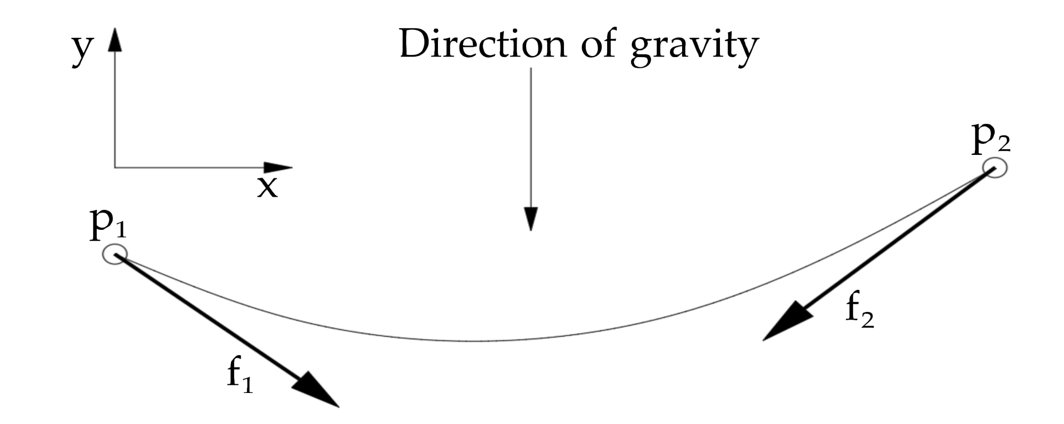
2.3. The Governing Equations of the Cable

The cable coupling model applied in this paper is elastic, quasi-stationary and subjected to its weight in the gravity field, which connects between the underwater robot at the lower end of the cable and the working ship at the upper end of the cable. The equation of the shape of the cable is expressed as:

$$\mathrm{x}=\mathrm{an}+\mathrm{bsin}\mathrm{h}\left(\mathrm{n}\right)+\mathsf{\alpha },{ \mathrm{n}}_1\le \mathrm{n}\le {\mathrm{n}}_2$$

(11)

$$\mathrm{y}=\mathrm{acos}\mathrm{h}\left(\mathrm{n}\right)+\frac{\mathrm{b}}{2}{\sin \mathrm{h}}^2\left(\mathrm{n}\right)+\mathsf{\beta },{\mathrm{n}}_1\le \mathrm{n}\le {\mathrm{n}}_2$$

(12)

$$\mathrm{a}=\frac{\mathrm{c}}{{\mathsf{\lambda }}_0\mathrm{g}}, \mathrm{b}=\frac{\mathrm{ca}}{{\mathrm{DL}}_{\mathrm{eq}}},\mathrm{c}=\frac{{\mathsf{\lambda }}_0{\mathrm{L}}_{\mathrm{eq}}\mathrm{g}}{\sin \mathrm{h}\left({\mathrm{u}}_2\right)-\sin \mathrm{h}\left({\mathrm{u}}_1\right)}$$

(13)

Equations (11)~(13) describe the shape of the cable. In the equations, $\mathrm{x}$, $\mathrm{y}$ are the coordinate of the cable; $\mathrm{g}$ is the gravitational acceleration; ${\mathsf{\lambda }}_0$ and ${\mathrm{L}}_{\mathrm{eq}}$ are the mass per unit length and the relaxation length of the cable under force-free conditions; $\mathrm{D}$ is the stiffness of the cable; $\mathsf{\alpha }$ and$\mathsf{\beta }$, are integration constants depending on the position of the two end points and the total mass of the cable. and  are integration constants depending on the position of the two end points and the total mass of the cable. The curve parameter $\mathrm{u}$ is related to the inclination angle of the cable curve, and the parameter values ${\mathrm{n}}_1$ and ${\mathrm{n}}_2$ represent the positions of the cable’s endpoint ${\mathrm{p}}_1$ and ${\mathrm{p}}_2$, as shown in Figure 1. The force of the cable applying on the endpoints ${\mathrm{p}}_1$ and ${\mathrm{p}}_2$ is decomposed to the x and y-direction as follows:

$${\mathrm{f}}_{1,\mathrm{x}}=\mathrm{c},{\mathrm{f}}_{1,\mathrm{y}}=\mathrm{csin}\mathrm{h}\left({\mathrm{n}}_1\right)$$

(14)

$${\mathrm{f}}_{2,\mathrm{x}}=-\mathrm{c},{\mathrm{f}}_{2,\mathrm{y}}=-\mathrm{csin}\mathrm{h}\left({\mathrm{n}}_1\right)$$

(15)

where the forces ${\mathrm{f}}_1$ and ${\mathrm{f}}_2$ acting on the two endpoints of the cable are directed along the tangent vectors of the cable curve at the parameter values n₁and n₂.

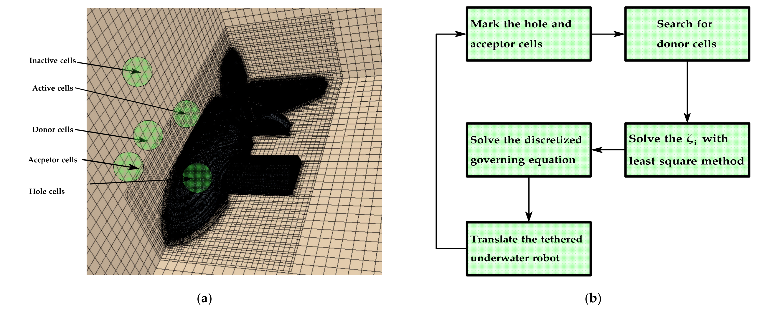
2.4. The Sliding Mesh

To describe the hydrodynamics of propeller rotation motion, a domain is set around the propeller in the underwater robot using the sliding mesh technique. In this research, a cylinder rotation domain (Domain I) with the sliding mesh technique and overset domain (Domain II) with the overlapping grid technique are constructed separately. The surface of the cylinder domain served as the non-conformal sliding interface that connects Domain I with Domain II, and it transfers the flow field information from one domain to another. The key to ensuring the consistency of flow field information is to keep the flow flux equal and the new interface due to the motion of mesh at every time step. The general conservation equation formulation for sliding mesh is calculated as follows:

$$\frac{\mathrm{d}}{\mathrm{dt}}\int \mathsf{\rho }\mathsf{\Phi }\mathrm{dV}+\int \mathsf{\rho }\mathsf{\Phi }\left(\overrightarrow{\mathrm{v}}-\overrightarrow{{\mathrm{v}}_{\mathrm{g}}}\right)\mathrm{dA}={{\displaystyle \int }}_{\partial \mathrm{V}}\mathsf{\Gamma }\nabla \mathsf{\Phi }\mathrm{d} \overrightarrow{\mathrm{A}}+{{\displaystyle \int }}_{\mathrm{V}}{\mathrm{S}}_{\mathsf{\Phi }}\mathrm{dV}$$

(16)

where $\mathsf{\rho }$ is the density of the fluid; $\overrightarrow{\mathrm{v}}$ is the flow velocity vector; $\overrightarrow{{\mathrm{v}}_{\mathrm{g}}}$ is the sliding mesh velocity;$\mathsf{\Gamma }$ is the diffusion coefficient; ${\mathrm{S}}_{\mathsf{\Phi }}$ is the source term of $\mathsf{\Phi }$; $\mathrm{V}$ is arbitrary control volume; $\mathsf{\Phi }$ is an integral form of the conservation equation for a general scalar.

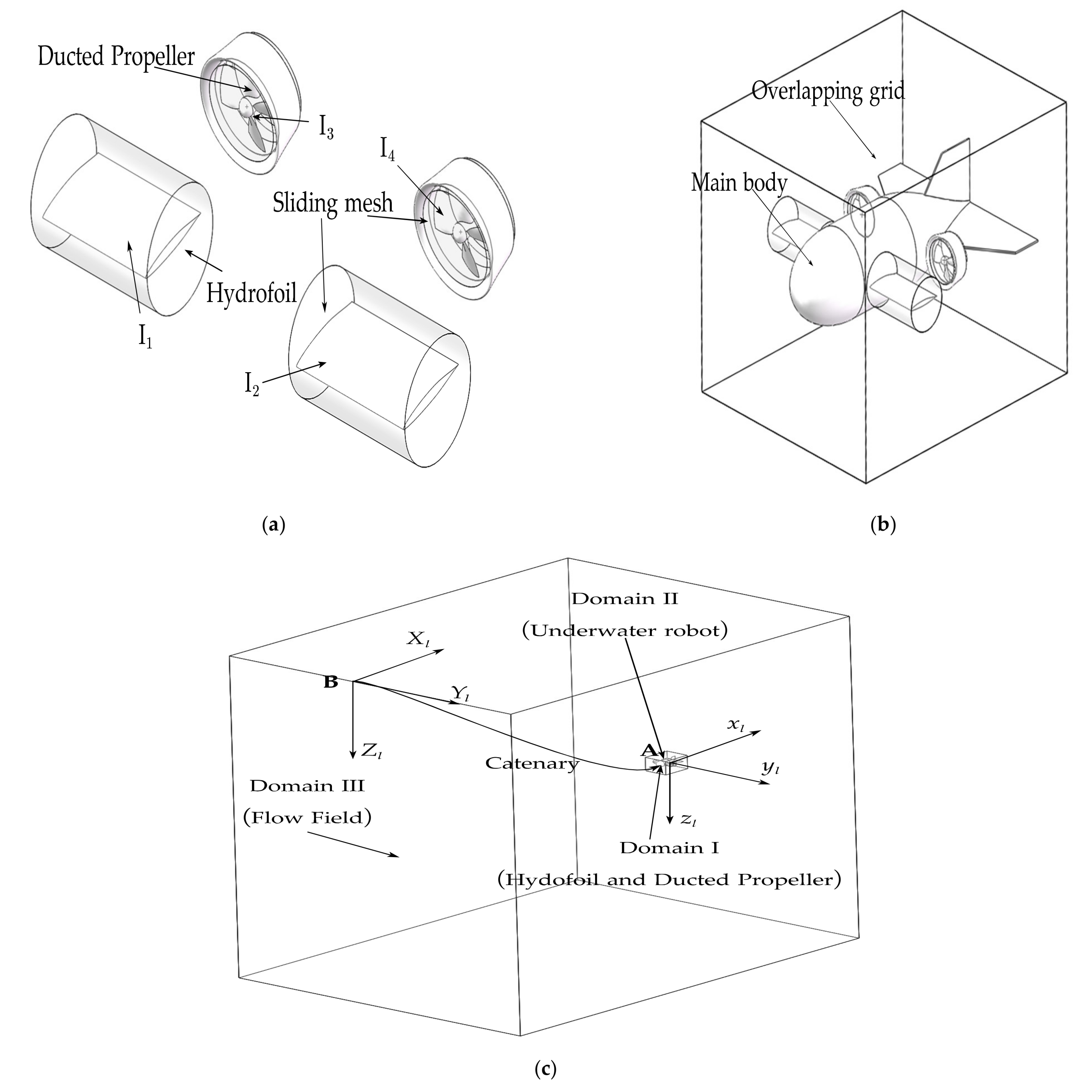
2.5. The Overlapping Grid

The overlapping grid is utilized to discretize a computational domain with different meshes, including the background region and overset region. The background region (Domain III) and overset region (Domain II) generate meshes, respectively. The process of numerical simulation requires the domain connectivity information about the mesh of Domains II and III, which includes different types of cells and the interpolation weights. The overlapping cells for the robot are grouped into multiple cell types: active cells, inactive cells, hole cells, and acceptor cells, as shown in Figure 2a. The governing equations are solved by the active cells, while no equation needs to be solved in the inactive cells. The inactive cells can change their status into active when the overset region approaches it. The hole cells lie in the underwater robot’s interior region, and it is used to mark the position of the robot so as to ensure the acceptor cell’s position. The acceptor cells separate the whole cells into active cells and inactive cells. The donor cells that lie around the acceptor cells provide acceptor cells with the interpolated information. The specific calculation procedure is shown in Figure 2b. In order to ensure high accuracy, the calculation is adopted least squares interpolation. The active cells in the flow field simultaneously solve, and the value of acceptor cells is acquired from the interpolation of multiple donor cells. The acceptor cells are calculated as follows:

$${\mathsf{\gamma }}_{\mathrm{I}}={\displaystyle \sum }_{\mathrm{i}=1}^{\mathrm{n}}{\mathsf{\zeta }}_{\mathrm{i}}{\mathsf{\gamma }}_{\mathrm{i}}$$

(17)

$${\displaystyle \sum }_{\mathrm{i}=1}^{\mathrm{n}}{\mathsf{\zeta }}_{\mathrm{i}}=1$$

(18)

where ${\mathsf{\zeta }}_{\mathrm{i}}$ represents the interpolation nondimensional coefficient for ${\mathsf{\gamma }}_{\mathrm{i}}$; ${\mathsf{\gamma }}_{\mathrm{I}}$ is the value of the acceptor cell; ${\mathsf{\gamma }}_{\mathrm{i}}$ is the value of the donor cell.

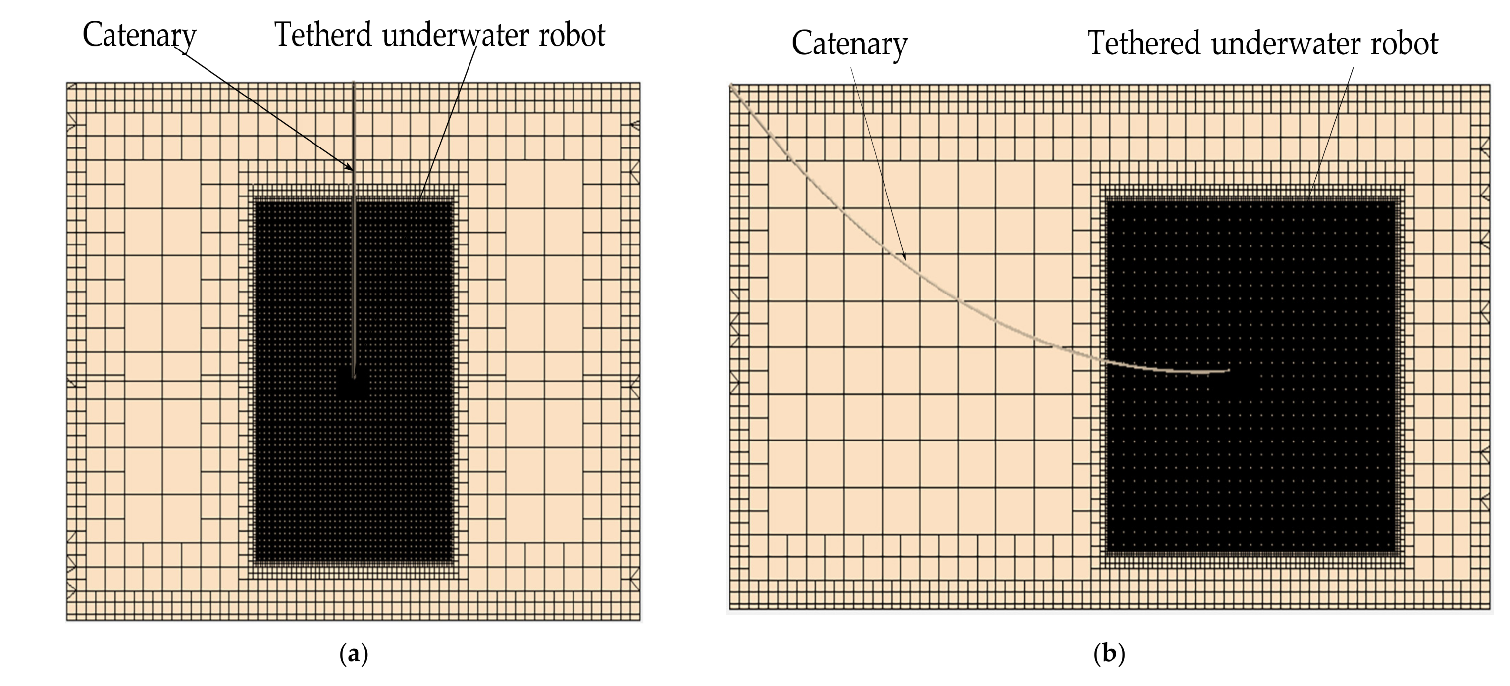
3. Numerical Computation Setup

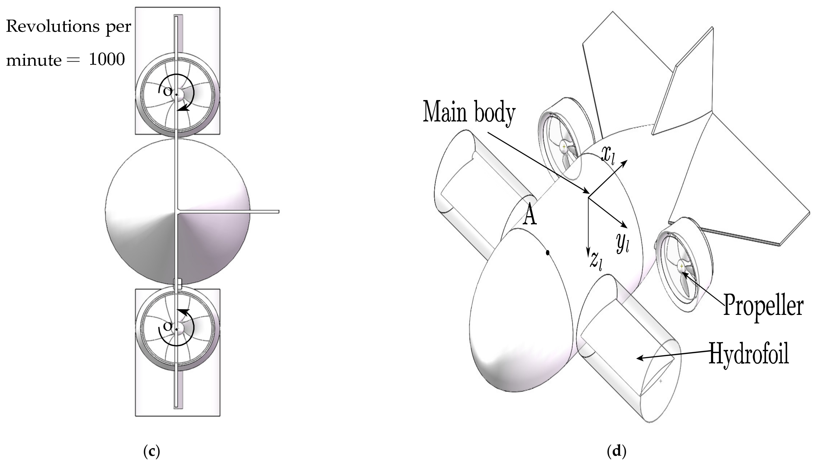
3.1. Geometric Model of the Tethered Underwater Robot

The tethered underwater robot investigated in this paper installs with two ducted propellers and two hydrofoils symmetrically linked with umbilical cable at point A as shown in Figure 3. The type of the ducted propeller is Ka70/19A, whose geometric model is constructed according to the three-dimensional coordinate transformation formula [26]. Primary parameters of the tethered underwater robot in the research are presented in

Table 1. Primary parameters of the tethered underwater robot.

Main Dimensions of the Tethered Underwater Robot:
length = 0.330 m, width = 0.270 m, height = 0.140 m
Center of gravity in the local coordinate system:
XG= 0.187 m, YG = 0.000 m, ZG = 0.000 m
m = 1.873 kg
Ka 4-70/19A Propellers:
Diameter:    47.3 mm
Disk area ratio:    0.7
Pitch diameter ratio:     0.99
Leaf inclination:    8°
Hub diameter ratio:     0.18
The rotational speed:    1000 rpm
Origin of the propeller coordinates in the local coordinate system:
Left Propeller:     x1 = 0.065 m, y1 = 0.080 m, z1 = 0 m
Right Propeller:−    x2 = 0.065 m, y2 =0.080 m, z2 = 0 m
NACA66 hydrofoils:
Chord:    50 mm
Span:    80 mm
Angle of attack:    −15°~15°
Camber ratio:    2%
Relative thickness    12%
Origin of the hydrofoil coordinates in the local coordinate system:
Left hydrofoil:    x3 = −0.060 m, y3 = 0.135 m, z3 = 0 m
Right hydrofoil:    x4 = −0.060 m, y4 = −0.135 m, z4 = 0 m
Towing cable:
Length:     6.0 m
Stiffness:    5000 N/m
Mass per unit length:     0.008 kg/m
Connecting points in the global coordinate system:
Point A:    xA = 5.500 m, yA = 0 m, zA = 3.000 m
Point B (the connecting point):     xB = 0 m, yB = 0 m, zB = 0 m

. The tethered underwater robot’s motion is driven by the control equipment installed in the robot, such as the hydrofoil providing heave force and the propellers producing the thrust to move forward. The rotation speed of ducted propellers is uniformly set at 1000 rpm. The swing of the hydrofoil with a period of 3 s is given by the scalar function:

$$\mathsf{\theta }=\frac{\mathsf{\pi }}{12}\sin \left(\frac{2\mathsf{\pi }}{3}\mathrm{t}\right)$$

(19)

where $\mathsf{\theta }$ is the attack angle of the hydrofoil, and $\mathrm{t}$ represents the time.

3.2. Determination of Computational Domain and Boundary

As depicted in Figure 4c, the integrated numerical domain applied in this paper is divided into several computational domains, including the domains of rotation for hydrofoils and propellers and the translation domain of the underwater robot. The different computational domains are connected by the interface technique that combines the separation domain and exchanges the data of the flow field in the different domains. The rotation simulation of propellers and hydrofoils is applied with the sliding mesh to set a rotational speed, and the motion simulation of the tethered underwater robot is carried out in the overlapping grid. To clearly understand the separated computational domains, the details of these regions are elaborated as follows:

Domain I: According to the motion requirement of the tethered underwater robot, Domain I is composed of Domain I_i (i = 1, 2, 3, 4) that represents ducted propellers and hydrofoils, respectively. As shown in Figure 4a, the Domain I_i is enclosed by the cylinder representing the rotation region with its diameter of 105% ducted propeller one, hydrofoil. The center axis of the cylinder is consistent with the rotation axis of the control equipment. It is noted that the rotational speeds of control equipment are, respectively, designated as the cylinder rather than control equipment, such as hydrofoils and propellers. On the basis of the technique of sliding mesh, it is equivalent to directly specify the rotational speed of the control equipment.

Domain II: The tethered underwater robot’s multiple degrees of freedom motion is realized by Domain II, as shown in Figure 4b. The boundary of Domain II is set as the overlapping grid to simulate the motion of the tethered underwater robot in the flow field. The dimensions of Domain II are set as 0.50 m (Length) × 0.40 m (Width) × 0.60 m (Height) and form the gap between the boundary of the overlapping grid and the surface of the tethered underwater robot so that the tethered underwater robot has enough overlapping region. The orphan cells are avoided in the process of calculation. For the purpose of ensuring the continuity of the flow field, the interfaces are designated between Domain I and Domain II.

Domain III: It is used to simulate the working environment of the tethered underwater robot, which includes Domain I and Domain II. The dimensions of Domain III are set as 8.00 m (Length) × 6.00 m (Width) × 4.00 m (Height). One of the cable’s endpoints is fixed at the top of Domain III, while the other endpoint is fastened in the tethered underwater robot. As

Table 2. Boundary conditions of the underwater robot.

Region	Geometry	Boundary Conditions
Domain I	Hydrofoils and Ducted propellers	Wall
Domain I and Domain II	The surfaces of the Cylinders	Interface
Domain II	The tethered underwater robot	Wall
Domain II	The cuboid includes the tethered underwater robot	Overlap grid
Domain II and Domain III	The surfaces of the cuboid	Overlap grid
Domain III	The surface of left and right, top and bottom	symmetry
Domain III	The surface of front	Velocity inlet
Domain III	The surface of back	Pressure outlet

displays, the boundary conditions are, respectively, specified in the surfaces of Domain III so that the numerical experiment can simulate different towing speeds in the numerical tank according to the principle of relative motion.

In order to decrease the computational cost and ensure the high accuracy of computation, the hexahedral mesh is chosen in the numerical simulation. The meshes of the computational domain are presented in

Table 3. Meshes of the computational domain.

Domain	Number of Meshes (m)	Minimum Size of Mesh (m)	Maximum Size of Mesh (m)
I	5.63 × 105	0.0025	1
II	9.41 × 105	0.0025	1
III	9.55 × 106	0.0025	1

, which shows the total computational cost. The mesh of numerical simulation is layer-by-layer refined around the tethered underwater robot so that the mesh density and mesh distribution are appropriate. The mesh refinement of the trajectory of the tethered underwater robot in Domain III is performed so that it can satisfy the interpolation of the overlapping grid, as illustrated in Figure 5a,b. After the computational mesh is generated, the diagnostics of star-ccm+ 2020.1 is utilized to check the mesh validity, which ensures that the mesh of the numerical simulation is topologically valid and has no negative volume cells.

3.3. Coordinate Systems of the Tethered Underwater Robot

As shown in Figure 4c, there are two different coordinate systems in the numerical simulation, that is, the local coordinate system $\left(x_l,y_l,z_l\right)$ defined in the tethered underwater robot’s barycenter, and the global coordinate system $\left(X_g,Y_g,Z_g\right)$ fixed in the connecting point.

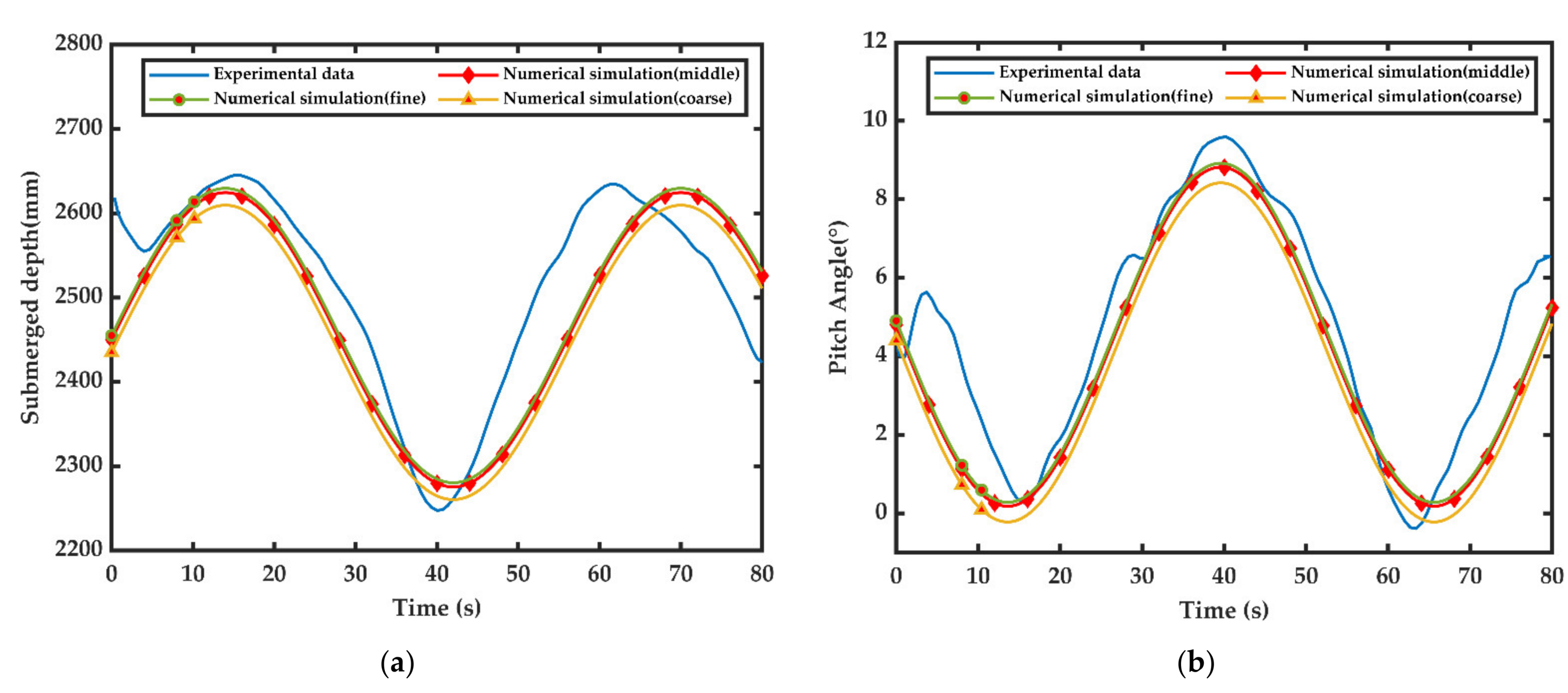
3.4. Validation of the Numerical Method with Experimental Results

In order to testify the validity of the proposed method to simulate the hydrodynamic behaviors of a tethered underwater robot, comparisons between the numerical results of a tethered underwater robot by the proposed numerical method in this paper and those of laboratory experiment [11] under the same conditions are presented. To ensure the accuracy of the validation, the geometric model is consistent with the experimental tethered underwater robot, which is composed of two hydrofoils to provide a depressing force for controlling the robot in heave motion and a streamline-shaped main body to maintain the robot in a stable towing attitude. In the towing tank, the tethered underwater robot connected by the nylon cable is towed at a constant velocity of 0.8 m/s. According to the principle of relative motion, the velocity inlet of numerical simulation is set at 0.8 m/s, which is equal to the tethered underwater towing velocity. Therefore, the large-scale flow field providing the tethered underwater robot’s motion is avoided, which reduces the massive calculation cost. The motion of the hydrofoil is set as $\mathsf{\theta }=\frac{\mathsf{\pi }}{18}\sin \left(\frac{2\mathsf{\pi }}{24}\mathrm{t}\right)$, which can be explained by the fact that the angle attack of the hydrofoil changes at the range of between −10 degrees and 10 degrees, and its period is 48 s. To ensure the mesh convergence, the computational domain is set with three different-sized meshes, including fine mesh with the number of 1.3 × 10⁷, middle mesh with the number of 1.1 × 10⁷, and coarse mesh with the number of 9.0 × 10⁶. The mesh sensitivity is applied in the overset region which includes the tethered underwater robot’s main body and control equipment, while the number of the mesh of flow field is kept the same. The base sizes of the overset region’s coarse mesh multiply 0.75 times and 0.50 times, respectively, to reach the middle and fine mesh. The base size will specify the reference length value for the overset region’s relative size controls of mesh.

Figure 6a,b presents the tethered underwater robot’s motion in the vertical plane. The data of the tethered underwater robot’s submerged depth and pitch angle curves present the same tendency compared with those of the experimental one. It can be found that the absolute error between the numerical and the experimental results gets smaller when the number of meshes increases. The numerical and experimental results show a bigger difference in the range of 0~15 s and 60~80 s. It is believed that the errors are caused by the following aspects: (1) the flow field is not stable at the initial situation, and the posture of the experimental prototype is influenced greatly by environmental factors when the towboat accelerates and decelerates; (2) the cable coupling model ignores the hydrodynamic force and only considers the gravity and tension, while the tethered underwater robot is towed by the nylon cable, which is influenced by the hydrodynamic force; (3) compared to the symmetrical numerical model, the experimental underwater robot is not totally symmetrical in its longitudinal section plane due to a manufacturing error; (4) for the requirement of simulating the hydrofoil’s rotation with sliding mesh, small parts of the geometric model connected with the hydrofoil are reduced.

To verify the mesh convergence, the relative errors for the same computational problem by applying a different number of meshes are analyzed. As shown in

Table 4. The comparison between numerical and experimental results at three sets of meshes.

	The Submerged Depth (mm)	The Relative Error	The Pitch Angle (°)	The Relative Error
Coarse (9 × 106)	2442.418	4.554%	8.415	12.262%
Middle (1.1 × 107)	2453.371	4.122%	8.813	8.111%
Fine (1.3 × 107)	2458.154	3.939%	8.855	7.673%
Experiment	2558.957	---	9.591	---

, the relative errors between the numerical results and experimental ones decrease with the rise in the number of meshes. There is only a 4.122% difference in maximum data error about the depth of the tethered underwater robot between the result of numerical simulation and the experimental one, while the comparison of the pitch angle shows an 8.111% difference in maximum data error when the number of meshes is 1.1 × 10⁷. When the number of meshes increases to 1.3 × 10⁷ from 1.1 × 10⁷, the numerical result shows little difference, which means that the middle number of meshes has reached the calculation accuracy requirement for tethered underwater robot’s motion. Considering the calculation cost, the middle number of meshes is adopted in the numerical simulation. Although the error of numerical result still exists, the submerged depth and pitch angle’s amplitude is close to the experimental data. From the above discussion, it is valid to utilize the numerical method to simulate the tethered underwater robot’s motion.

4. Results and Discussions

In this section, the tethered underwater robot coupling the rotation of the ducted propeller and the swing of hydrofoil is towed at different speeds in a uniform flow field. The tethered underwater robot is subjected to various forces, such as the force of hydrofoils, the fluid force of the main body, the tension and gravity of the cable, and the thrust of ducted propellers. The hydrodynamic performances of the tethered underwater robot, hydrofoils, cable, and ducted propellers are discussed qualitatively and quantitatively as follows. The calculation time for the numerical simulation of a condition at the middle number of meshes is 55 h, based on two CPU AMD EPYC^TM-7542 with 64 cores at 3.4 GHz.

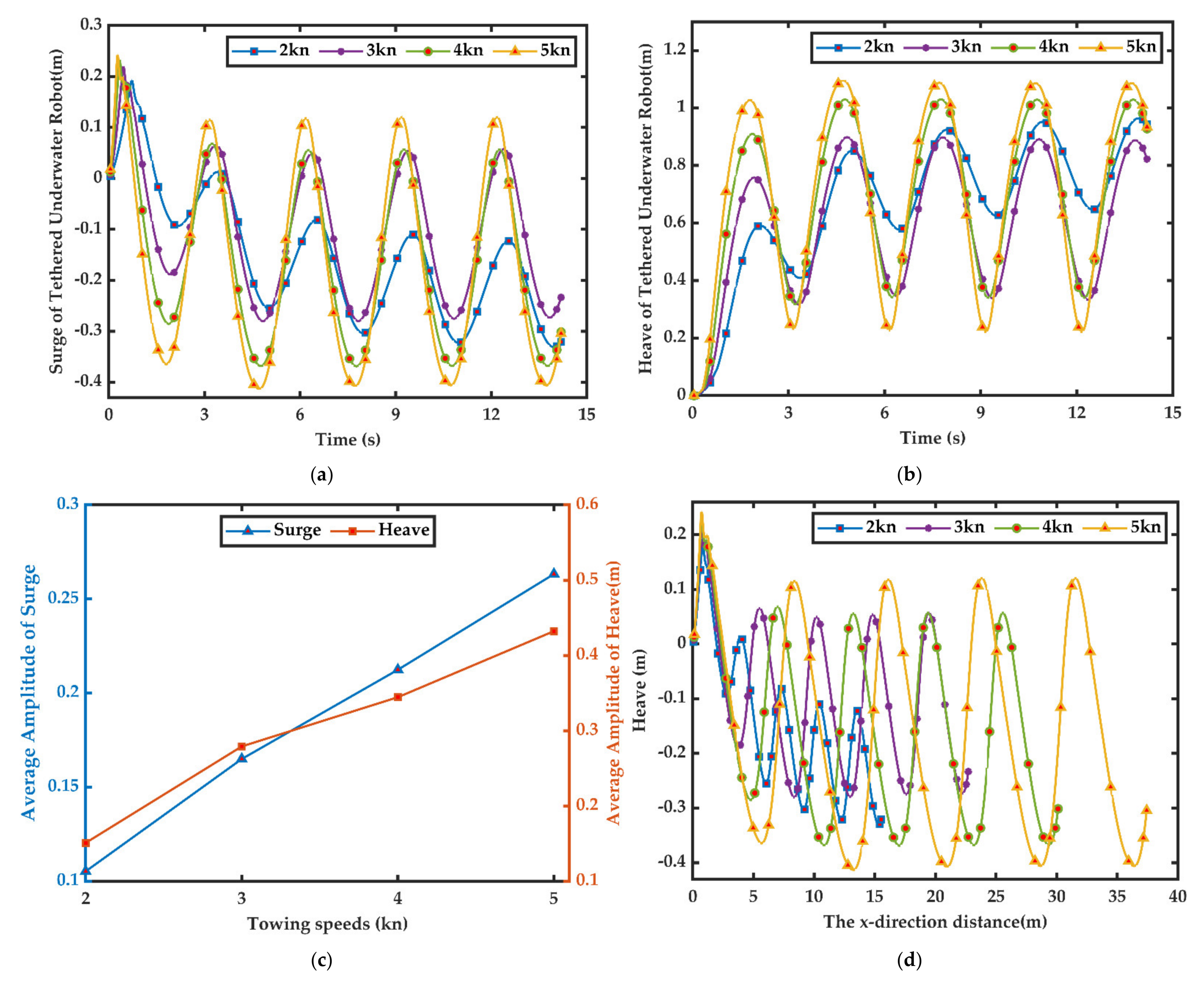
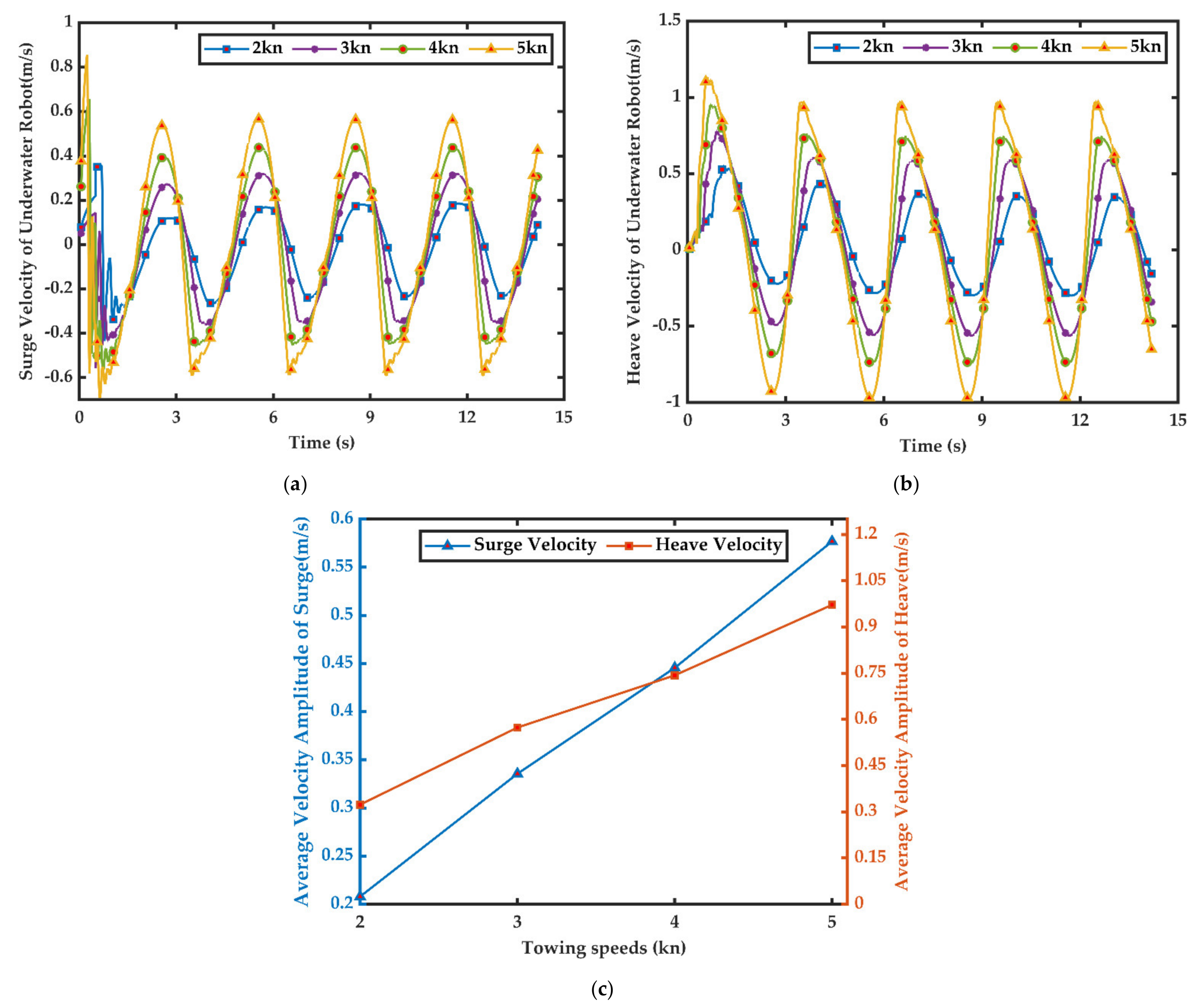
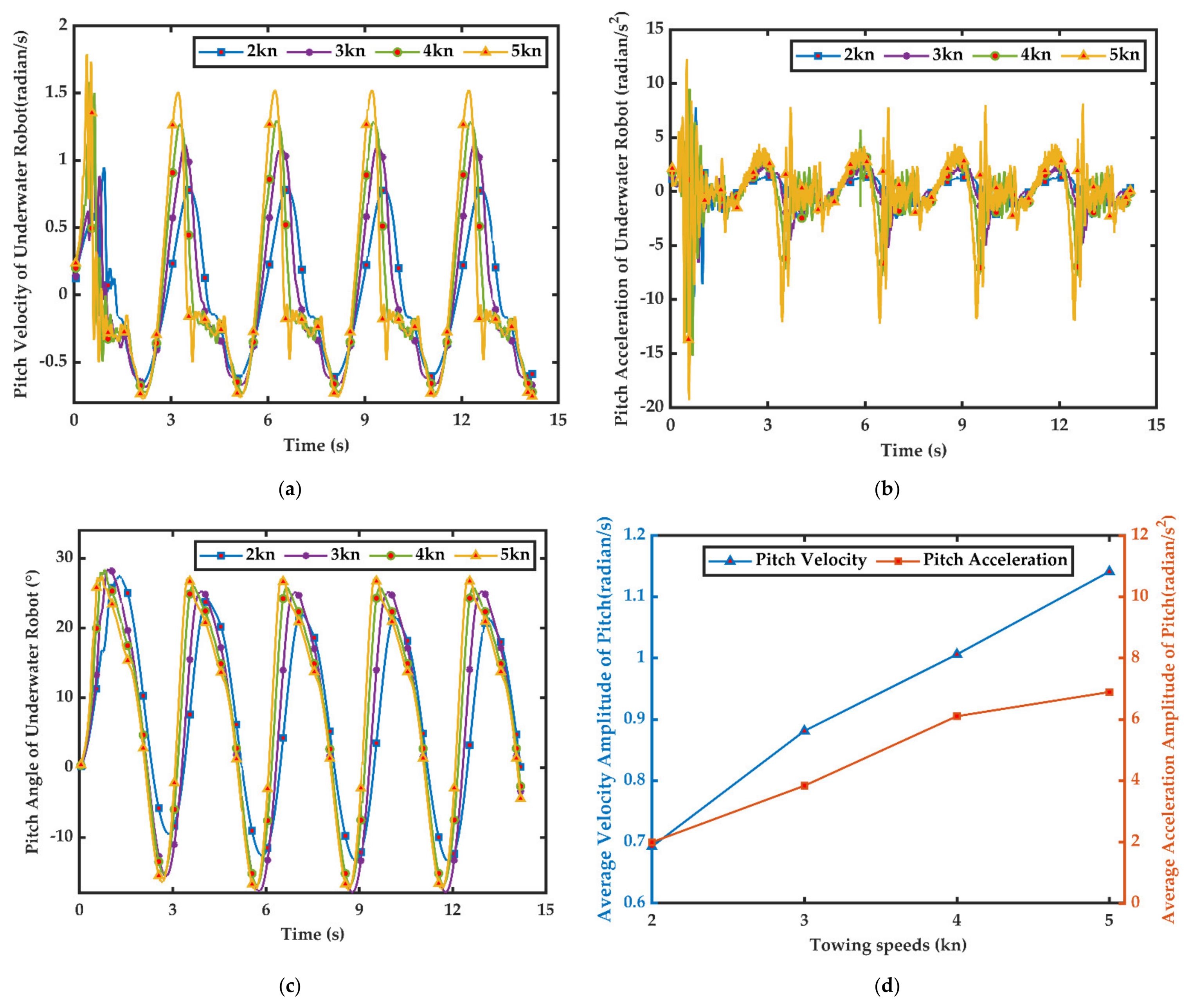
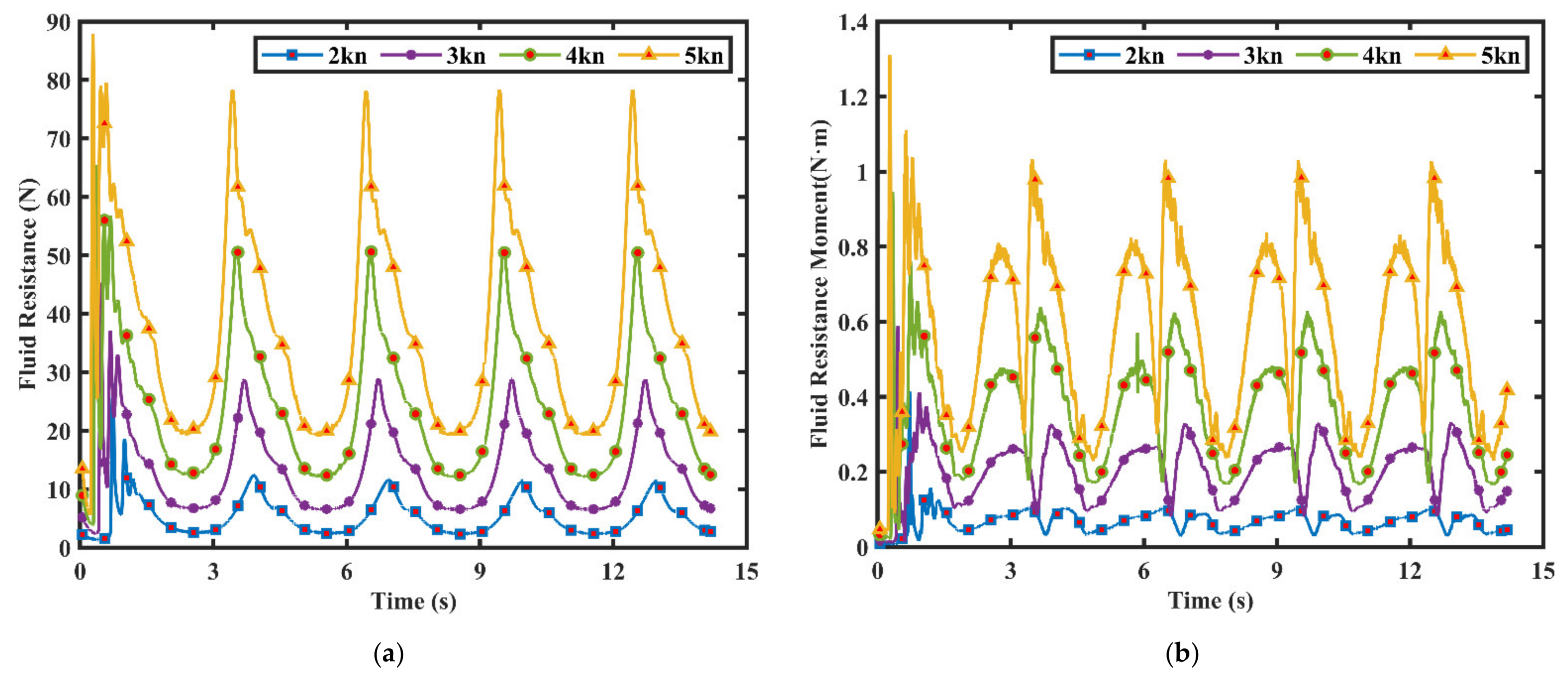
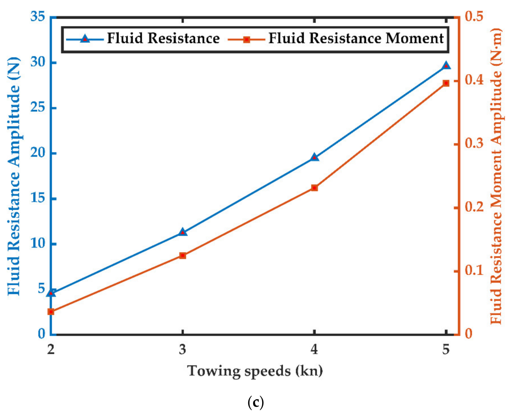
4.1. Trajectory and Hydrodynamic Performance of the Tetherd Underwater Robot

Figure 7a,b presents the time histories of the surge and heave of the tethered underwater robot at different towing speeds. The tethered underwater robot is driven in the positive x-direction, and the tethered underwater robot’s surge shows a growing tendency with the increase in towing speed. As illustrated in Figure 7c, the average amplitude of surge increases by 56.84% at 3 knots, 101.90% at 4 knots, and 150.29% at 5 knots, compared to the tethered underwater robot’s surge at 2 knots. The average amplitude of heave increases by 179.85% as the towing speed increases to 5 knots. These results suggest that the trajectory of the tethered underwater robot is mainly influenced by the towing speed. The growth of the tethered underwater robot’s surge is attributed to the tethered underwater robot’s heave and the fluctuation of relaxation length of cable. The cable with high stiffness has 6.0 m in length, and the cable’s endpoint on the tugboat is fixed. The cable’s endpoint on the tethered underwater robot moves to different locations when the tethered underwater robot heaves under the control of hydrofoil, which results in the variation of the relaxation of cable. The time histories of the trajectories of the tethered underwater robot at four constant towing speeds are shown in Figure 7d. The tethered underwater robot sinks at the start, and the axis of the heave is not the initial position of the tethered underwater robot, which indicates that the initial position is not a balanced state. The reason for the change of the tethered underwater robot’s position is the combined influence of the residual buoyancy, thrust from ducted propellers, and hydrofoils’ lift.

Figure 8a,b show the time histories of the surge and heave velocity components of the tethered underwater robot at different towing speeds. It is noted that the value of the surge velocity component fluctuates rapidly at the range of 0~1 s, which is caused by the disturbance of the unsteady flow field and the restriction of a cable. Figure 8c presents the relationship of average velocity amplitude of the tethered underwater robot in surge and heave motions with the towing speed. It can be found that the averaged velocity amplitude of surge and heave motions manifests a linear growing tendency with the towing speed increasing. The average value of surge velocity amplitude markedly enhanced by 61.38% at 3 knots, 114.33% at 4 knots, and 177.44% at 5 knots, compared to the surge’s velocity amplitude of the tethered underwater robot at 2 knots. The average velocity amplitude of heave significantly increases by 77.42% at 3 knots, 129.85% at 4 knots, and 200.62% at 5 knots, contrasting to the heave velocity amplitude of the tethered underwater robot at 5 knots. The pattern of the tethered underwater robot’s velocity is consistent with the trajectory of the tethered underwater robot.

Figure 9a–d illustrate the time history of the angular velocity of the robot and the relationship of pitch amplitude of the robot with towing speeds. From the figures, it can be found that there is a significant increase in the pitch amplitude when the towing speed increases. It is believed that the hydrodynamic effects of the hydrofoil on the robot make the pitch response of the robot quicken.

The time histories of the pitch acceleration of the robot at the different towing speeds are presented in Figure 9b. It can be seen that the fluctuation of the robot’s pitch acceleration is rapid, and the peak values in the pitch acceleration curve oscillate between −19.31 and 12.25 N when towing speed increases to 5 knots. The reason for the rapid fluctuation in the curve is mainly caused by the tension of the cable because the cable limits the robot’s motion. Compared to the robot’s pitch acceleration at 2 knots, the average amplitude of pitch acceleration increases by 92.48% at 3 knots, 206.22% at 4 knots, and 245.79% at 5 knots, as shown in Figure 9d.

Figure 9c presents the time histories of the pitch angle of the robot at the different towing speeds. The pitch pattern of the robot shows a sinusoidal regularity, which agrees well with the changing pattern of the hydrofoils. The pitch angle of the tethered underwater robot fluctuates between −15°and 30° when hydrofoils swing at the range of −30~30°. The pitch angle of the tethered underwater robot is not completely consistent with the hydrofoil’s angle, which is restricted by the cable when the tethered underwater robot sinks. Figure 9e presents the average amplitude of the tethered underwater robot’s pitch angle as the towing speed increases. The average amplitude of the tethered underwater robot highly increases to 23.45% from 2 knots to 3 knots, while another increment is at the range of 1.44~3.16% when the towing speed continues to increase. The average amplitude of pitch angle’s growth shows that the pitch angle is influenced a little after the tethered underwater robot’s towing speed increases to a specific value.

From Figure 9a–c, one can find that the pitch velocity, acceleration, and the pitch angle of the tethered underwater robot changes with the period of 3 s. This is in accordance with the hydrofoil’s swing period, which shows that the motion of the tethered underwater robot is mainly controlled by hydrofoil.

Numerical results from Figure 10a indicate that the peak values of fluid resistance occur periodically, and the tethered underwater robot’s fluid resistance increases significantly as the towing speed increases. With the increase in towing speed, the average amplitude of the robot’s fluid resistance increases greatly. Compared to the average amplitude of the tethered underwater robot’s fluid resistance at 2 knots, the fluid resistance increases by 147.47% at 3 knots, 328.79% at 4 knots, and 550.77% at 5 knots, as shown in Figure 10c. The peak value of fluid resistance moment periodically occurs two times, and the period is 3 s, as shown in Figure 10b. This is attributed to the tethered underwater robot’s heave controlled by the hydrofoils, and the average amplitude of the tethered underwater robot’s fluid resistance moment ranges between 0.04 and 0.40, as shown in Figure 1c.

It is found from the numerical results that the hydrodynamic performance of the robot is closely relevant to the trajectory of the r robot. The trajectory of the tethered underwater robot is mainly manipulated by the control equipment, and the control effect is influenced by the towing speed. Therefore, investigating the hydrodynamic performance of the control equipment when the robot is towed at different speeds is an essential task in our numerical research.

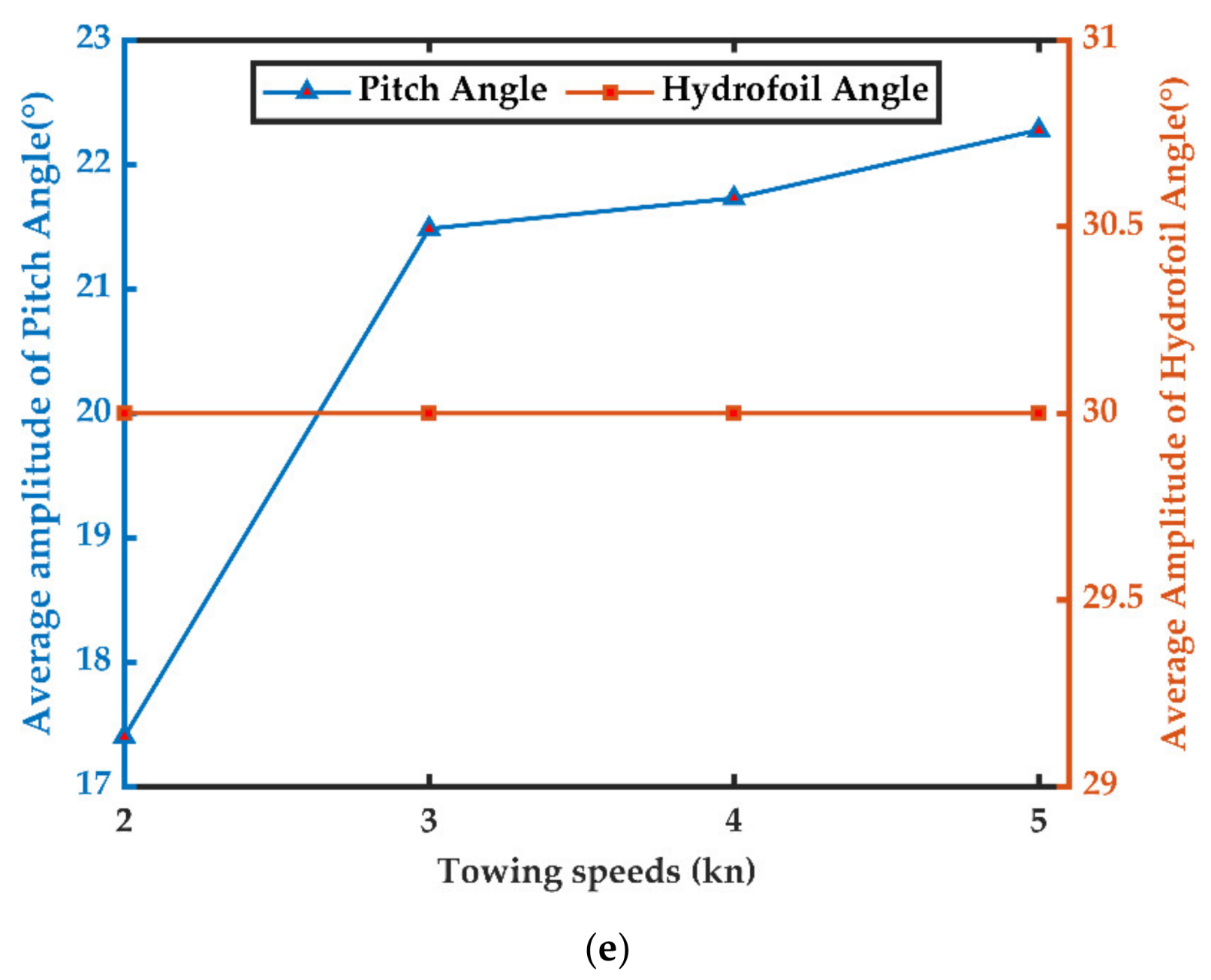
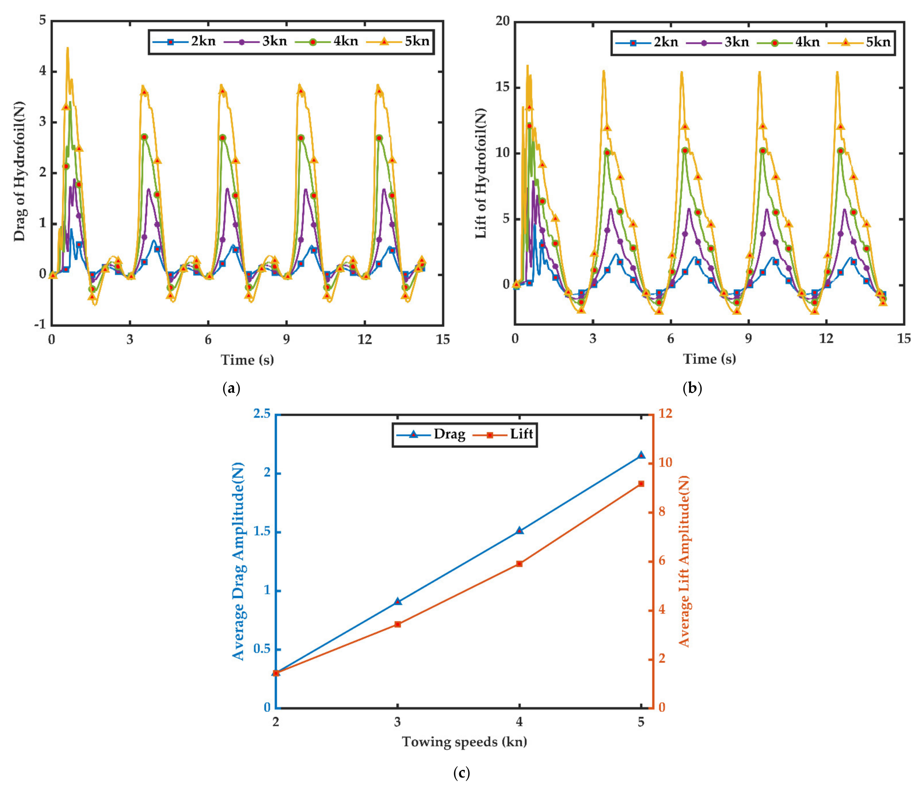
4.2. The Hydrofoil of the Tetherd Underwater Robot

Figure 11a,c present the time histories of the hydrofoil’s drag and the average amplitude of drag at different towing speeds. The hydrofoil’s drag presents a growing linear trend with increases in the towing speed. It fluctuates between −0.60 and 4.49 N when towing speed increases to 5 knots. There is a significant increase in the average amplitude of the hydrofoil’s drag, with the value of 609.71% at 5 knots, compared to the average amplitude of hydrofoil’s drag at 2 knots. It is indicated that the hydrofoil’s drag is greatly influenced by the towing speed. The time history of the hydrofoil’s lift at different towing speeds is presented in Figure 11b. With the increase in the towing speed, the hydrofoil’s lift increases, which shows a linear trend. It oscillates between −2.08 and 16.26 N when towing speed increases to 5 knots. Figure 11c shows that the average amplitude of the hydrofoil’s lift increases to 137.81% at 3 knots, 309.21% at 4 knots, and 535.11% at 5 knots, contrasting to the hydrofoil’s drag at 2 knots. The fluctuation of the hydrofoil’s lift is uniform with the heave of the tethered underwater robot, which demonstrates that the motion of tethered underwater robots is mainly influenced by the control effect of the hydrofoil.

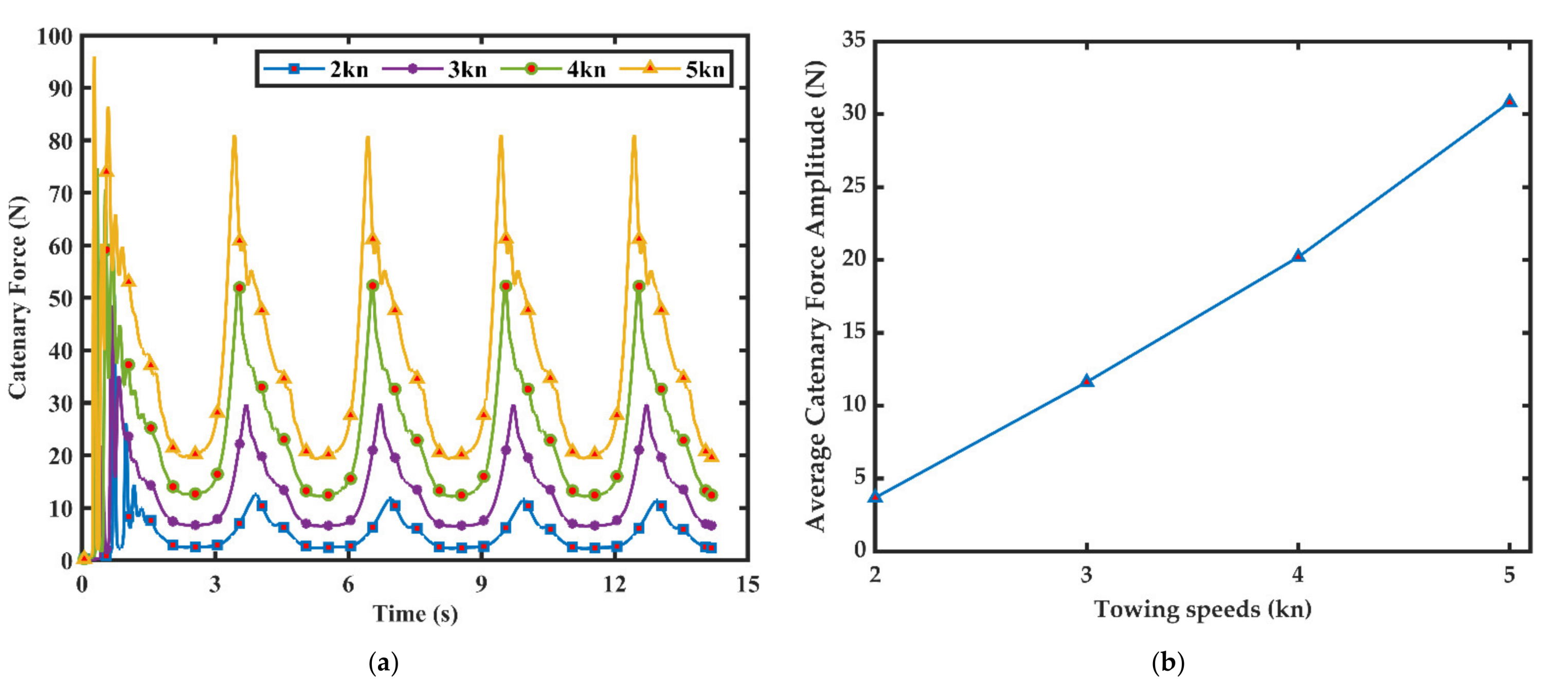
4.3. The Cable of the Tetherd Underwater Robot

The time history of cable force at different towing speeds is shown in Figure 12a, and the cable force fluctuates with the period of 3 s. It can be found that the force of the cable is almost consistent with the fluid resistance after the flow field becomes steady. The cable force is decomposed into gravity and tension, while the mass of the cable is so small that gravity can be ignored. The tension of cable and fluid resistance of the tethered underwater robots becomes an interaction force, which explains the same force. The average amplitude of cable force amplitude is presented in Figure 12b. The increment of average cable force amplitude ranges between 233.44% and 288.04% when the towing speed increases with the interval of 1 knot, which shows that the cable force is greatly influenced by the towing speed.

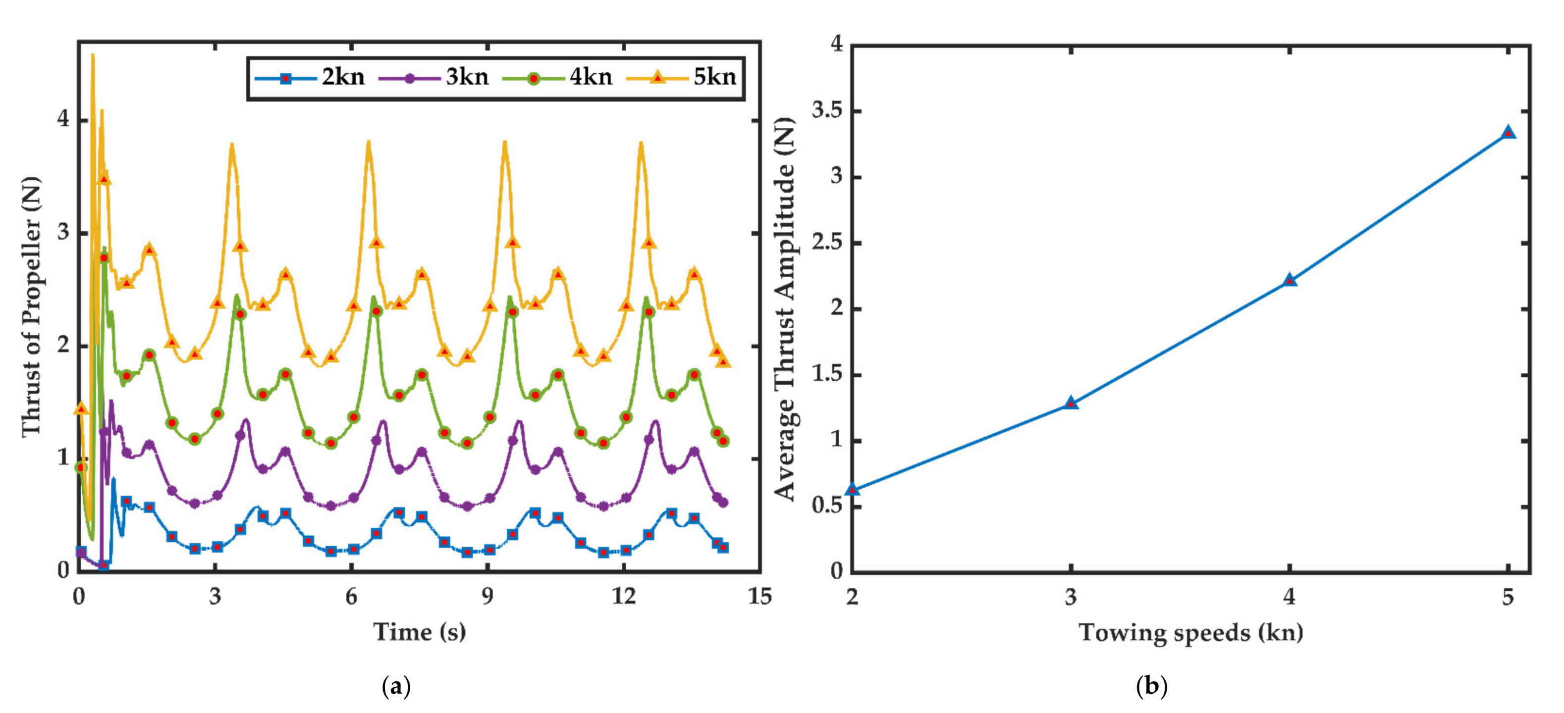
4.4. The Ducted Propeller of the Tetherd Underwater Robot

Figure 13a presents the time history of the thrust of propellers at different towing speeds. The direction of thrust issued the ducted propellers is in contrast with the direction of the tethered underwater robot’s motion when the towing speed increase to 2 knots. Figure 13b shows that the average thrust amplitude of the ducted propeller increases by 33.69% at 3 knots, 61.66% at 4 knots, and 81.31% at 5 knots, compared to the average thrust of the ducted propeller at 2 knots. The thrust of the ducted propeller fluctuates with the period of 3 s, and the fluctuation of thrust is related to the pitch of the tethered underwater robot. The tethered underwater robot’s pitch shows a sine regularity under the control of the hydrofoil, which influences the inflow of ducted propellers. The increases in thrust are also attributed to the advanced velocity’s increase when the towing speed increases. From the above discussion, one can find that the control effect of the ducted propeller is influenced by the tethered underwater robot’s posture and towing speed.

5. Conclusions

A three-dimensional integrated tethered underwater robot with ducted propellers and hydrofoils is constructed to investigate the tethered underwater robot’s hydrodynamic performance at different towing speeds. To clarify the hydrodynamic performance of the tethered underwater robot with control equipment from integrity, the novel numerical method mixing overlapping grid, sliding mesh, the cable coupling model, and the six-DOF model is used, which can simulate the motion of the tethered underwater robot and the rotation of hydrofoils and the ducted propellers. The reliability of the numerical method of dealing with complex motion is validated by the experimental data.

The numerical results show that the control effect and hydrodynamic performance of the tethered underwater robot are greatly influenced by the towing speeds. With the increase in towing speeds, the amplitude of heave increases under the manipulation of control equipment. The tethered underwater robot trajectory is consistent with the swing of hydrofoils, which shows the effectiveness of control with hydrofoils. The cable force is consistent with the tethered underwater robot’s fluid resistance after the flow field becomes steady. The thrust of ducted propellers is related to the towing speed and the tethered underwater robot’s pitch. With a certain propeller speed and tethered underwater robot pitch angle, the bigger the towing speed, the bigger the thrust of the ducted propeller.

References

1. Li, X.F.Y.L.; Wang, H.W. Modeling and Dynamics Analysis of Work-Class ROV Propeller; Transaction of Beijing Institute of Technology: Beijing, China, 2018; Volume 8, pp. 612–618. [Google Scholar]
2. Ablow, C.; Schechter, S. Numerical simulation of undersea cable dynamics. Ocean Eng. 1983, 10, 443–457. [Google Scholar] [CrossRef]
3. Chai, Y.T.; Varyani, K.S.; Barltrop, N.D.P. Three-dimensional Lump-Mass formulation of a catenary riser with bending, torsion and irregular seabed interaction effect. Ocean Eng. 2002, 29, 1503–1525. [Google Scholar] [CrossRef]
4. Walton, T.S.; Polachek, H. Calculation of Transient Motion of Submerged Cables. Math. Comput. 1960, 14, 27–46. [Google Scholar] [CrossRef]
5. Luis Álvaro, R.; Armesto, J.A.; Guanche, R.; Barrera, C.; Vidal, C. Simulation of Marine Towing Cable Dynamics Using a Finite Elements Method. J. Mar. Sci. Eng. 2020, 8, 140. [Google Scholar] [CrossRef] [Green Version]
6. Laranjeira, M.; Dune, C.; Hugel, V. Catenary-based visual servoing for tether shape control between underwater vehicles. Ocean Eng. 2020, 200, 107018. [Google Scholar] [CrossRef]
7. Palm, J.; Eskilsson, C. Influence of Bending Stiffness on Snap Loads in Marine Cables: A Study Using a High-Order Discontinuous Galerkin Method. J. Mar. Sci. Eng. 2020, 8, 795. [Google Scholar] [CrossRef]
8. Li, Q.; Cao, Y.; Li, B.; Ingram, D.M.; Kiprakis, A. Numerical Modelling and Experimental Testing of the Hydrody-namic Characteristics for an Open-Frame Remotely Operated Vehicle. J. Mar. Sci. Eng. 2020, 8, 688. [Google Scholar] [CrossRef]
9. Wu, J.; Chwang, A.T. A hydrodynamic model of a two-part underwater towed system. Ocean Eng. 2000, 27, 455–472. [Google Scholar] [CrossRef]
10. Wu, J.; Chen, D. Trajectory Following of a Tethered Underwater Robot with Multiple Control Techniques. J. Offshore Mech. Arct. Eng. 2019, 141, 051104. [Google Scholar] [CrossRef]
11. Wu, J.; Ye, J.; Yang, C.; Chen, Y.; Tian, H.; Xiong, X. Experimental study on a controllable underwater towed system. Ocean Eng. 2005, 32, 1803–1817. [Google Scholar] [CrossRef]
12. Park, H.I.; Jung, D.H.; Koterayama, W. A numerical and experimental study on dynamics of a towed low tension cable. Appl. Ocean Res. 2003, 25, 289–299. [Google Scholar] [CrossRef]
13. Bagheri, A.; Karimi, T.; Amanifard, N. Tracking performance control of a cable communicated underwater vehicle using adaptive neural network controllers. Appl. Soft Comput. 2010, 10, 908–918. [Google Scholar] [CrossRef]
14. Guerrero, J.; Torres, J.; Creuze, V.; Chemori, A.; Campos, E. Saturation based nonlinear PID control for underwater vehicles: Design, stability analysis and experiments. Mechatronics 2019, 61, 96–105. [Google Scholar] [CrossRef] [Green Version]
15. Zhang, G.; Huang, H.; Qin, H.; Wan, L.; Li, Y.; Cao, J.; Su, Y. A novel adaptive second order sliding mode path following control for a portable AUV. Ocean Eng. 2018, 151, 82–92. [Google Scholar] [CrossRef]
16. Chen, D.J.; Wu, J.M. Control simulation and hydrodynamics analysis of a tethered underwater robot. J. Ship Mech. 2020, 24, 170–178. [Google Scholar]
17. Zhou, H.; Wei, Z.; Zeng, Z.; Yu, C.; Yao, B.; Lian, L. Adaptive robust sliding mode control of autonomous underwater glider with input constraints for persistent virtual mooring. Appl. Ocean Res. 2020, 95, 102027. [Google Scholar] [CrossRef]
18. Yu, L.; Meng, Q.; Zhang, H. 3-Dimensional Modeling and Attitude Control of Multi-Joint Autonomous Underwater Vehicles. J. Mar. Sci. Eng. 2021, 9, 307. [Google Scholar] [CrossRef]
19. Zhou, B.; Zhao, M. Numerical simulation of thruster-thruster interaction for ROV with vector layout propulsion system. Ocean Eng. 2020, 210, 107542. [Google Scholar] [CrossRef]
20. Vu, M.T.; Choi, H.; Kang, J.; Ji, D.-H.; Jeong, S.-K. A study on hovering motion of the underwater vehicle with umbilical cable. Ocean Eng. 2017, 135, 137–157. [Google Scholar] [CrossRef]
21. Fang, M.-C.; Hou, C.-S.; Luo, J.-H. On the motions of the underwater remotely operated vehicle with the umbilical cable effect. Ocean Eng. 2007, 34, 1275–1289. [Google Scholar] [CrossRef]
22. Wu, J.M.; Yu, M.; Zhu, L.L. A hydrodynamic model for a tethered underwater robot and dynamic analysis of the robot in turning motion. J. Ship Mech. 2011, 15, 827–836. [Google Scholar]
23. Wu, J.M.; Ye, Z.J.; Jin, X.D.; Zhang, C.W.; Xu, Y. Analysis of thrust characteristics of ducted propeller in underwater vehicle with yawing motion. J. South China Univ. Technol. 2015, 43, 141–148. [Google Scholar]
24. Tsan-Hsing Shih, W.W.L.; Aamir, S.Z.Y.; Zhu, J. A new k-ε eddy viscosity model for high reynolds number turbulent flows. Comput. Fluids 1995, 24, 227–238. [Google Scholar] [CrossRef]
25. Gertler, M.; Hagen, G.R. Standard Equations of Motion for Submarine Simulation; Defense Technical Information Center (DTIC): Fort Belvoir, VA, USA, 1967. [Google Scholar]
26. Hongwei, Z.; Shuxin, W.; Wei, H.; Manli, H. Research on 3D modeling of propeller. Mach. Tool Hydraul. 2006, 60, 3. [Google Scholar]
Figure 1. The cable and its force.
Jmse 09 00561 g001
Figure 2. The diagram of the overlapping grid and the procedure of numerical simulation applied the overlapping grid: (a) the cells of the tethered underwater robot’s overlapping grid; (b) the procedure of numerical calculation.
Jmse 09 00561 g002
Figure 3. The profile of the tethered underwater robot: (a) the front view of the tethered underwater robot and rotation angle of hydrofoils; (b) the top view of the tethered underwater robot; (c) the back view of the tethered underwater robot and direction of rotation; (d) the isometric view of the tethered underwater robot.
Jmse 09 00561 g003aJmse 09 00561 g003b
Figure 4. Computational domain of the underwater robot: (a) Domain I: propeller and hydrofoil; (b) Domain II: underwater robot; (c) distribution of the computational domain.
Jmse 09 00561 g004
Figure 5. The cutaway view of computational domain mesh: (a) the left view of the computational domain; (b) the front view of the computational domain.
Jmse 09 00561 g005
Figure 6. The comparison of submerged depth and pitch angle between experiment and numerical simulation. (a) The tethered underwater robot’s submerged depth. (b) The tethered underwater robot’s pitch angle.
Jmse 09 00561 g006
Figure 7. Time history of the trajectory of the tethered underwater robot at different towing speeds: (a) the tethered underwater robot’s surge; (b) the tethered underwater robot’s heave; (c) the average amplitude of surge and heave; (d) the trajectory of the tethered underwater robot.
Jmse 09 00561 g007
Figure 8. Time history of the velocity of the tethered underwater robot at different towing speeds: (a) the surge velocity of the tethered underwater robot; (b) the heave velocity of the tethered underwater robot; (c) the average velocity amplitude of surge and heave.
Jmse 09 00561 g008
Figure 9. The time history of the pitch velocity, acceleration and angle of the tethered underwater robot at different towing speeds: (a) the pitch velocity of the tethered underwater robot; (b) the pitch acceleration of the tethered underwater robot; (c) the pitch angle of the tethered underwater robot; (d) the average amplitude of the tethered underwater robot’s pitch velocity and acceleration; (e) the average amplitude of the tethered underwater robot’s pitch angle and the average amplitude hydrofoil’s angle.
Jmse 09 00561 g009aJmse 09 00561 g009b
Figure 10. The time history of the fluid resistance and moment of the tethered underwater robot at different towing speeds: (a) the fluid resistance of the tethered underwater robot; (b) the fluid resistance moment of the tethered underwater robot; (c) the average amplitude of fluid resistance amplitude and fluid resistance moment.
Jmse 09 00561 g010aJmse 09 00561 g010b
Figure 11. Time history of the drag and lift of the hydrofoil at different towing speeds: (a) drag of the hydrofoil; (b) lift of the hydrofoil; (c) average drag and lift amplitude.
Jmse 09 00561 g011
Figure 12. Time history of the of cable force at different towing speeds: (a) cable force; (b) average cable force amplitude.
Jmse 09 00561 g012
Figure 13. Time history of the thrust of the ducted propeller at different towing speeds: (a) thrust of the ducted propeller; (b) average thrust amplitude.
Jmse 09 00561 g013