Higher-Harmonic Response of a Slender Monopile to Fully Nonlinear Focused Wave Groups

Abstract

The “ringing” response of a monopile foundation to focused wave groups was investigated in this study. Such responses are of practical interest in the context of offshore wind turbine foundations. Moderately steep transient focused wave groups were generated in a novel numerical wave tank, based on the high-order spectral method, which was verified and in good agreement with published laboratory data. The monopile was simplified into a slender linear elastic cantilever beam to measure the severity of the structural response. The resonant behavior was excited at the triple-wave frequency of the wave loads. The influence of the damping ratio on the ringing response was considered. Different incident wave models and hydrodynamic models were used to predict the wave loads and induced responses over different wave steepness. The wavelet transform was successfully applied to reveal the local characteristics of the wave loads and ringing response.

1. Introduction

The rapid expansion of the offshore wind industry has aroused great interest in the behavior of monopile foundations. It is necessary to develop suitable and efficient tools for assessing their reliability and survivability when exposed to steep transient water waves. The peak frequencies of the most common sea states are lower than the first natural frequency of the structure. However, Ridder et al. [1] found that waves with higher harmonics close to the first natural frequency of the structure can still induce a resonant response. This phenomenon, called “ringing,” typically occurs when the natural frequency of the monopile is approximately three to five times the wave frequency. The ringing phenomenon was discussed intensively in the 1990s for deep-water tension leg platforms (TLPs). For instance, as reported for model tests by Natvig and Teigen [2], the third-order forcing caused a resonant response for TLP structures. Bredmose et al. [3] investigated the hydro-elastic problem of structural response to fully nonlinear regular wave forcing of a cantilever beam. However, as Atkins et al. [4] mentioned, large transient wave groups are more likely to induce the ringing phenomenon instead of a regular wave train. The response is characterized by a rapid onset of vibration in the natural mode after the passage of a large wave, and it damps out eventually. In this study, an attempt was made to interpret a more realistic and complex case of large focused wave groups, which can be essential in the quest for structural strength design.

In recent decades, considerable efforts have been made to actualize numerical simulations of wave–structure interactions. Analytical theories based on conventional perturbation theory, such as linear and second-order wave diffraction–radiation models, cannot calculate well the higher-harmonic wave loads leading to ringing. These theories, formally assuming a small steepness of the incident wave, are only valid for a moderate wave amplitude. Therefore, to ensure survival in a hostile environment, Rainey [5,6] developed a fully nonlinear load model for slender structures. The alternative model was derived from energy considerations instead of the conventional perturbation method. This model is regarded as an extended version of the Morison equation, making it possible to compute the loads based only on the incident wave, overlooking the effect of the disturbed waves. Compared with the standard Morison equation, the extension contains two parts: one for the axial divergence of the flow (see also a previous report [7]) and the other for a point force at the intersection with the free surface. The principal advantage of Rainey’s model is that it can be employed in extreme wave cases.

Even if the presence of the structure within the wave field is neglected, modeling of an extreme wave event is still a complex problem. The complexity arises from its highly nonlinear and transient properties within an irregular and multifrequency sea state. In this study, the NewWave model proposed by Tromans et al. [8], where many wave components in a spectrum focus simultaneously at a position, was adopted to model the average shape for an extreme wave profile. Numerical wave tanks (NWTs), which are able to accurately reproduce realistic wave fields, have received considerable attention and have been widely applied in many ocean engineering projects. Many successful mathematical models found in several previous work are developed based on various numerical schemes, using the fully nonlinear potential flow model REEF3D::FNPF [9], the operational model SWASH [10], the pseudo-spectral model HOST-wm3 [11], and the CFD NWT designed in OpenFOAM [12]. To evaluate the capacity of different models, a cross-validation of the surface dynamics among the models OpenFOAM, SWASH, and HOST-wm3 has been performed in [13]. In this paper, an extreme wave was generated in a novel numerical wave tank, based on the high-order-spectral (HOS) method [14,15] (called “HOS-NWT” hereinafter). Owing to the fast Fourier transform (FFT) solution, it exhibits a high level of efficiency properties. Ducrozet et al. [11] developed an NWT (HOST-wm3) whose wavemaker boundary condition was treated by prescribing the wavemaker motion at the upstream boundary and expanded up to third order by the perturbation method. However, with highly nonlinear phenomena, such as extreme focused wave groups, etc., sawtooth instabilities appear in the wavemaker solution, and no satisfactory scheme has been obtained to solve this problem [11]. In this study, to modify the wavemaker solution, following Ning et al. [16], the fluid motion was generated by feeding wave properties from the tank floor to the instantaneous free surface according to a chosen wave theory at the inflow boundary. To resemble the input motion of the fluid particle as accurately as possible, the second-order Stokes theory [17] for irregular waves was chosen in this study. Numerical simulations of focused wave groups were performed, and the simulated results were compared with the experimental data and theoretical input waves.

The aim of this study was to provide an efficient, simple, but accurate model for predictions of higher-harmonic wave loads and the induced ringing response. Under the assumption of a small ratio of diameter to wave length, a numerical model is presented, consisting of the spectral methods for the incident waves, Rainey’s model for nonlinear wave loads, and the linear Euler–Bernoulli beam equation for the ringing response. Following the introduction, the remainder of this article is organized as follows. In Section 2, the problem definition and the mathematical formulation are introduced. The convergence study and validation of the proposed model are presented in Section 3. Subsequently, the effects of different damping ratios, wave steepness, incident wave models, and hydrodynamic models on wave loadings and induced responses are described in Section 4. Moreover, wavelet-based analyses conducted to study the local characteristics of the wave loads and the related ringing response are discussed. Finally, concluding remarks are presented in Section 5.

2. Mathematical Formulation

In this section, the method to obtain a fully nonlinear incident wave solution by spectral wave representations based on the potential flow theory and the way to solve the hydro-elastic model for monopiles are described.

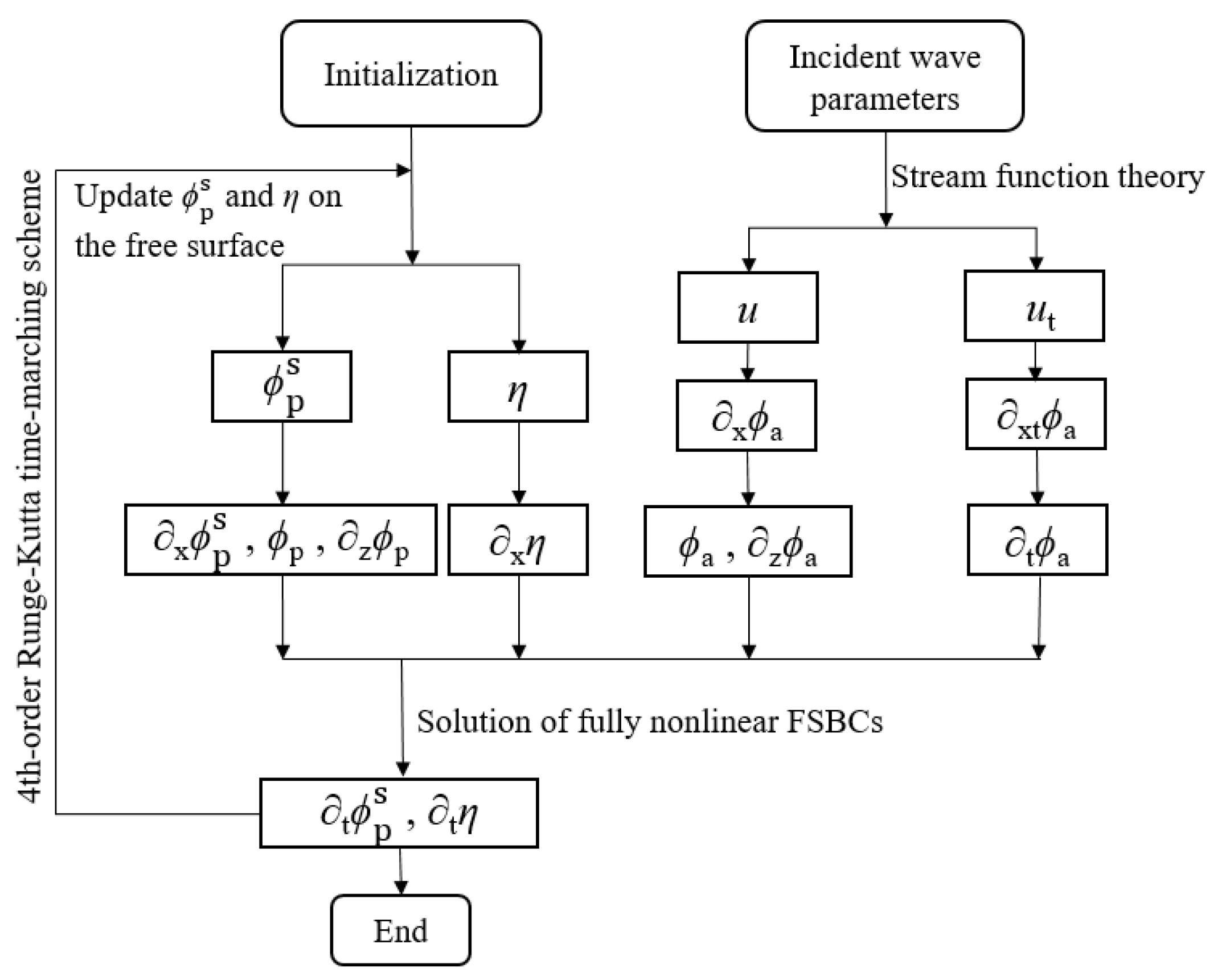
2.1. Incident Wave Modeling: Spectral Solution Representations

A Cartesian coordinate system Oxyz is defined to simulate nonlinear wave events, with the origin O in the plane of the undisturbed free surface, x measuring in the direction of incident wave propagation, and z measuring upward from the still-water level, as indicated in Figure 1. The fluid is assumed to be incompressible and inviscid, together with the assumption of irrotational flow. The velocity potential ϕ(x,z,t) can therefore be introduced to describe the fluid motion, which satisfies the Laplace equation in the fluid domain:

$$\Delta \varphi (x,z,t)=0.$$

(1)

On the instantaneous free surface, both the fully nonlinear kinematic and dynamic boundary conditions, derived from the material derivatives and the Bernoulli equation, respectively, must always be fulfilled:

$${\partial }_{\mathrm{t}}\eta ={\partial }_{\mathrm{z}}\varphi -{\partial }_{\mathrm{x}}\varphi {\partial }_{\mathrm{x}}\eta ,\hspace{1em}\mathrm{on} z=\eta ,$$

(2)

$${\partial }_{\mathrm{t}}\varphi =-g\eta -\frac{1}{2}\left({\left|{\partial }_{\mathrm{x}}\varphi \right|}^2+{\left|{\partial }_{\mathrm{z}}\varphi \right|}^2\right),\hspace{1em}\mathrm{on} z=\eta ,$$

(3)

where g is the acceleration caused by gravity, and η denotes the free-surface elevation above the still-water level. The kinematic boundary condition on the seabed is:

$${\partial }_{\mathrm{n}}\varphi =0,\hspace{1em}\mathrm{on} z=-d,$$

(4)

where d denotes the finite water depth. The boundary-value problem can be solved using spectral methods by means of a set of basis functions. The free-surface elevation η(x,t) and the velocity potential ϕ(x,z,t) can be decomposed as follows:

$$\eta (x,t)={\displaystyle \sum _{i=0}^N{A}_{\mathrm{i}}^{\mathsf{\eta }}}(t){\psi }_{\mathrm{i}}(x),$$

(5)

$$\varphi (x,z,t)={\displaystyle \sum _{i=0}^N{A}_{\mathrm{i}}^{\varphi }}(t)\frac{\cosh \left(k_{\mathrm{i}}(z+d)\right)}{\cosh \left(k_{\mathrm{i}}d\right)}{\psi }_{\mathrm{i}}(x),$$

(6)

where k_i are the basis wave numbers, and ψ_i(x) are the horizontal basis functions (sine and cosine functions or their complex exponential equivalents, satisfying the Laplace equation and the seabed boundary condition automatically). Here, N is the number of Fourier components, and $A_{\mathrm{i}}^{\mathsf{\eta }}$(t) and $A_{\mathrm{i}}^{\varphi }$(t) are the modal amplitudes determined by the free-surface boundary conditions (FSBCs) in Equations (2) and (3). Stream function wave theory [18] is adopted for regular waves, and the HOS-NWT for focused wave groups.

2.1.1. Stream Function Theory for Regular Waves

For the progressive regular wave, Rienecker and Fenton [18] provided a fully nonlinear solution. The stream function Ψ is decomposed using the basis functions as follows:

$$\Psi (x,z,t)=B_{0}z+{\displaystyle \sum _{j=1}^N{B}_j}\frac{\sinh jkz}{\cosh jkd}\cos jk(x-ct),$$

(7)

where k is the wave number, and c is the phase velocity of each compositing wave. These amplitudes, B_j, are solved numerically from the systems of nonlinear equations using Newton’s method. More information can be found in the report by Rienecker and Fenton [18].

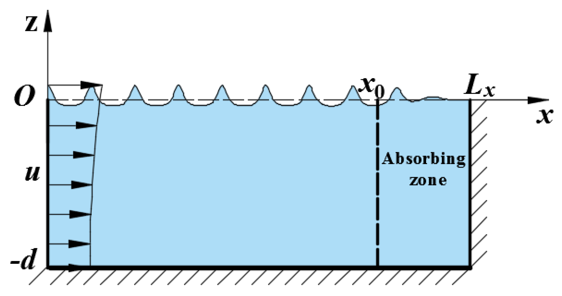
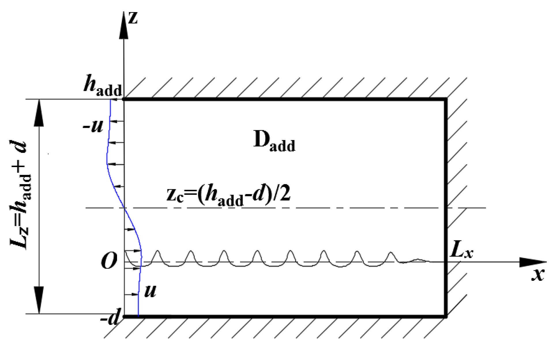
2.1.2. High-Order Spectral Numerical Wave Tank for Focused Wave Groups

For irregular waves, a two-dimensional wave tank is established with horizontal dimension L_x and finite depth d, as shown in Figure 2. An absorbing zone is included near the end wall x = L_x through a local modification of the free-surface dynamic boundary condition, which is described using a local modification of pressure at the free surface:

$$p_{\mathrm{a}}=\rho \nu (x){\partial }_{\mathrm{t}}\eta ,$$

(8)

where ρ is the fluid density, and the function ν(x) is nonzero, where an absorption zone is required.

$$\nu \left(x\right)=\{\begin{array}{ll}0& x<x_0\\ \alpha {\mu }^2\left(3-2\mu \right)& x\ge x_0\end{array},$$

(9)

where x₀ is the starting point of the absorbing zone, μ = (x − x₀)/(L_x − x₀), and α is the strength of the absorbing zone (see previous research [19,20] for more details). Then, the free-surface boundary condition in Equation (3) is rewritten as follows:

$${\partial }_{\mathrm{t}}\varphi =-g\eta -\frac{1}{2}\left({\left|{\partial }_{\mathrm{x}}\varphi \right|}^2+{\left|{\partial }_{\mathrm{z}}\varphi \right|}^2\right)-\nu {\partial }_{\mathrm{t}}\eta ,\hspace{1em}\mathrm{on} z=\eta .$$

(10)

At the inflow boundary, a theoretical particle velocity profile is prescribed from the bottom to the free surface:

$${\partial }_{\mathrm{x}}\varphi =u(z), \mathrm{on} x = 0,$$

(11)

where u is the horizontal velocity of the underlying water particle kinematics. In addition, a nonflow condition is used on other boundaries:

$$\{\begin{array}{c}{\partial }_{\mathrm{n}}\varphi =0,\hspace{1em}\mathrm{on} x=L_{\mathrm{x}}\\ {\partial }_{\mathrm{n}}\varphi =0,\hspace{1em}\mathrm{on} z=-d\end{array}.$$

(12)

Owing to the stochastic nature of the focused wave groups, according to the NewWave model, the amplitude spectrum of discrete wave components can be determined by a practical spectrum as:

$$A_{\mathrm{i}}=A\frac{S(f_{\mathrm{i}})\Delta f}{{\displaystyle \sum _{i=1}^{N}S}(f_{\mathrm{i}})\Delta f},$$

(13)

where A is the input linear sum of the component wave amplitudes, which occurs at the focus location and time, N is the total number of discrete wave components, A_i is the amplitude of each wave component, f is the frequency (inversion of wave period), and S(f) denotes the corresponding wave spectrum. The energy spectrum proposed by the Joint North Sea Wave Project (JONSWAP) [21] with a peak enhancement factor of γ = 3.30 is used to obtain the underlying wave components. Then, the second-order Stokes theory is used to specify the corresponding velocity:

$$u=u^{\left(1\right)}+u^{\left(2\right)},$$

(14)

where the linear velocity u⁽¹⁾ and the second-order velocity u⁽²⁾ can be referred to previous work [16] and thus are not elaborated here.

The computation domain of the NWT is nonperiodic owing to the presence of the wavemaker. Such cases lead to the idea of the potential decomposition concept [22], where the original potential ϕ is separated into two components:

$$\varphi ={\varphi }_{\mathrm{p}}+{\varphi }_{\mathrm{a}},$$

(15)

where ϕ_p is the periodic potential derived by imposing reflecting lateral boundary conditions, and ϕ_a is the additional potential accounting for the wavemaker boundary condition, describing the evanescent modes that decay exponentially away from the boundary. The boundary conditions of ϕ_p can be written as:

$$\{\begin{array}{c}{\partial }_{\mathrm{n}}{\varphi }_{\mathrm{p}}=0,\hspace{1em}\mathrm{on} x=0\\ {\partial }_{\mathrm{n}}{\varphi }_{\mathrm{p}}=0,\hspace{1em}\mathrm{on} x=L_{\mathrm{x}}\\ {\partial }_{\mathrm{n}}{\varphi }_{\mathrm{p}}=0,\hspace{1em}\mathrm{on} z=-d\end{array}.$$

(16)

The additional potential ϕ_a satisfies the wavemaker condition at the left end of the tank:

$${\partial }_{\mathrm{x}}{\varphi }_{\mathrm{a}}=u(z),\hspace{1em}\mathrm{on} x=0.$$

(17)

A nonflow condition is used on other boundaries:

$$\{\begin{array}{l}{\partial }_{\mathrm{n}}{\varphi }_{\mathrm{a}}=0,\hspace{1em}\mathrm{on} x=L_x\\ {\partial }_{\mathrm{n}}{\varphi }_{\mathrm{a}}=0,\hspace{1em}\mathrm{on} z=-d\end{array}.$$

(18)

To formulate the FSBCs with dependence on the horizontal coordinate only following Zakharov’s method [23], the periodic surface potential on the free surface is partially defined as:

$${\varphi }_{\mathrm{p}}^{\mathrm{s}}(x,t)={\varphi }_{\mathrm{p}}(x,z=\eta ,t).$$

(19)

Introducing the derivatives that stem from this definition:

$${\partial }_{\mathrm{x}}{\varphi }_{\mathrm{p}}={\partial }_{\mathrm{x}}{\varphi }_{\mathrm{p}}^{\mathrm{s}}-{\partial }_{\mathrm{z}}{\varphi }_{\mathrm{p}}\hspace{0.17em}{\partial }_{\mathrm{x}}\eta ,$$

(20)

$${\partial }_{\mathrm{t}}{\varphi }_{\mathrm{p}}={\partial }_{\mathrm{t}}{\varphi }_{\mathrm{p}}^{\mathrm{s}}-{\partial }_{\mathrm{z}}{\varphi }_{\mathrm{p}}\hspace{0.17em}{\partial }_{\mathrm{t}}\eta .$$

(21)

Using the separated potential representation Equation (15), the fully nonlinear free-surface conditions can be expressed as:

$${\partial }_{\mathrm{t}}\eta =\left[1+{\left({\partial }_{\mathrm{x}}\eta \right)}^2\right]W+{\partial }_{\mathrm{z}}{\varphi }_{\mathrm{a}}-\left({\partial }_{\mathrm{x}}{\varphi }_{\mathrm{p}}^{\mathrm{s}}+{\partial }_{\mathrm{x}}{\varphi }_{\mathrm{a}}\right){\partial }_{\mathrm{x}}\eta ,\hspace{1em}\mathrm{on} z=\eta ,$$

(22)

$$\begin{array}{l}{\partial }_{\mathrm{t}}{\varphi }_{\mathrm{p}}^{\mathrm{s}}=-g\eta +\frac{1}{2}\left[1+{\left({\partial }_{\mathrm{x}}\eta \right)}^2\right]W^2-\frac{1}{2}{\left({\partial }_{\mathrm{z}}{\varphi }_{\mathrm{a}}\right)}^2\\ \begin{array}{ccc}& & \end{array}-\frac{1}{2}{\left({\partial }_{\mathrm{x}}{\varphi }_{\mathrm{p}}^{\mathrm{s}}+{\partial }_{\mathrm{x}}{\varphi }_{\mathrm{a}}\right)}^2-{\partial }_{\mathrm{t}}{\varphi }_{\mathrm{a}}-\nu {\partial }_{\mathrm{t}}\eta ,\hspace{1em}\mathrm{on} z=\eta \end{array},$$

(23)

where W = ∂_zϕ_p (x, z = η, t), which can be computed following the original HOS method [14,15] as follows:

$$\{\begin{array}{c}W={\displaystyle \sum _{m=1}^M}{W}^{(\mathrm{m})},\\ W^{\left(\mathrm{m}\right)}={\displaystyle \sum _{j=0}^{m-1}}\frac{{\eta }^{\mathrm{j}}}{j!}{\partial }_{\mathrm{z}}^{\mathrm{j}+1}{\varphi }_{\mathrm{p}}^{(\mathrm{m}-\mathrm{j})}(x,0,t),\hspace{1em}m=1,2,\dots ,M\end{array},$$

(24)

where M is the order of nonlinearity, which is chosen as M = 7, whereas the value of N is selected specifically for each simulation. Because ϕ_p has zero flux through the left, right, and bottom boundaries, the spectral expansions chosen for it are:

$$\{\begin{array}{c}{\varphi }_{\mathrm{p}}(x,z,t)={\displaystyle \sum _{m=1}^M}{\varphi }_{\mathrm{p}}^{\left(\mathrm{m}\right)}(x,z,t)\\ {\varphi }_{\mathrm{p}}^{\left(\mathrm{m}\right)}(x,z,t)={\displaystyle \sum _{n=0}^{N_{\mathrm{x}}}}{A}_{\mathrm{n}}^{\left(\mathrm{m}\right)}(t)\frac{\cosh \left[k_{\mathrm{n}}(z+d)\right]}{\cosh k_{\mathrm{n}}d}\cos k_{\mathrm{n}}x\end{array},$$

(25)

where $A_{\mathrm{n}}^{\left(\mathrm{m}\right)}$(t) is the modal amplitudes, the natural eigenmodes of the wave tank are k_n = nπ/L_x, and N_x is the number of wave modes that are considered. Furthermore, each ${\varphi }_{\mathrm{p}}^{\left(\mathrm{m}\right)}$ is expanded in a Taylor series around z = 0. The following scheme is arranged according to the order m:

$$\{\begin{array}{c}{\varphi }_{\mathrm{p}}^{(1)}(x,0,t)={\varphi }_{\mathrm{p}}^{\mathrm{s}}(x,t),\hspace{1em}for m = 1\\ {\varphi }_{\mathrm{p}}^{\left(\mathrm{m}\right)}(x,0,t)=-{\displaystyle \sum _{k=1}^{m-1}}\frac{{\eta }^{\mathrm{k}}}{k!}\frac{{\partial }^{\mathrm{k}}{\varphi }_{\mathrm{p}}^{(\mathrm{m}-\mathrm{k})}}{\partial z^{\mathrm{k}}}(x,0,t),\hspace{1em}for m > 1\end{array}.$$

(26)

Following Bonnefoy et al. [19], ϕ_a is solved in a new extended domain of computation, as shown in Figure 3. This new domain is chosen to have the ability of a fully spectral formulation of the additional problem, which can be solved conveniently by using the FFT. The total height of the extended domain is L_z = h_add + d, and the horizontal velocity along the input boundary is antisymmetric above the central line z_c = (h_add − d)/2. The h_add is selected as 3d following Bonnefoy et al. [19] with central line height z_c = d, such that the central line z_c is higher than the maximum wave height. Another issue worth noting is that Bonnefoy et al. [19] specified the motion of the wave generator from the bottom of the tank to the static water level. Instead, a more reasonable one is proposed for a steep nonlinear wave to feed the input wave properties from the bottom to the free surface. The third-order polynomial function from z = η(t) to z = h_add − d − η(t) is chosen as a matching curve to close smoothly the domain D_add, which is defined as:

$$S(z,t)=(z-z_{\mathrm{c}})\left[c_1(t)+c_2(t){(z-z_{\mathrm{c}})}^2\right].$$

(27)

The coefficients considered at an instantaneous time step are given as:

$$\{\begin{array}{c}{c}_1(t)=-[3u(\eta (t),t)+(d-\eta (t))u_{\mathrm{z}}(\eta (t),t)]/[2(d-\eta (t))]\\ c_2(t)=\left[u(\eta (t),t)+(d-\eta (t))u_{\mathrm{z}}(\eta (t),t)\right]/\left[2{(d-\eta (t))}^3\right]\end{array}.$$

(28)

In this extended domain, the additional potential ϕ_a is expanded as:

$${\varphi }_{\mathrm{a}}(x,z,t)={\displaystyle \sum _{n=1}^{N_{\mathrm{z}}}{B}_{\mathrm{n}}}(t)\cos \left[k_{\mathrm{n}}(z+d)\right]\frac{\cosh \left[k_{\mathrm{n}}\left(L_{\mathrm{x}}-x\right)\right]}{\cosh (k_{\mathrm{n}}{L}_{\mathrm{x}})},$$

(29)

where B_n(t) is the modal amplitudes, and k_n = (2n − 1)π/(h_add + d). Subsequently, the additional derivatives ∂_xϕ_a are expanded analytically as:

$${\partial }_{\mathrm{x}}{\varphi }_{\mathrm{a}}(x,z,t)={\displaystyle \sum _{n=1}^{N_{\mathrm{z}}}-k_{\mathrm{n}}{B}_{\mathrm{n}}}(t)\cos \left[k_{\mathrm{n}}(z+d)\right]\frac{\sinh \left[k_{\mathrm{n}}\left(L_{\mathrm{x}}-x\right)\right]}{\cosh (k_{\mathrm{n}}{L}_{\mathrm{x}})}.$$

(30)

Substituting the special derivatives into Equation (17), the time-dependent coefficients B_n(t) are determined through the explicit known u by means of the FFT method. Once the time-dependent coefficients B_n(t) are determined, ϕ_a is solved eventually.

Instead of using backward finite difference to estimate ∂_tϕ_a, the time derivative is directly obtained through the explicit known u_t by means of the same scheme for ϕ_a. According to Equation (17), the time derivatives also satisfy the wavemaker condition:

$${\partial }_{\mathrm{xt}}{\varphi }_{\mathrm{a}}=u_{\mathrm{t}}(z), \mathrm{on} x = 0.$$

(31)

Here, ∂_tϕ_a and ∂_xtϕ_a are expanded as:

$${\partial }_{\mathrm{t}}{\varphi }_{\mathrm{a}}(x,z,t)={\displaystyle \sum _{n=1}^{N_{\mathrm{z}}}{C}_{\mathrm{n}}}(t)\cos \left[k_{\mathrm{n}}(z+d)\right]\frac{\cosh \left[k_{\mathrm{n}}\left(L_{\mathrm{x}}-x\right)\right]}{\cosh (k_{\mathrm{n}}{L}_{\mathrm{x}})},$$

(32)

$${\partial }_{\mathrm{xt}}{\varphi }_{\mathrm{a}}(x,z,t)={\displaystyle \sum _{n=1}^{N_{\mathrm{z}}}-k_{\mathrm{n}}{C}_{\mathrm{n}}}(t)\cos \left[k_{\mathrm{n}}(z+d)\right]\frac{\sinh \left[k_{\mathrm{n}}\left(L_{\mathrm{x}}-x\right)\right]}{\cosh (k_{\mathrm{n}}{L}_{\mathrm{x}})}.$$

(33)

Substituting Equation (33) into Equation (31), the time-dependent coefficients C_n(t) are determined through the explicit known u_t by means of the FFT method. Subsequently, ∂_tϕ_add is solved eventually.

To reduce any impulse-like behavior at the inlet boundary, a cosine ramping function is applied at the start of the computation. The ramping function is given by:

$$R_{\mathrm{m}}\left(t\right)=\{\begin{array}{c}\frac{1}{2}\left(1-\cos \left(\frac{\pi t}{T_{\mathrm{m}}}\right)\right),\hspace{1em}\begin{array}{cc}& \end{array}t\le T_{\mathrm{m}}\\ 1,\hspace{1em}\begin{array}{cc}\begin{array}{ccc}\begin{array}{cc}\begin{array}{cc}& \end{array}& \end{array}& & \end{array}& \end{array}t>T_{\mathrm{m}}\end{array},$$

(34)

where T_m is the ramp time, chosen as 2T, with T the characteristic wave period. To obtain a time-dependent solution, the initial calm water surface condition is applied in the present model as follows:

$${\varphi }_{{}^{\mathrm{p}}}^{\mathrm{s}}=0,\hspace{1em}\eta =0\begin{array}{cc},& \mathrm{at} t=0\end{array}.$$

(35)

The solution algorithm for the HOS-NWT is schematized in Figure 4. It is divided into two main parts. One addresses the solution of the wave generation problem in D_add, and the other addresses the fully nonlinear FSBCs to obtain ${\varphi }_{\mathrm{p}}^{\mathrm{s}}$ (or equivalently ϕ_p) and η. The fully spectral solution scheme (including the wave generation) makes the FFT-based solution scheme, which exhibits great efficiency, possible. The spatial derivatives of the velocity potentials ϕ_p and ϕ_a are straightforwardly reconstructed from semi-analytical basis expressions. Equations (22) and (23) then provide the time derivatives of the unknowns ${\varphi }_{\mathrm{p}}^{\mathrm{s}}$ and η, which are further used in a time-marching fourth-order Runge–Kutta Cash–Karp scheme with an adaptive step size [24].

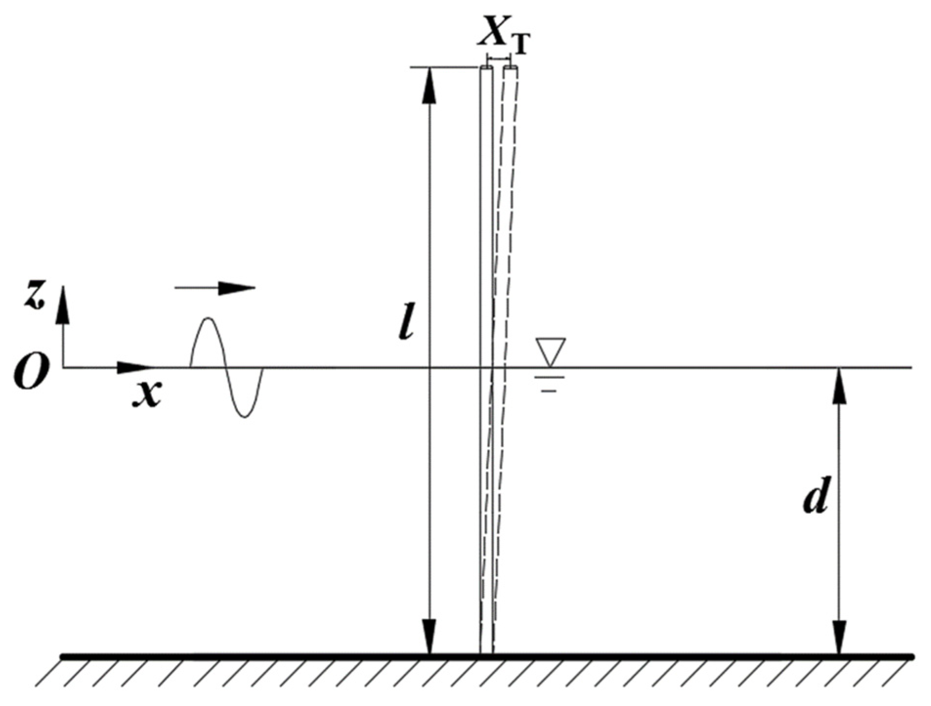
2.2. Hydro-Elastic Model for Monopile

In this section, the complicated hydro-elastic problem for monopile is solved. The monopile has a diameter D, length l, structural mass per unit length $\overline{m}$, and lateral bending stiffness EI, where E is the modulus of elasticity and I is the identical cross-sectional moment of inertia along full length. The bottom of the monopile is embedded in the seabed. The natural frequency of the first mode of vibration is denoted as follows:

$$f_1=\frac{{1.8751}^2}{2\pi }\sqrt{\frac{EI}{\overline{m}{l}^4}}.$$

(36)

Under the assumption of a small ratio of monopile diameter to the wave length, the wave loads can be calculated by neglecting the disturbed waves, using Rainey’s model [5,6]. Instead of a conventional perturbation approach, Rainey’s model was derived from energy considerations, allowing the numerical computation of wave loading induced by regular and irregular waves. The loads per unit length of a monopile can be written as:

$$\begin{array}{l}f(t,z)=\rho A{C}_{\mathrm{m}}(\dot{u}-\ddot{X})+\rho A\dot{u}+\rho A{C}_{\mathrm{m}}{w}_{\mathrm{z}}(u-\dot{X})\\ \begin{array}{cccc}& & & +\frac{1}{2}\rho C_{\mathrm{D}}D(u-\dot{X})|u-\dot{X}|\end{array}\end{array}$$

(37)

where C_m is the added mass coefficient, C_D is the drag coefficient, ρ is the density of water, A = πD²/4 is the structural cross-sectional area, u and w are the horizontal and vertical particle velocity components, respectively, and ($\dot{X}$, $\ddot{X}$) are the structural velocity and acceleration, respectively. Furthermore, $\dot{u}$ is the Lagrangian water particle acceleration ($\dot{u}$ = u_t + uu_x + wu_z for the present 2D flow), and the last inertia term in Equation (37) is the axial divergence correction. In addition, a point force [6] is added at the intersection with the instantaneous water level to represent the change in kinetic energy associated with the change in the wetted area:

$$F_{\mathrm{surface}}=-\frac{1}{2}\rho A{C}_{\mathrm{m}}{\eta }_{\mathrm{x}}{(u-\dot{X})}^2.$$

(38)

Then, the calculation of the overturning moment at the base of the monopile integrated f(t,z) up to the instantaneous water surface, and the expression can be written as:

$$M_y={\displaystyle {\int }_{-d}^{\eta (t)}f(t,z)}(z+d)dz+F_{\mathrm{surface}}(\eta (t)+d).$$

(39)

In all calculations, fixed generic values of C_D = 1.0 and C_m = 1.0 were used. The structural motion is modeled by the linear beam equation:

$$\overline{m}\ddot{X}+b\dot{X}+EI\frac{{\partial }^{4}X}{\partial z^4}=f(t,z),$$

(40)

with standard cantilever beam boundary conditions:

$$X=0,\hspace{1em}\partial X/\partial z=0,\hspace{1em}\begin{array}{cc}& \mathrm{at}\end{array} z=-d,$$

(41)

$${\partial }^{3}X/\partial z^3=0,\hspace{1em}{\partial }^{4}X/\partial z^4=0,\hspace{1em}\begin{array}{cc}& \mathrm{at}\end{array} z=-d+l.$$

(42)

The coefficient b in Equation (40) is the damping, assessed through the proportional Rayleigh damping method (see previous work [25] for more details). Equation (40) is time-integrated with the Newmark integral scheme [26]. The top-point motion X_T is chosen as one measure of the severity of the structural response.

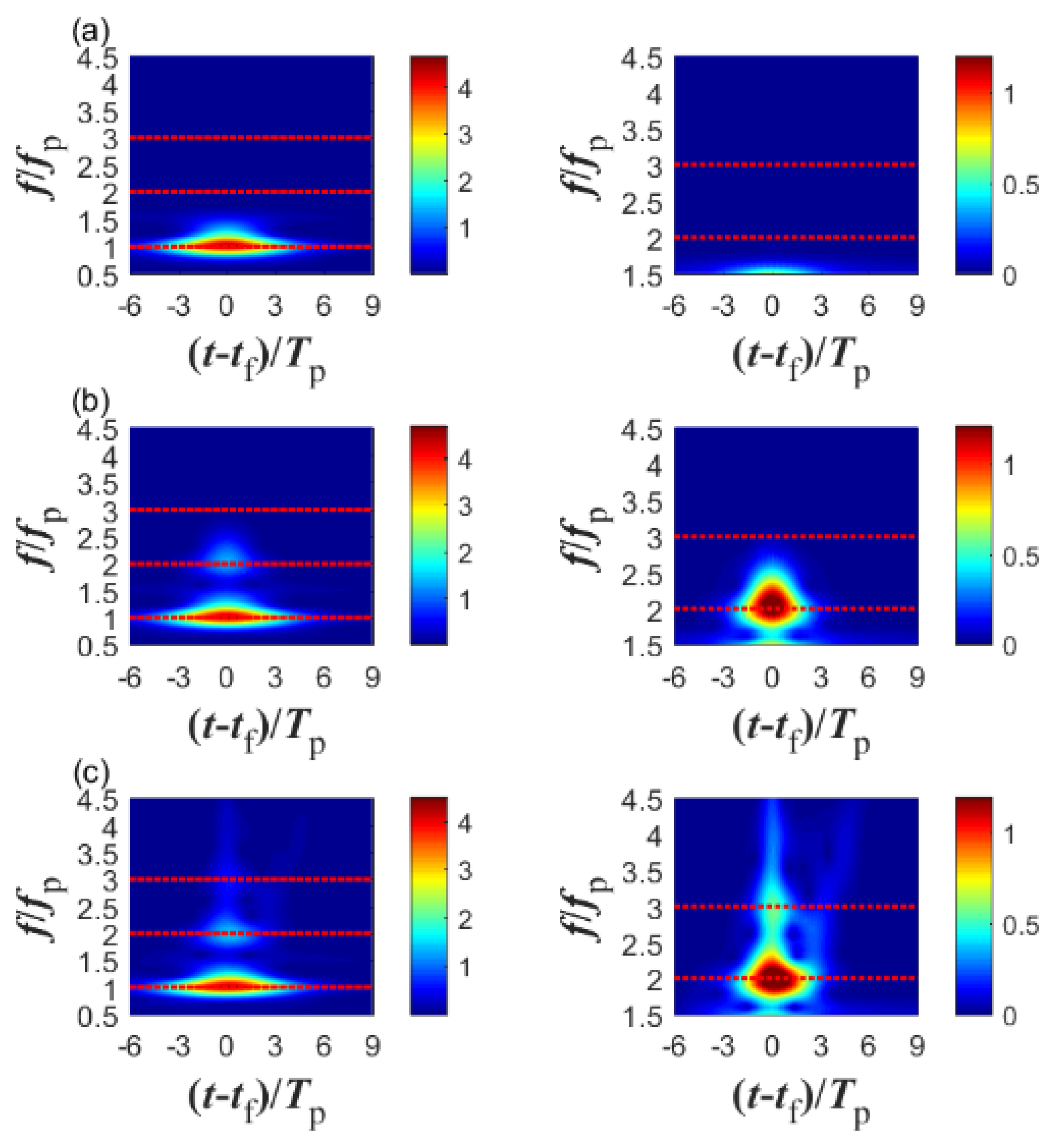
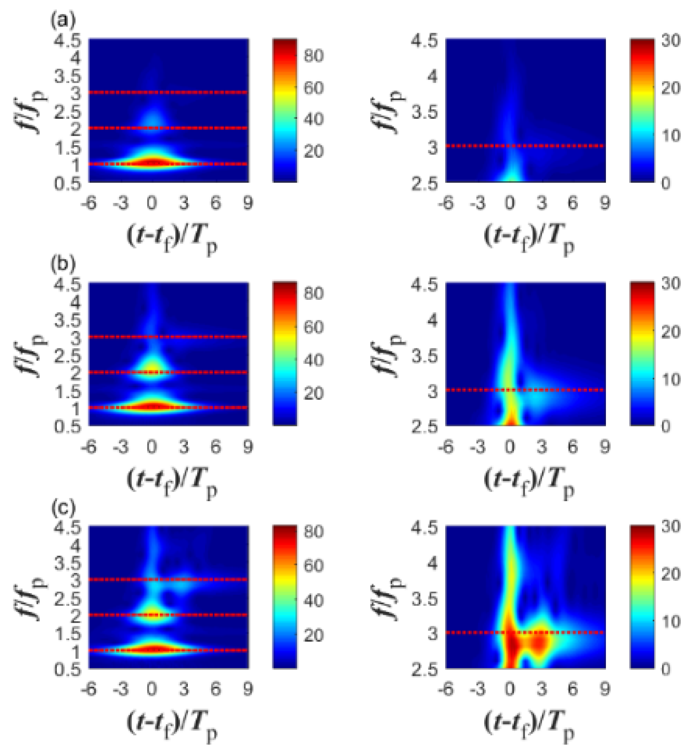
2.3. Wavelet Transform-Based Analyses

The wave loads and the related ringing response are transient phenomena rather than stationary processes. To investigate their local characteristics, the wavelet transform, which can generate localized time–frequency information from time series, is adopted. The continuous wavelet transform is defined by the inner product of a time function χ(t) and a family of continuously translated and dilated wavelets ψ_a,τ(t):

$$WT(a,\tau )={\displaystyle {\int }_{-\infty }^{\infty }\chi }(t){\psi }_{\mathrm{a},\mathsf{\tau }}^{*}(t)\mathrm{d}t,$$

(43)

where the asterisk * denotes the complex conjugate. A family of functions ψ_a,τ(t), called “wavelets”, can be constructed by translating in time τ and dilation with scale a of a specified mother wavelet ψ(t). The scale a is interpreted as the reciprocal of frequency, f ≈ 1/a. The ψ_a,τ(t) expression is defined as:

$${\psi }_{\mathrm{a},\mathsf{\tau }}(t)=\frac{1}{\sqrt{a}}\psi \left(\frac{t-\tau }{a}\right).$$

(44)

One of the most extensively used mother wavelets in continuous wavelet analysis is the Morlet wavelet [27]. The complex Morlet wavelet is a plane wave modulated by a Gaussian envelope:

$$\psi (t)={\pi }^{-1/4}\exp \left(-\frac{t^2}{2}\right)\exp \left(i{\omega }_{0}t\right),$$

(45)

where ω₀ is the center frequency of the wavelet, usually chosen to be 6.0, to meet the allowable conditions [28].

3. Comparisons and Verifications

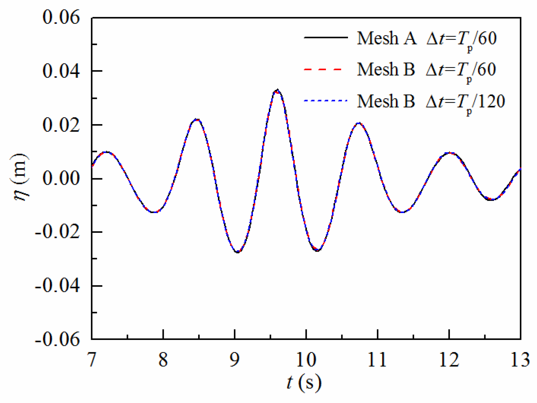
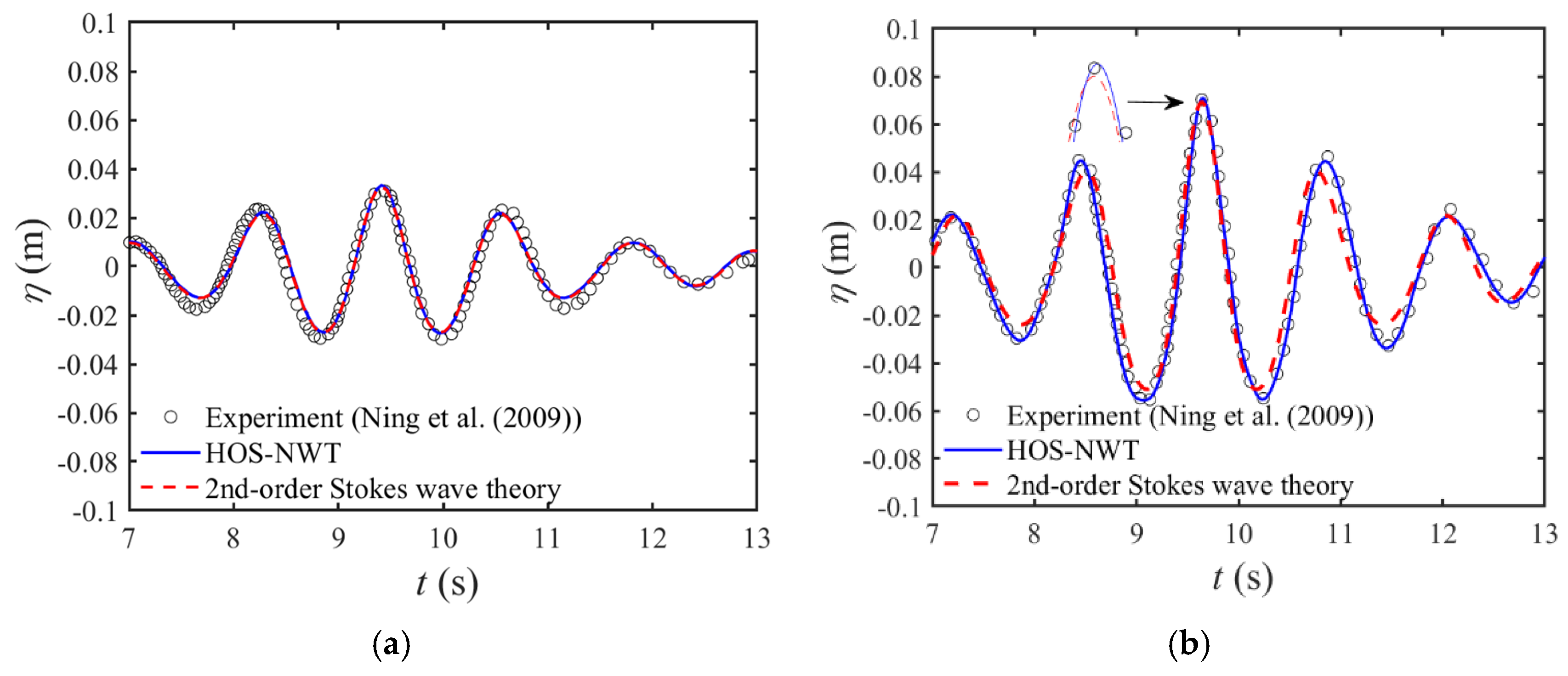
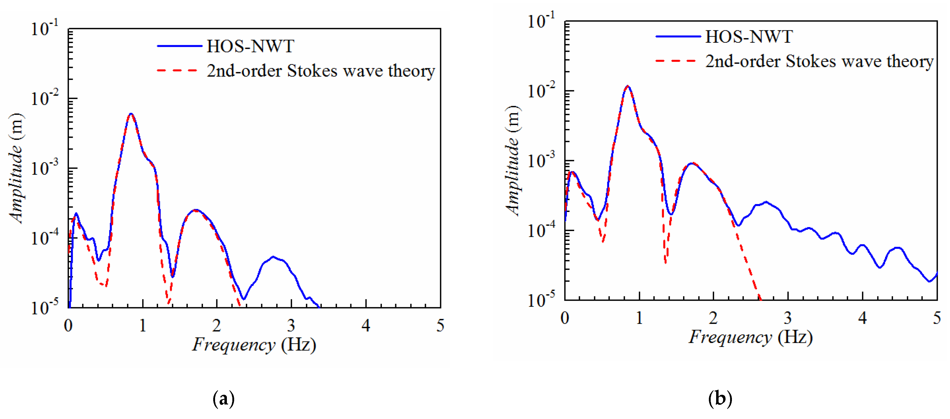
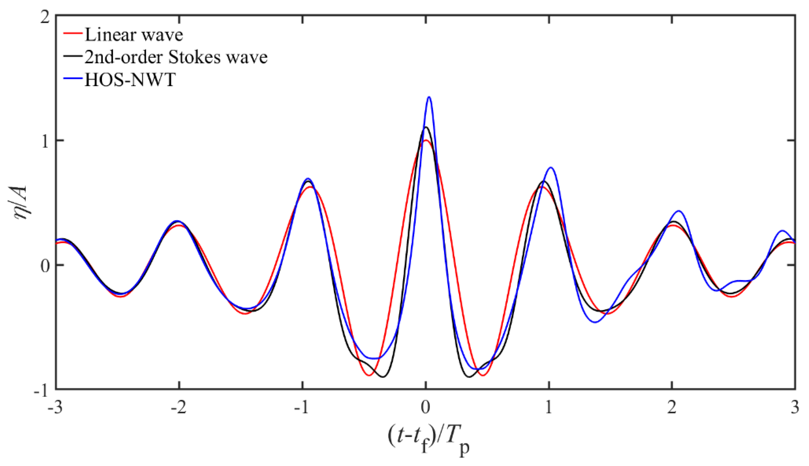
3.1. Validation Tests of Focused Wave Groups

The capability of the proposed formulation for focused wave group generation is verified here and compared with the experimental results from Ning et al. [16]. In the physical experiment, the wave flume is 69 m long and 3 m wide, and the maximum working depth is 1.5 m. The present study only focused on Cases 1 and 2 from the work by Ning et al. The water depth used in the experiments was d = 0.5 m. The details of the chosen focused wave groups are given in

Table 1. Parameters of the focused wave groups.

Case (Ning et al. [16])	Frequency Band f (Hz)	Peak Frequency fp (Hz)	Input Amplitude AI (m)
1	0.60 ≤ f ≤ 1.20	0.83	0.0313
2	0.60 ≤ f ≤ 1.30	0.83	0.0632

. The peak frequency f_p = 0.83 Hz (corresponding to wavelength L_p = 2.0 m and wavenumber k_p = 3.14 m⁻¹). The dimensionless wave steepness is defined as ε = k_pA_I = 0.10 for Case 1 and ε = k_pA_I = 0.20 for Case 2.

In the numerical simulation, the length of the tank is selected as 10 times the characteristic wavelength (10L_p), of which 4L_p is used as a damping layer at the downstream end of the tank to dissipate the outgoing waves, and the depth is 0.5 m. Each focused wave group consisted of 25 wave components, and the focus position and focus time are defined as x_f = 1.5L_p and t_f = 8T_p, respectively. At the start of the computation, a ramp function is applied over a time 2T_p to prevent any impulse-like behavior at the flux input boundary and to reduce the corresponding unnecessary transient waves. First, for the convergence analysis, Figure 5 shows the time series of free-surface elevations of Case 1 from the work by Ning et al. [16], calculated using two different mesh sizes and two different time steps. For Mesh A, results are performed with N_x = 512 (i.e., ≃52 modes per wavelength), and N_z = 128 vertical modes on the wavemaker. The number of modes of Mesh B (N_x = 1024, and N_z = 256 vertical modes on the wavemaker) is twice that of Mesh A. The time steps were selected as Δt = T_p/60 and Δt = T_p/120. Figure 5 shows that the results are almost identical, indicating that the numerical result is convergent using Mesh A, with Δt = T_p/60. The same grid and time step were adopted in the following simulation for Case 2.

The simulation results were compared with Cases 1 and 2 laboratory data from Ning et al. [16] and the input theoretical calculations in Figure 6. The present numerical results of Case 1 agree well with the second-order analytical solutions and the experimental measurements. Because the amplitude of the individual wave components was small, the effects of nonlinear wave–wave interactions were also very small. For Case 2, the wave crest at the focal point was larger and narrower, and the wave trough became wider and flatter, i.e., stronger nonlinearity. The present results agree quite well with the experimental measurements in terms of the wave crest, trough, and phase. The second-order analytical solution, whose shape is always perfectly symmetric, underestimates the main wave crest and troughs. In addition, there is a small phase difference when using it. Thus, the results of HOS-NWT are superior to the theoretical second-order Stokes wave, which is convincing evidence of the generation of focused wave groups in the HOS-NWT.

Different types of wave nonlinearity can be easily discerned in corresponding amplitude spectra in Figure 7a,b. Starting from low frequency, the main components of the focused wave groups contain a second-order difference term, a linear term, and a second-order sum term, where the present numerical results are consistent with the input second-order analytical solution. The smaller third-order sum terms and even the fourth-order terms can also be discerned with a larger wave steepness.

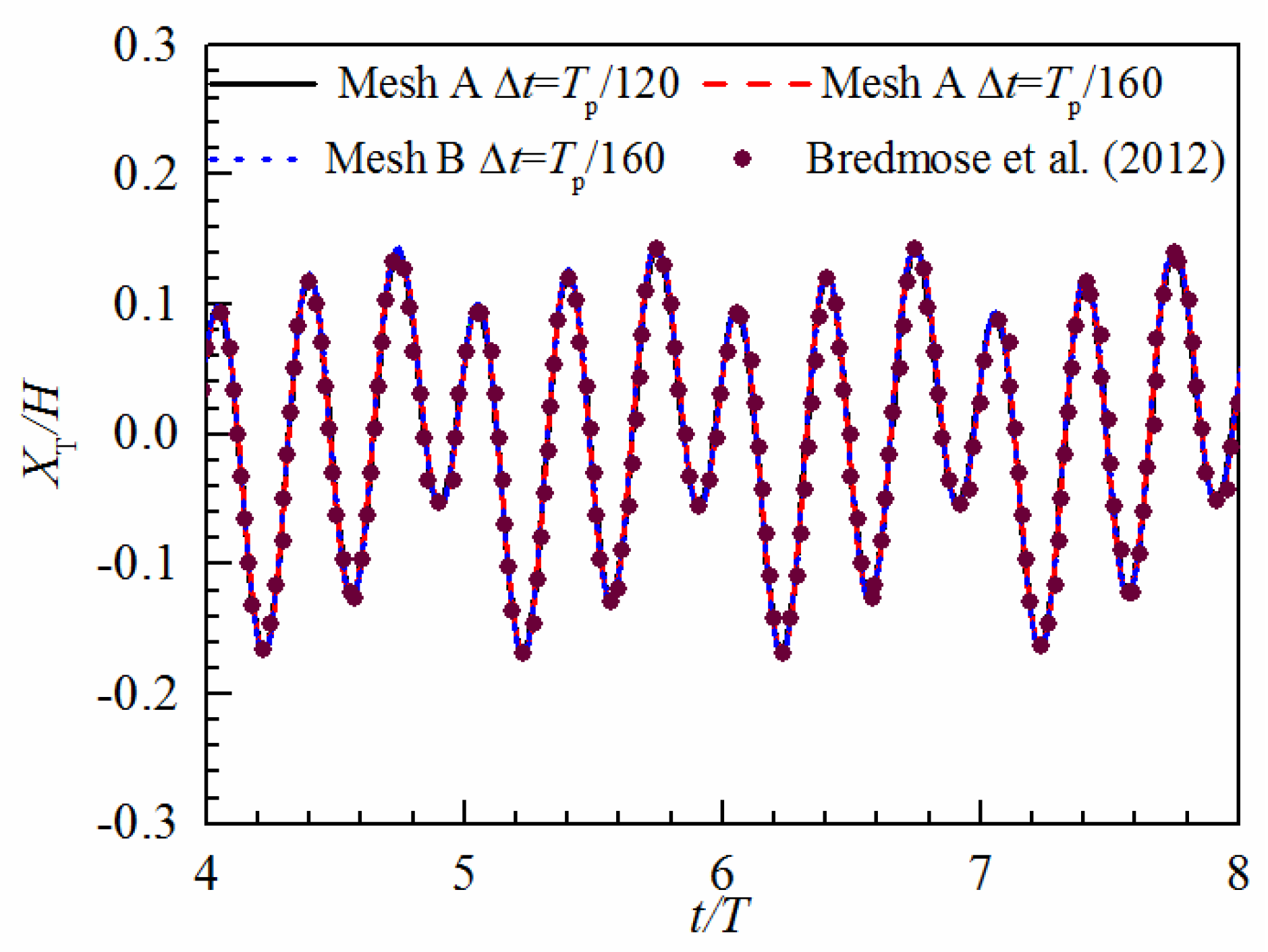
3.2. Validation Tests of Hydro-Elastic Model

The ability of the hydro-elastic model to predict the monopile response to nonlinear wave forcing can be validated by comparing the results with those of Bredmose et al. [3]. The main simulation parameters were chosen based on a typical offshore wind turbine foundation: a depth of d = 20 m, a diameter of D = 5 m, a length of l = 40.0 m, g = 9.81 m/s², density of water ρ = 1025 kg/m³, structural mass per unit length $\overline{m}$ = 20,000.0 kg/m³, and the flexural rigidity of section EI = 10219084252.53 N/m². As a result, the natural frequency of the monopile was set as f₁ = 0.25 Hz. The above parameters were used for all the following simulations. The regular wave parameters were set as wave height H = 5.00 m, wave length L = 155.91 m, wave period T = 12 s, and wave frequency f = 1/12 Hz, along with f₁/f = 3.0. The dependence of the results on the mesh size and time step was carefully checked by performing a convergence study. Equation (40) was discretized spatially using the finite-element method, with 200 Euler beam elements for Mesh A and 300 Euler beam elements for Mesh B. The time step interval was set as Δt = T/120 and Δt = T/160. The time series of the top-point motion X_T, normalized with wave height, are presented in Figure 8. One can see that the numerical result is convergent using Mesh A, with Δt = T/120, which is adopted in the work discussed in Section 4. Overall, a satisfactory agreement with Bredmose et al. was reached, demonstrating the feasibility of the present hydro-elastic model for the monopile.

4. Numerical Results and Discussion

The ringing response induced by the third-order harmonic wave loads of focused wave groups generated in the HOS-NWT was investigated, and the results are discussed in this section. The simulation parameters of the monopile are the same as those in Section 3.2. The peak spectral frequency of the incident focused wave group was set to one-third of the natural frequency of the monopile, i.e., f_p = f₁/3 = 1/12 Hz. The focused wave group consisted of 25 continuous sinusoidal components whose frequencies were equally spaced within the range 0.5f_p < f < 1.5f_p. The wave number k_p = 0.0412 m⁻¹ is the linear dispersion wave number corresponding to f_p, along with the wavelength L_p = 152.33 m. Following Ning et al. [16], the focus position, where the monopile is placed, and focus time are defined as x_f = 1.50L_p and t_f = 8T_p, respectively. The length of the wave tank was L = 10L_p = 1523.30 m. The length of the damping zones at the end of the computation domain was 4L_p. The simulations covered seven different input amplitudes A. Detailed information is listed in

Table 2. Parameters of the generated waves.

Case	1	2	3	4	5	6	7
A (m)	0.5	1.5	2.5	3.1	3.5	4	4.4
kpA	0.02062	0.06186	0.10310	0.12743	0.14393	0.16496	0.18145

.

The time sequence of the surface elevation at the focus position, with the highest input amplitude (i.e., Case 7), and the corresponding wavelet spectrum are shown in Figure 9 and Figure 10. In Figure 9, the results are compared with the linear, second-order solutions. The numerically calculated crest of focused wave groups is higher and narrower, while troughs become wider and shallower than those of theoretical solutions, which is attributed to the nonlinear interaction between wave components. In Figure 10, the color bar indicates the modulus of the wavelet coefficients, and the image on the right is a partial enlarged view of the left image for higher-order components in the normalized frequency range of 1.5~4.5. The wavelet analysis results show that only the first and second-harmonic components of focused wave groups are evident for theoretical solutions. However, the third and fourth harmonics appear using the focused wave generated in the HOS-NWT.

The dimensionless maximum crest elevations versus the wave steepness k_pA are shown in Figure 11. The dimensionless maximum crest elevations are further enhanced by increasing the input amplitude, indicating that the nonlinearity of the freak wave increases with the wave steepness.

4.1. Damping Ratio Study

Although the damping of the monopile is typically low [29], it has a significant effect on the resonant response. Different damping ratios ξ = 0.00, 0.01, 0.02, and 0.05 for Case 7 were investigated. The time histories of the sectional moment at the base, calculated using Rainey’s model with focused wave groups generated in the HOS-NWT, and the corresponding wavelet spectrum are shown in Figure 12 and Figure 13. In Figure 13, the image on the right is a partial enlarged view of the left image for higher-order components in the normalized frequency range of 2.5~4.5. Figure 12 shows that the magnitude of the damping ratio has a slight influence on the peak of the wave loads. From the wavelet spectrum in Figure 13, one can see that the wave load is dominated by the first-order component, and the higher-order components of wave loads are much smaller, as expected. Their wavelet amplitudes in the freak wave region are more concentrated, larger in amplitude, and wider in frequency band, which indicates that considerable high-order harmonic overturning moments tend to appear in waves with transient characteristics. In Figure 13, another larger peak of the third-order moment after the first peak can be found with ξ = 0.00.

The top-point motion and corresponding wavelet spectrum are shown in Figure 14 and Figure 15. Figure 14 shows that the ringing phenomenon is obvious. The oscillation of the beam bursts a little after the focus time and lasts for several peak wave periods, which indicates that the ringing response occurs immediately after the incident wave crest passes the location of the monopile. As the damping ratio increases, the burst motions of the monopile are almost constant; however, the duration of the subsequent resonant response is much shorter compared with that of the pattern obtained without considering the damping. Figure 15 shows that, although the first- and second-harmonic components of wave loads are predominant, the response induced by them is almost negligible, while the third one dominates the resonant response because of the dynamic amplification. After the focus time, the third-harmonic components appear to be quite significant and last for several peak periods. When a larger damping ratio is considered, the amplitudes of the third-order response are significantly reduced.

In addition, Figure 16 shows the top-point horizontal acceleration, which is further amplified owing to the ω² effect. The maximum horizontal acceleration can reach 0.53 g with ξ = 0.00. Therefore, the ringing response induced by the high-order wave loads will be noticed in the design and operation of monopiles.

In summary, the wavelet transform method is promising for providing reliable and rich detailed information for the characteristics of the higher-harmonic wave loads and ringing response. In the present study, following Bredmose et al. [3], a smaller value of damping ratio ξ = 0.01 is used in the following simulations.

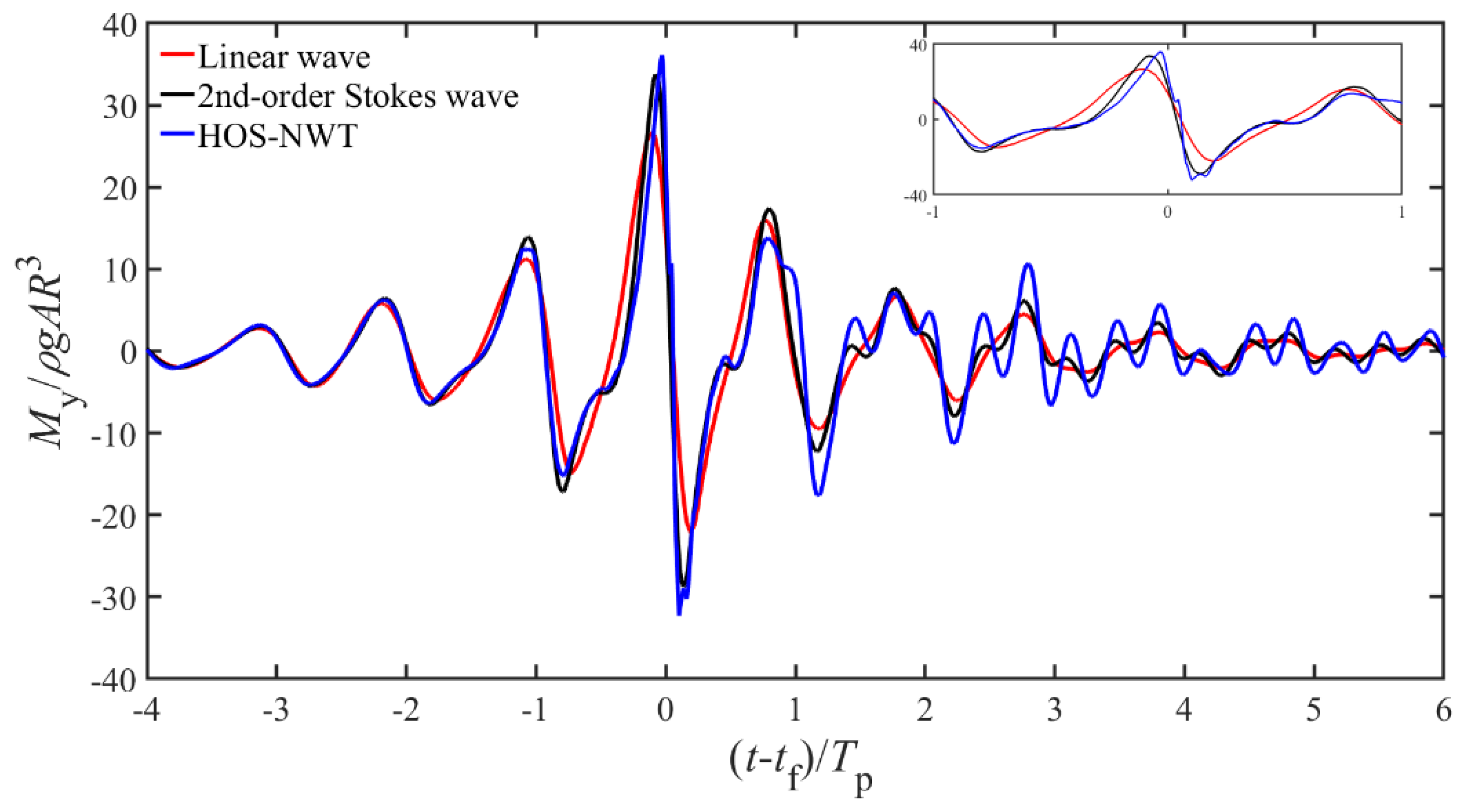
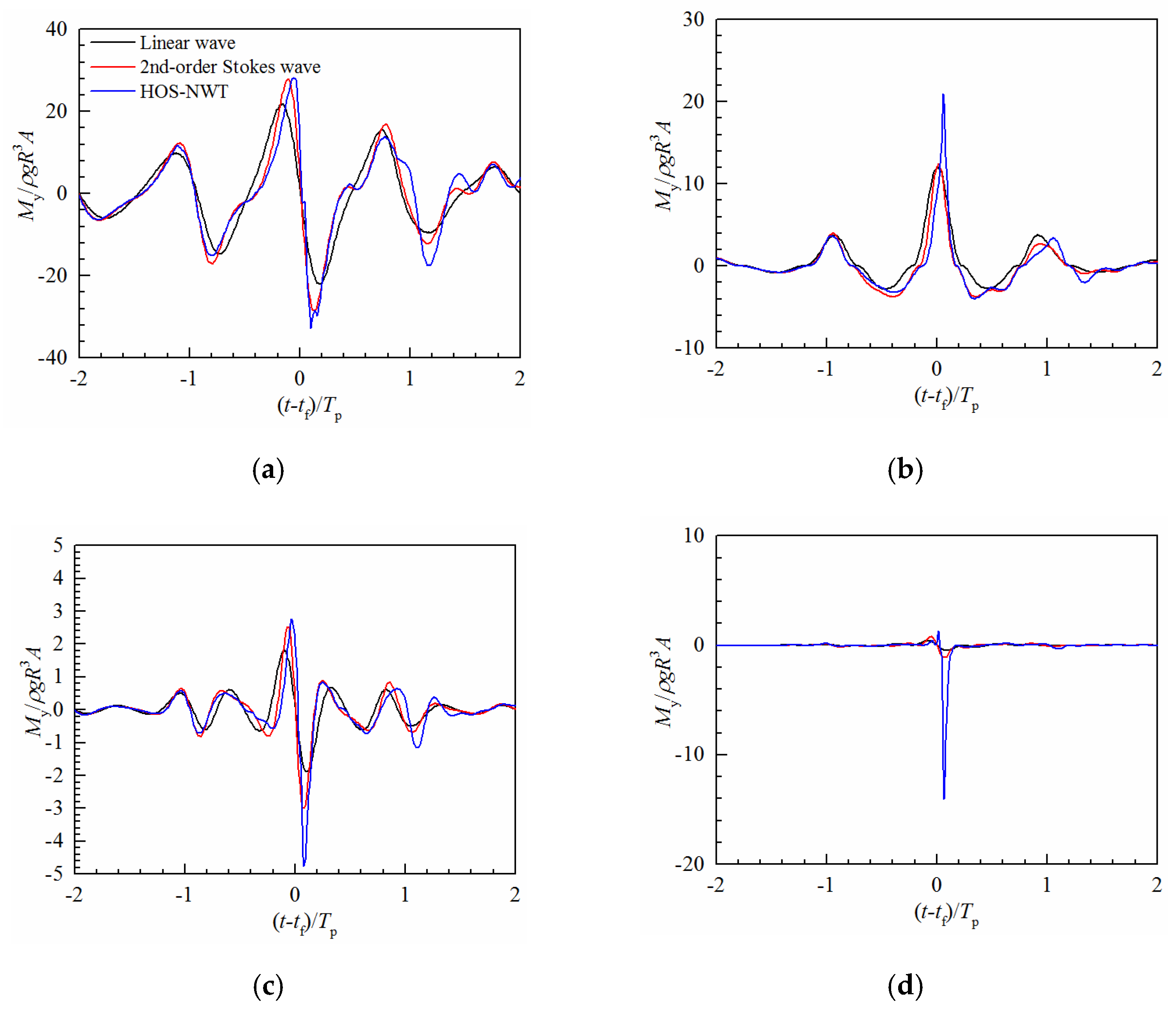
4.2. Different Wave Models for Wave Loads and Ringing Response

For the ultimate limit state, it is interesting to see how large the contribution from the nonlinearity of the incident wave for wave loads. The overturning moments for Case 7 are presented as an example, using Rainey’s model. In Figure 17, the differences between the different focused wave models are therefore easy to identify. There is an obvious secondary load cycle [30], which only occurs using focused waves generated in the HOS-NWT, suggesting the severest kinematics among the incident wave models and higher harmonics appearance. Its main peak moment is the largest among all three incident wave models. The wavelet spectra overturning moments were examined, as shown in Figure 18. The image on the right is a partial enlarged view of the left image for higher-order components in the normalized frequency range of 2.5~4.5. For the linear incident wave model, only the first-harmonic components are evident. For the second-order Stokes theory, except for the linear component, the second harmonic is also obvious. The third and fourth harmonics appear using the focused wave generated in the HOS-NWT.

Figure 19 presents the total moment and its components based on the focused wave groups generated in the HOS-NWT. It shows that the peak value of the total moment is dominated by the inertial part, and the peak of the inertial moment and the axial divergence moment appear in the rising phase of the focused wave groups, while the drag moment peak and the surface intersection moment trough are synchronized with the occurrence of the focused wave groups. Because of the reverse phase, although the peak value of the drag moment is considerable in this case, it contributes disproportionately to the peak of the total moment, which is still synchronized with the inertial part.

Comparisons of four components of the Rainey’s model using different incident wave models are shown in Figure 20a–d. For inertia-dominated structures, as here, the wave load depends more on the particle acceleration and, therefore, becomes larger the steeper the waves are. The inertial part is the cause of the secondary loading cycle. For the remaining three moments, the wave generated in the HOS-NWT gives the largest amplitude, owing to the severest kinematics, as explained above.

Figure 21 shows the time series of the overturning moment, using the focused wave groups generated in the HOS-NWT with different wave steepness. As the wave steepness increases, the peak moment (i.e., the maximum moment) tends to appear simultaneously with the occurrence of the focused wave groups, i.e., t = 8T_p. As the wave steepness decreases, the secondary loading cycle disappears. In Figure 22, the dimensionless peak moments are presented as a function of wave steepness. The dimensionless peak moment increases with an increase in the wave steepness. Based on the linear theory, the results should be independent of the wave steepness. Thus, the relationship between the peak nondimensional moment and wave steepness is strongly nonlinear rather than linear. In general, the ultimate loads calculated by the two different nonlinear wave theories agree with each other well. However, the discrepancies between the nonlinear and linear wave models increased monotonically with increasing wave steepness.

Figure 23 and Figure 24 show the time series of the dimensionless motion of the top-point and corresponding wavelet spectrum for Case 7. Figure 23 shows that the peak values of the dimensionless motion, using the focused wave groups generated in the HOS-NWT, are larger than those of the remaining two wave models. The linear wave model is in rather poor agreement with other nonlinear wave models. In Figure 24, the wavelet analysis shows that differences are obvious among different incident wave models. Second-order wave theory performs well for the prediction of peak wave loading, but it has poorer prediction of the ringing response because the higher harmonics of the moment are not captured, as shown in Figure 18. Therefore, the predictions of wave loads and induced responses are closely correlated with the incident wave model, and the fully nonlinear focused wave generated in the HOS-NWT are preferred as the incident focused wave model.

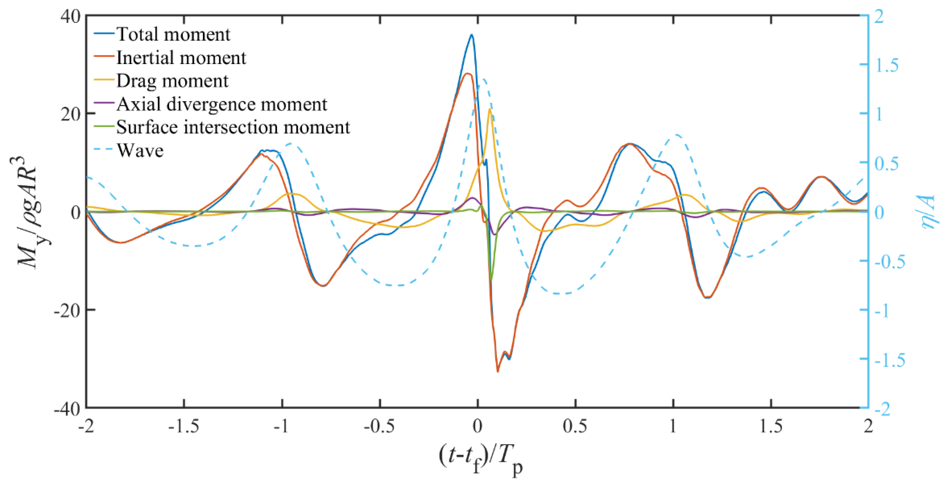
4.3. Different Hydrodynamic Models for Wave Loads and Ringing Response

The Morison equation and Rainey’s model, which contains two additional potential flow loads, i.e., the axial divergence part and surface intersection part, to improve accuracy, were applied in assessing the wave loads for comparison purposes. The nonlinear freak waves generated in the HOS-NWT were used as incident waves under Case 7 as an example. As shown in Figure 25, the results from the Morison equation and Rainey’s model agree well, except for the main peak and trough value. The Morison equation may underestimate the peak wave loads and trough wave loads. When the axial divergence part is considered, the peak overturning moment agrees better with Rainey’s model. In other words, the axial divergence part plays a more important role in prediction for peak wave loads, compared with the surface intersection part. Particular attention should be given to the secondary loading cycle, which appears even if only the Morison equation is considered. In Figure 26, the image on the right is a partial enlarged view of the left image for higher-order components in the normalized frequency range of 2.5~4.5. As shown in Figure 26, the first- and second-order components of the wavelet transform resulting from the Morison equation agree well with Rainey’s model, but the results around the higher frequency using Rainey’s model appear to be slightly larger because of the inclusion of slender-body terms.

Figure 27 shows the relationship between the peak nondimensional moment and the incident wave steepness using different hydrodynamic models. The predictions of Rainey’s model exceed those of the Morison equation by a margin that increases rapidly with wave steepness. The agreement is better when the axial divergence part is included, as explained above.

Figure 28 shows the time series of the dimensionless top-point motion. No matter which hydrodynamic model is used, the monopile is excited at its natural frequency, yielding a large ringing response. Similar to the wave loads in Figure 25, a higher peak is observed when using Rainey’s model compared with the Morison predictions after the focus time.

5. Conclusions

The ringing response of a monopile to higher-harmonic wave loads induced by fully nonlinear focused wave groups was investigated. This study reveals that for the steepest case, quantitatively, the largest absolute values of the normalized wave loads M_y (i.e., the main crest) using HOS-NWT are approximately 1.36 times that using the linear wave theory, and the largest absolute values of the normalized ringing response X_T (i.e., the main trough) using HOS-NWT are 2.68 times that using the linear wave theory. Wavelet-transform-based analyses were performed to investigate the local characteristics of the sectional moment at the base of a monopile and induced ringing response. The main conclusions drawn are as follows.

(1)

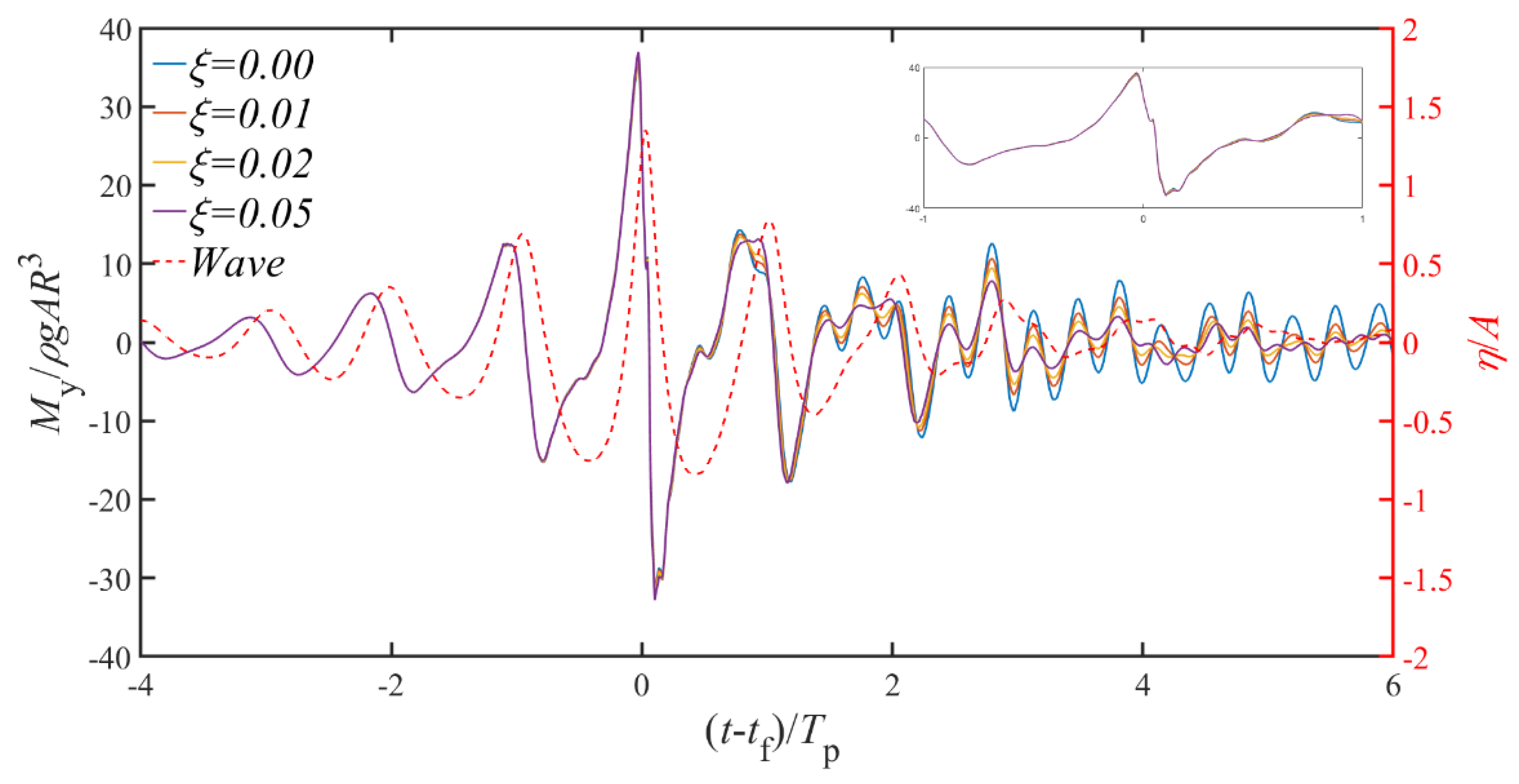
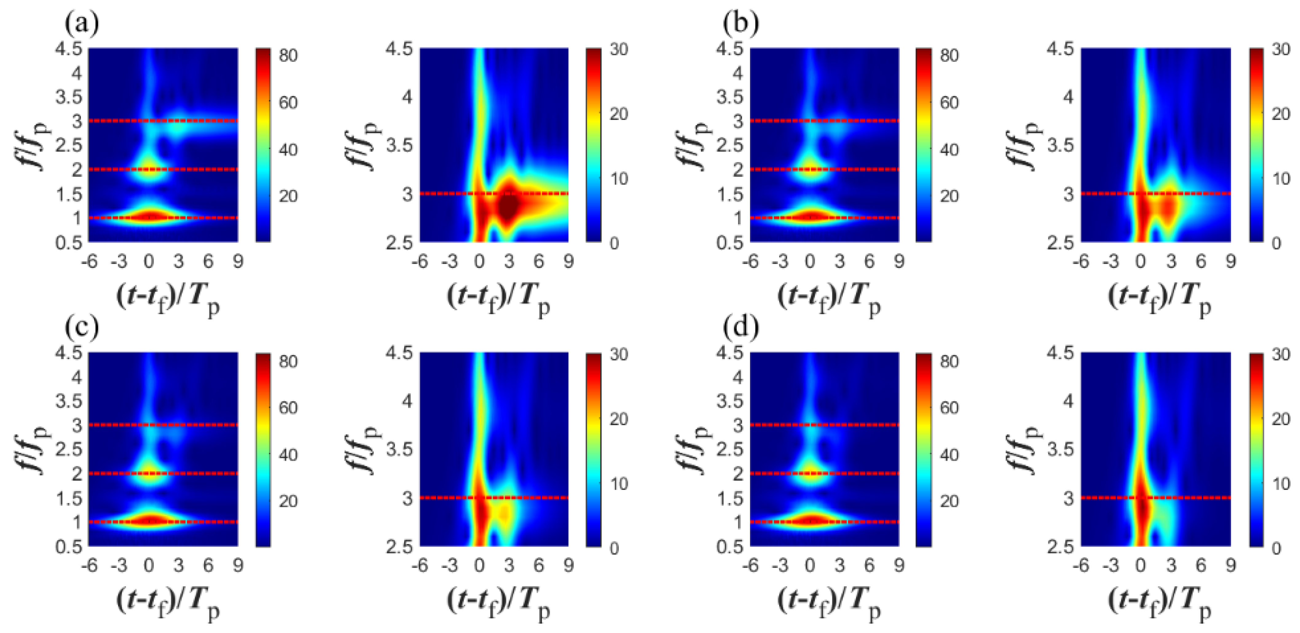
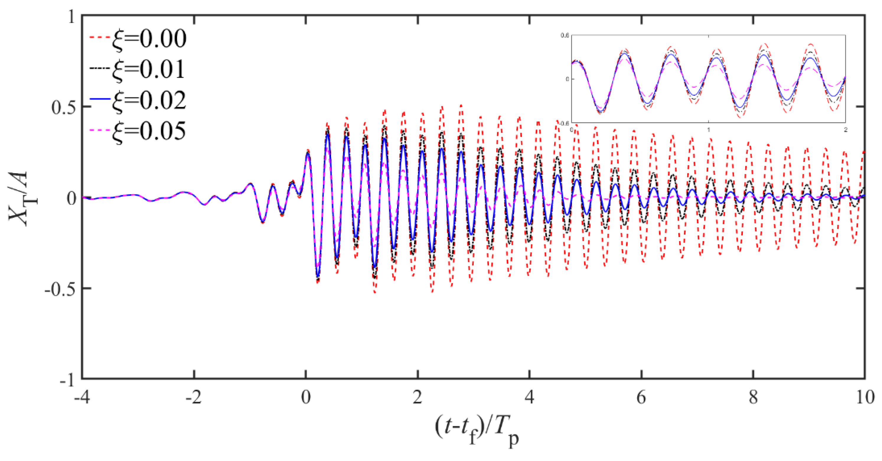
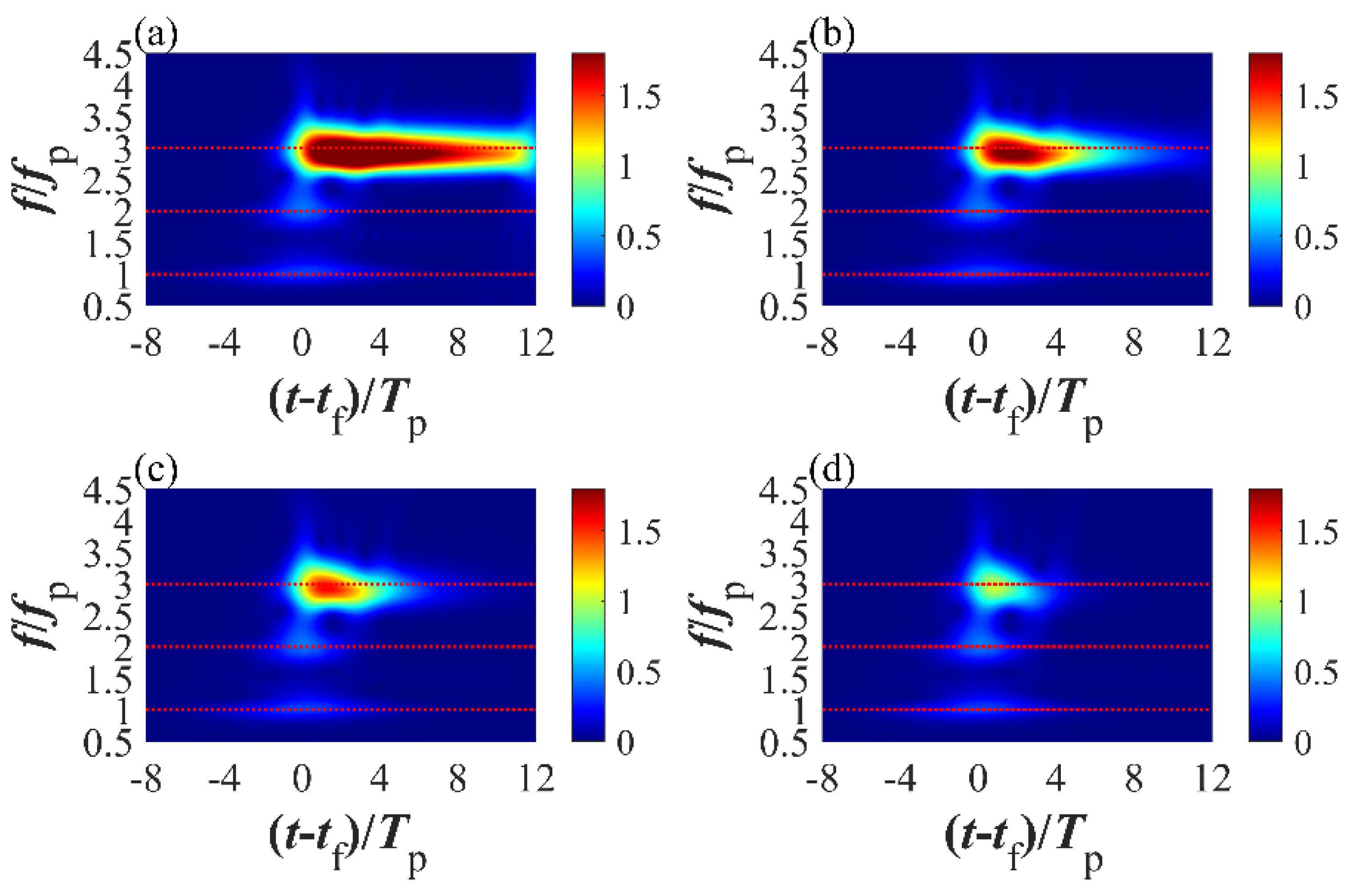
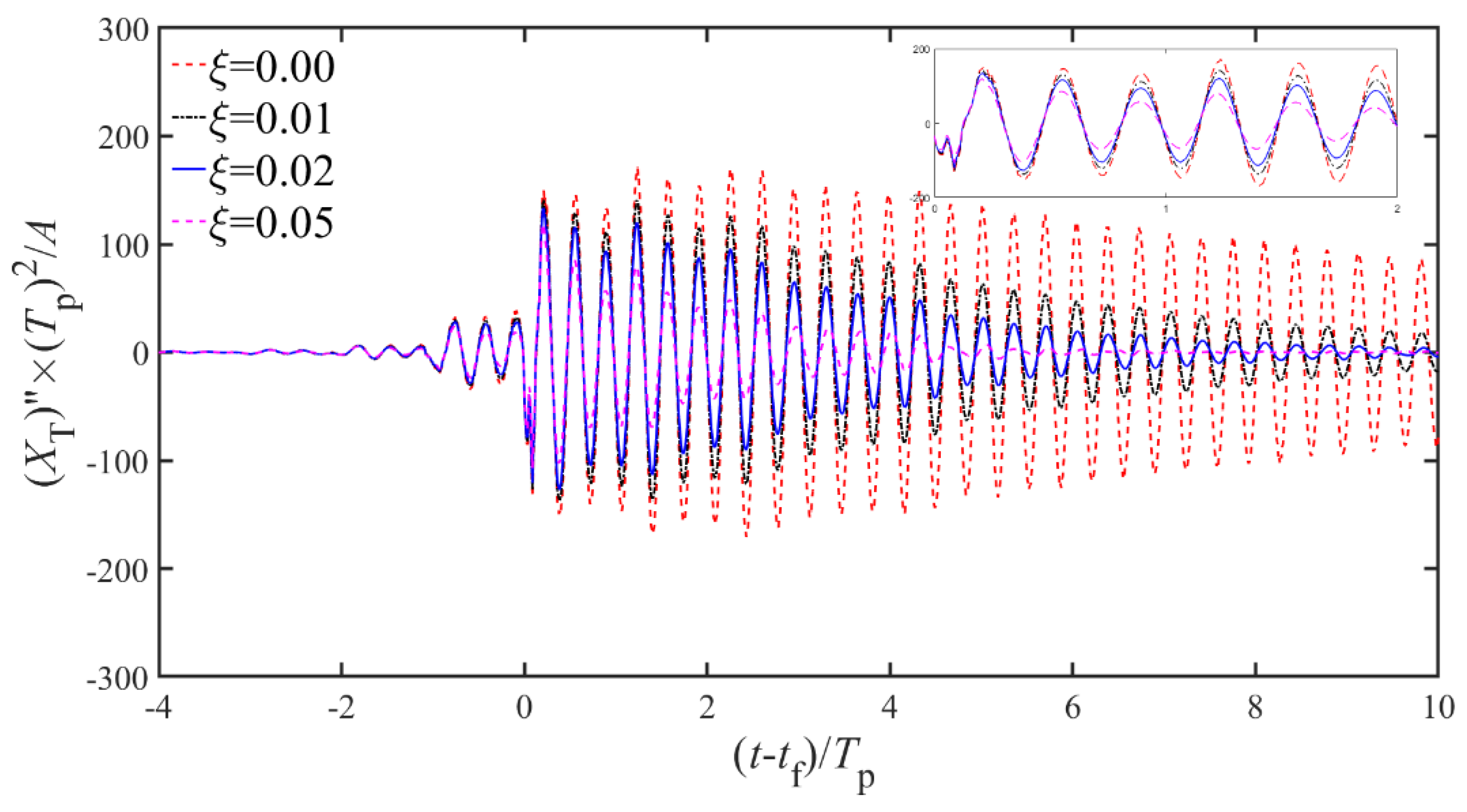
The magnitude of the damping ratio has a slight influence on the peak wave loads and induced response. However, a larger damping ratio leads to a faster decay of the subsequent resonance response.

(2)

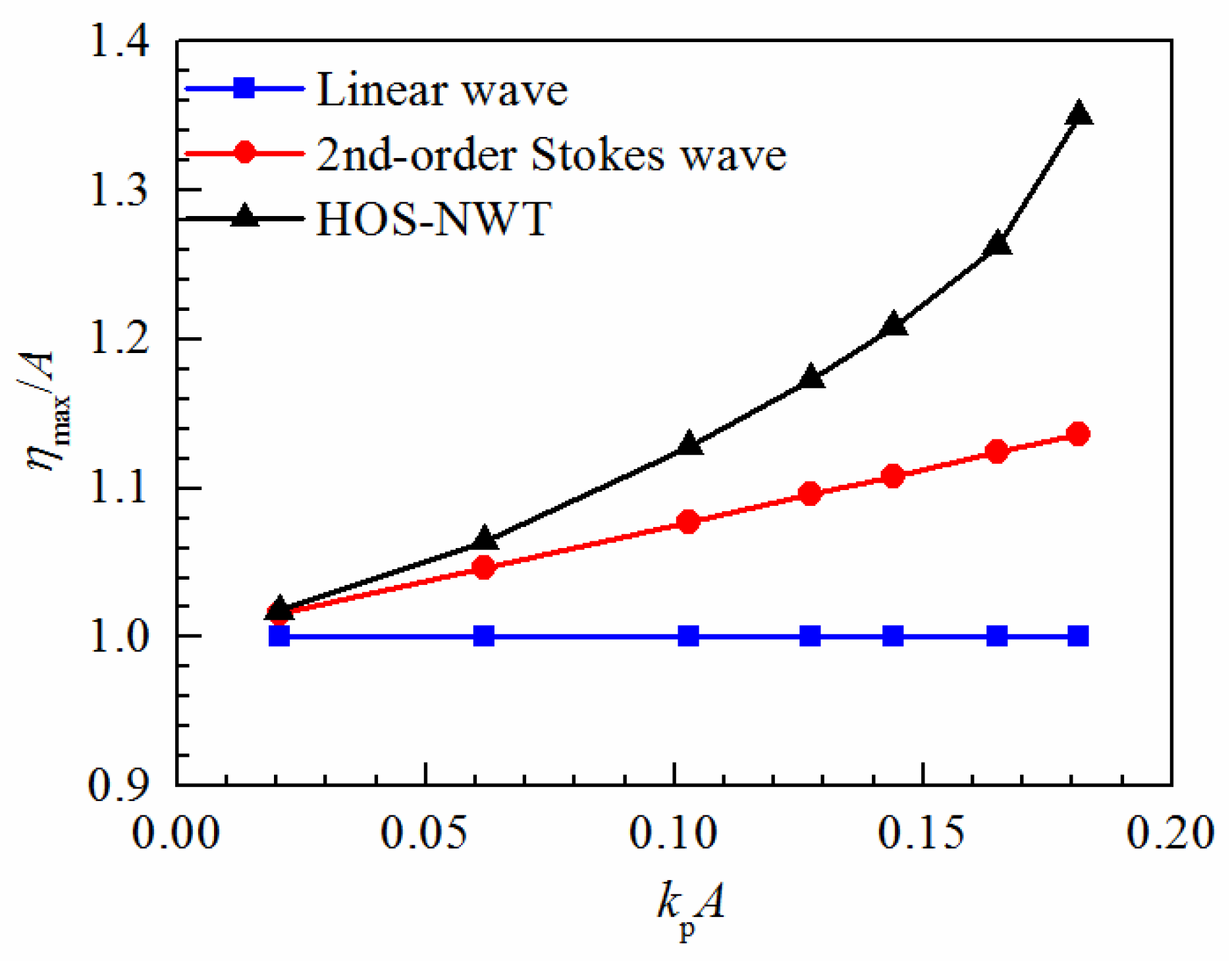
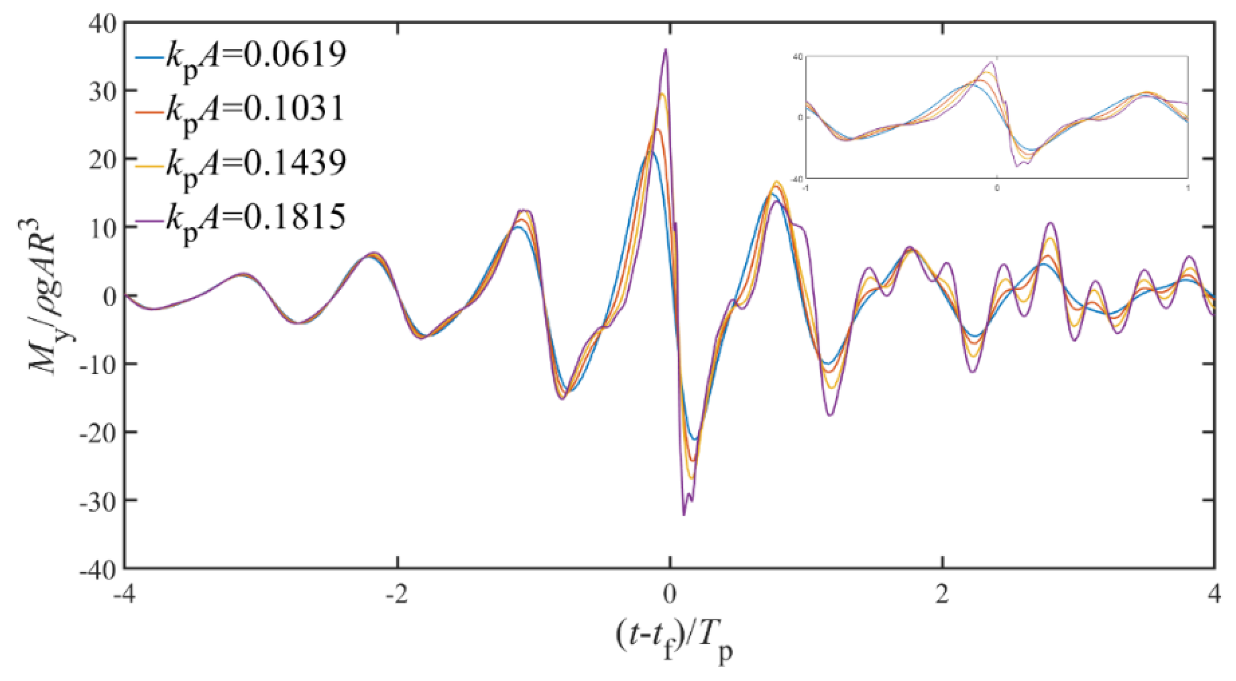
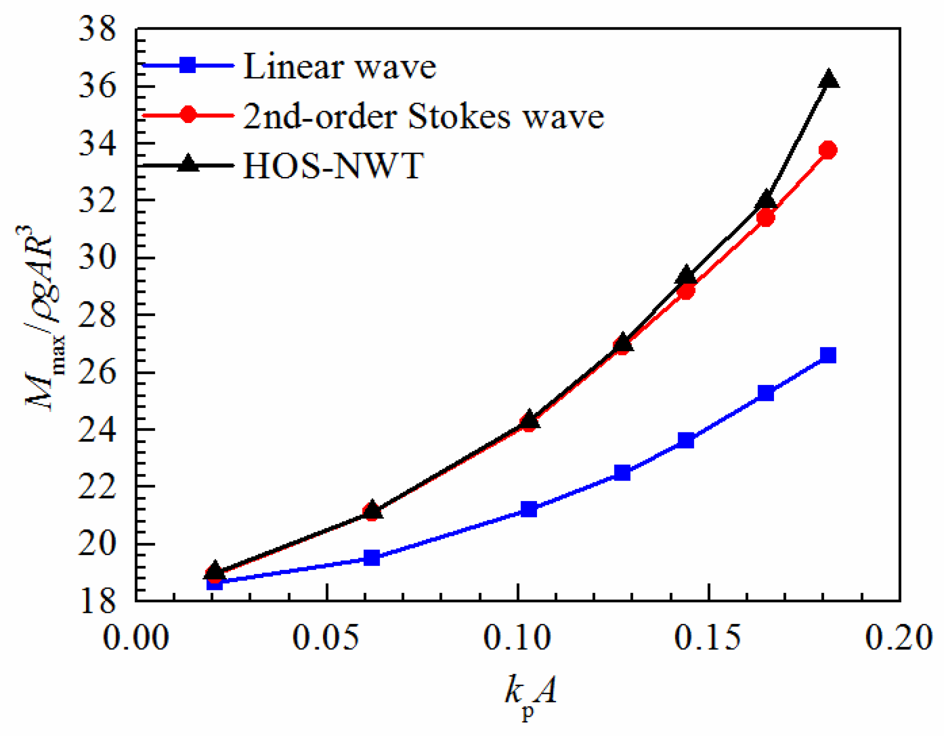
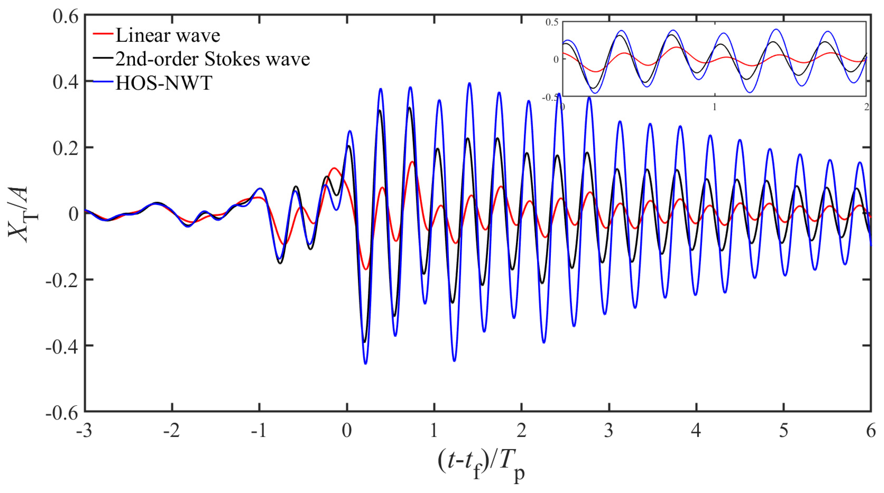
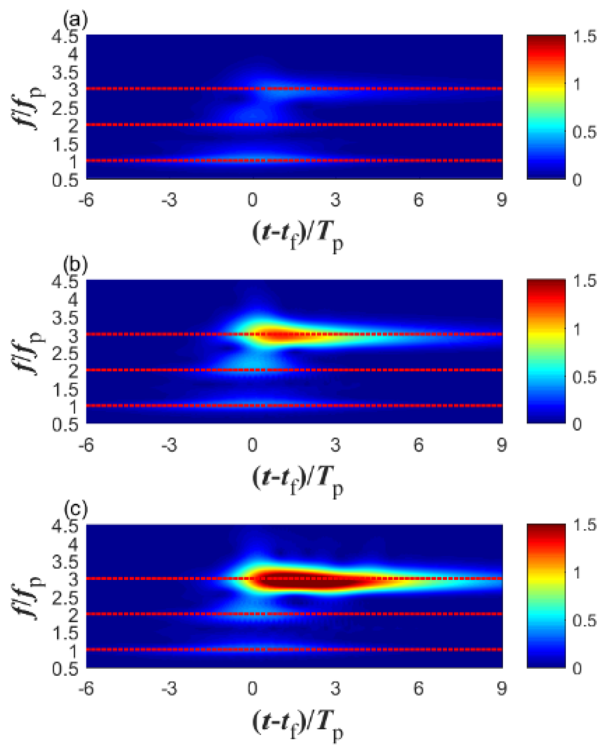
Nonlinear wave models are important for the prediction of ultimate wave loads and induced responses. The prediction of peak wave loads using nonlinear wave models exceeds that using a linear wave model by a margin that increases rapidly with wave steepness. Although second-order wave theory performs well for ultimate loads, it performs worse for the prediction of the ringing response because the higher harmonics of the moment cannot be captured.

(3)

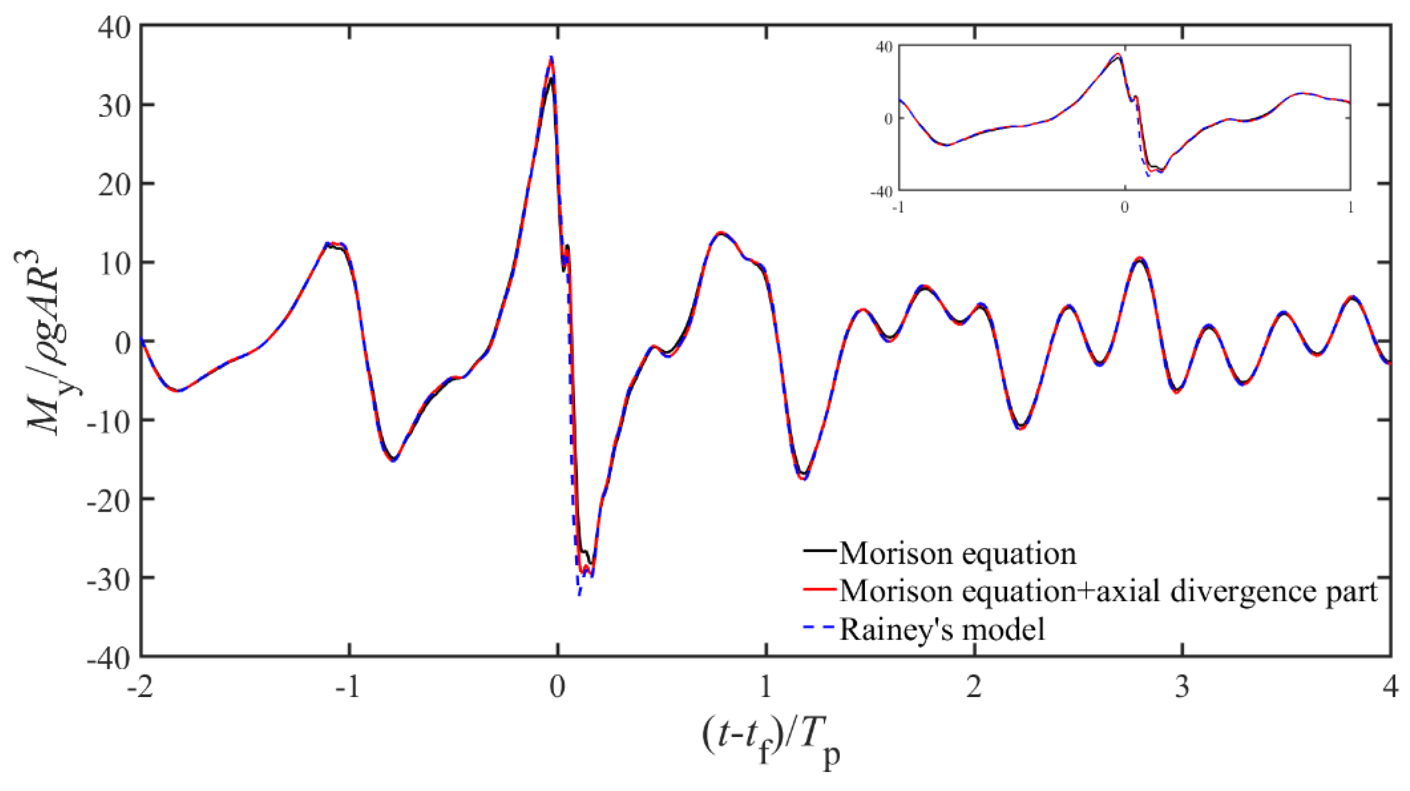
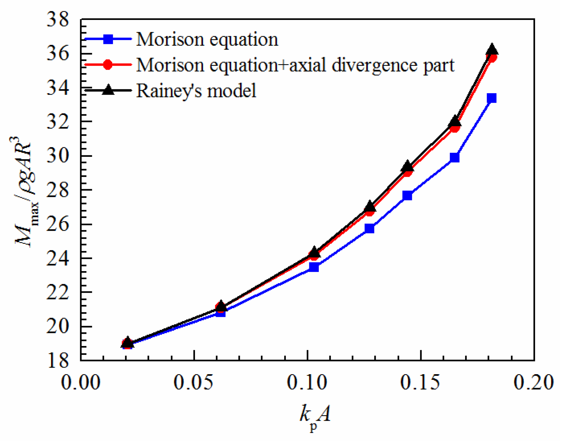
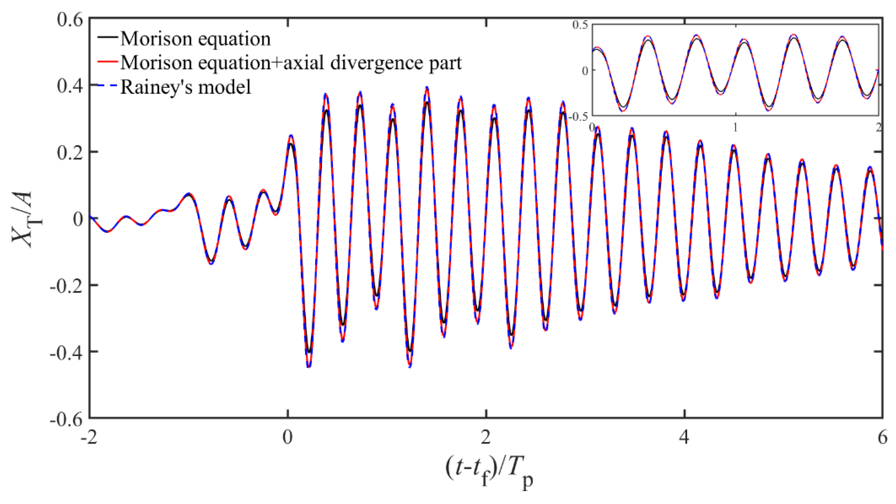
Rainey’s model gives a larger peak sectional moment than the Morison equation because of slender-body corrections, which are essential for accurate prediction of the wave loads. As a result, a higher peak of the dimensionless top-point motion was observed. The discrepancies in the dimensionless peak moments between the two hydrodynamic models tend to increase with wave steepness.

References

1. Ridder, E.J.D.; Aalberts, P.; Berg, J.V.D.; Buchner, B.; Peeringa, J. The dynamic response of an offshore wind turbine with realistic flexibility to breaking wave impact. In Proceedings of the ASME International Conference on Ocean, Offshore and Arctic Engineering, Rotterdam, The Netherlands, 19–24 June 2011. [Google Scholar]
2. Natvig, B.J.; Teigen, P. Review of hydrodynamic challenges in TLP design. Int. J. Offshore Polar Eng. 1993, 3, 294–302. [Google Scholar]
3. Bredmose, H.; Schløer, S.; Bo, T.P. Higher-harmonic response of a slender cantilever beam to fully nonlinear regular wave forcing. In Proceedings of the ASME International Conference on Ocean, Offshore and Arctic Engineering, Rio de Janeiro, Brazil, 1–6 July 2012. [Google Scholar]
4. Atkins, N.; Lyons, R.; Rainey, R. Summary of Findings of Wave Load Measurements on the Tern Platform; HSE Books: London, UK, 1997. [Google Scholar]
5. Rainey, R.C.T. A new equation for calculating wave loads on offshore structures. J. Fluid Mech. 1989, 204, 295–324. [Google Scholar] [CrossRef]
6. Rainey, R.C.T. Slender-body expressions for the wave load on offshore structures. Proc. R. Soc. A Math. Phys. Eng. Sci. 1995, 450, 391–416. [Google Scholar]
7. Manners, W.; Rainey, R.C.T. Hydrodynamic forces on fixed submerged cylinders. Proc. R. Soc. A Math. Phys. Eng. Sci. 1992, 436, 13–32. [Google Scholar]
8. Tromans, P.S.; Anaturk, A.R.; Hagemeijier, P. A new model for the kinematics of large ocean waves-application as a design wave. In Proceedings of the First International Offshore and Polar Engineering Conference, Edinburgh, UK, 11–16 August 1991. [Google Scholar]
9. Wang, W.; Kamath, A.; Pakozdi, C.; Bihs, H. Investigation of focusing wave properties in a numerical wave tank with a fully nonlinear potential flow model. J. Mar. Sci. Eng. 2019, 7, 375. [Google Scholar] [CrossRef] [Green Version]
10. Zijlema, M.; Stelling, G.S.; Smit, P.B. SWASH: An operational public domain code for simulating wave fields and rapidly varied flows in coastal waters. Coast. Eng. 2011, 58, 992–1012. [Google Scholar] [CrossRef]
11. Ducrozet, G.; Bonnefoy, F.; Touze, D.L.; Ferrant, P. A modified high-order spectral method for wavemaker modeling in a numerical wave tank. Eur. J. Mech. B Fluids 2012, 34, 19–34. [Google Scholar] [CrossRef]
12. Vyzikas, T.; Stagonas, D.; Buldakov, E.; Greaves, D. The evolution of free and bound waves during dispersive focusing in a numerical and physical flume. Coast. Eng. 2018, 132, 95–109. [Google Scholar] [CrossRef]
13. Vyzikas, T.; Stagonas, D.; Maisondieu, C.; Greaves, D. Intercomparison of three open-source numerical flumes for the surface dynamics of steep focused wave groups. Fluids 2021, 6, 9. [Google Scholar] [CrossRef]
14. Dommermuth, D.G.; Yue, D.K.P. A high-order spectral method for the study of nonlinear gravity waves. J. Fluid Mech. 1987, 184, 267–288. [Google Scholar] [CrossRef]
15. West, B.J.; Brueckner, K.A.; Janda, R.S.; Milder, D.M.; Milton, R.L. A new numerical method for surface hydrodynamics. J. Geophys. Res. 1987, 92, 11803–11824. [Google Scholar] [CrossRef]
16. Ning, D.Z.; Zang, J.; Liu, S.X.; Eatock Taylor, R.E.; Teng, B.; Taylor, P.H. Free-surface evolution and wave kinematics for nonlinear uni-directional focused wave groups. Ocean Eng. 2009, 36, 1226–1243. [Google Scholar] [CrossRef]
17. Dalzell, J.F. A note on finite depth second-order wave–wave interactions. Appl. Ocean Res. 1999, 21, 105–111. [Google Scholar] [CrossRef]
18. Rienecker, M.M.; Fenton, J.D. A fourier approximation method for steady water waves. J. Fluid Mech. 1981, 104, 119–137. [Google Scholar] [CrossRef]
19. Bonnefoy, F.; Touzé, D.L.; Ferrant, P. A fully-spectral 3d time-domain model for second-order simulation of wavetank experiments. Part a: Formulation, implementation and numerical properties. Appl. Ocean Res. 2006, 28, 33–43. [Google Scholar] [CrossRef]
20. Bonnefoy, F.; Touzé, D.L.; Ferrant, P. A fully-spectral 3d time-domain model for second-order simulation of wavetank experiments. Part b: Validation, calibration versus experiments and sample applications. Appl. Ocean Res. 2006, 28, 121–132. [Google Scholar] [CrossRef] [Green Version]
21. Goda, Y. A comparative review on the functional forms of directional wave spectrum. Coast. Eng. J. 1999, 41, 1–20. [Google Scholar] [CrossRef]
22. Agnon, Y.; Bingham, H.B. A non-periodic spectral method with application to nonlinear water waves. Eur. J. Mech. B Fluids 1999, 18, 527–534. [Google Scholar] [CrossRef]
23. Zakharov, V.E. Stability of periodic waves of finite amplitude on the surface of a deep fluid. J. Appl. Mech. Tech. Phys. 1968, 9, 190–194. [Google Scholar] [CrossRef]
24. Cash, J.R.; Karp, A.H. A variable order Runge–Kutta method for initial value problems with rapidly varying right-hand sides. ACM Trans. Math. Softw. 1990, 16, 201–222. [Google Scholar] [CrossRef]
25. Yamamoto, C.T.; Meneghini, J.R.; Saltara, F.; Fregonesi, R.A.; Ferrari, J.A. Numerical simulations of vortex-induced vibration on flexible cylinders. J. Fluids Struct. 2004, 19, 467–489. [Google Scholar] [CrossRef]
26. Newmark, N.M. A method of computation for structural dynamics. J. Eng. Mech. ASCE 1959, 85, 67–94. [Google Scholar]
27. Torrence, C.; Compo, G.P. A practical guide to wavelet analysis. Bull. Am. Meteorol. Soc. 1998, 79, 61–78. [Google Scholar] [CrossRef] [Green Version]
28. Farge, M. Wavelet transforms and their applications to turbulence. Annu. Rev. Fluid Mech. 1992, 24, 395–458. [Google Scholar] [CrossRef]
29. Kallehave, D.; Byrne, B.W.; LeBlanc Thilsted, C.; Mikkelsen, K.K. Optimization of monopiles for offshore wind turbines. Philos. Trans. R. Soc. Lond. A 2015, 373, 20140100. [Google Scholar] [CrossRef] [PubMed] [Green Version]
30. Grue, J.; Huseby, M. Higher-harmonic wave forces and ringing of vertical cylinders. Appl. Ocean Res. 2002, 24, 203–214. [Google Scholar] [CrossRef]
Figure 1. Definition sketch of coordinate system and computational domain.
Jmse 09 00286 g001
Figure 2. Wave tank scheme with its coordinate system.
Jmse 09 00286 g002
Figure 3. Extended domain Dadd for additional problem solution.
Jmse 09 00286 g003
Figure 4. Solution algorithm for the HOS-NWT approach.
Jmse 09 00286 g004
Figure 5. Convergence study of free-surface elevation for Case 1 from Ning et al. [16].
Jmse 09 00286 g005
Figure 6. Comparisons of time series of free-surface elevation: (a) Case 1 and (b) Case 2 from Ning et al. [16].
Jmse 09 00286 g006
Figure 7. Comparisons of corresponding amplitude spectrum. (a) Case 1; (b) Case 2 from Ning et al. [16].
Jmse 09 00286 g007
Figure 8. Time series of the top-point motion of the monopile XT.
Jmse 09 00286 g008
Figure 9. Comparisons of Case 7 with different focused wave models.
Jmse 09 00286 g009
Figure 10. Wavelet transform results of dimensionless free-surface elevation of the focused wave groups: (a) linear wave theory, (b) second-order Stokes wave theory, and (c) nonlinear wave generated in the HOS-NWT.
Jmse 09 00286 g010
Figure 11. Crest elevations with different focused wave models versus wave steepness kpA.
Jmse 09 00286 g011
Figure 12. Time series of the overturning moment My for Case 7.
Jmse 09 00286 g012
Figure 13. Wavelet transform results of the dimensionless overturning moment My: (a) ξ = 0.00, (b) ξ = 0.01, (c) ξ = 0.02, and (d) ξ = 0.05.
Jmse 09 00286 g013
Figure 14. Time series of the top-point motion of the monopile XT for Case 7.
Jmse 09 00286 g014
Figure 15. Wavelet transform results of the dimensionless top-point motion of the monopile: (a) ξ = 0.00, (b) ξ = 0.01, (c) ξ = 0.02, and (d) ξ = 0.05.
Jmse 09 00286 g015
Figure 16. Time series of the top-point acceleration of the monopile (XT)” for Case 7.
Jmse 09 00286 g016
Figure 17. Time series of the overturning moment My for different incident wave models.
Jmse 09 00286 g017
Figure 18. Wavelet transform results of the dimensionless overturning moment My: (a) linear wave theory, (b) second-order Stokes wave theory, and (c) nonlinear wave generated in the HOS-NWT.
Jmse 09 00286 g018
Figure 19. Time series of the overturning moment My and its components based on the focused wave groups generated in the HOS-NWT for Case 7.
Jmse 09 00286 g019
Figure 20. Comparisons of four components based on different focused wave models for Case 7: (a) inertial moment, (b) drag moment, (c) axial divergence moment, and (d) surface intersection moment.
Jmse 09 00286 g020
Figure 21. Time series of the overturning moment My based on the focused wave groups generated in the HOS-NWT with different wave steepness.
Jmse 09 00286 g021
Figure 22. Peak normalized moments versus wave steepness.
Jmse 09 00286 g022
Figure 23. Time series of the top-point motion of the monopile XT using different wave models for Case 7.
Jmse 09 00286 g023
Figure 24. Wavelet transform results of the dimensionless top-point motion of the monopile XT for Case 7: (a) linear wave theory, (b) second-order Stokes wave theory, and (c) nonlinear wave generated in the HOS-NWT.
Jmse 09 00286 g024
Figure 25. Time series of the overturning moment My for Case 7 using different hydrodynamic models.
Jmse 09 00286 g025
Figure 26. Corresponding wavelet transform results of My for Case 7 using different hydrodynamic models: (a) Morison equation, (b) Morison equation plus axial divergence part, and (c) Rainey’s model.
Jmse 09 00286 g026
Figure 27. Peak normalized moments as a function of wave steepness, computed using different hydrodynamic models with focused wave groups generated in the HOS-NWT.
Jmse 09 00286 g027
Figure 28. Time series of the top-point motion of the monopile XT for different hydrodynamic models for Case 7.
Jmse 09 00286 g028