
Remote Sensing-Based Automatic Detection of Shoreline Position: A Case Study in Apulia Region

 , , ,
, , ,  and
and
Abstract
:1. Introduction
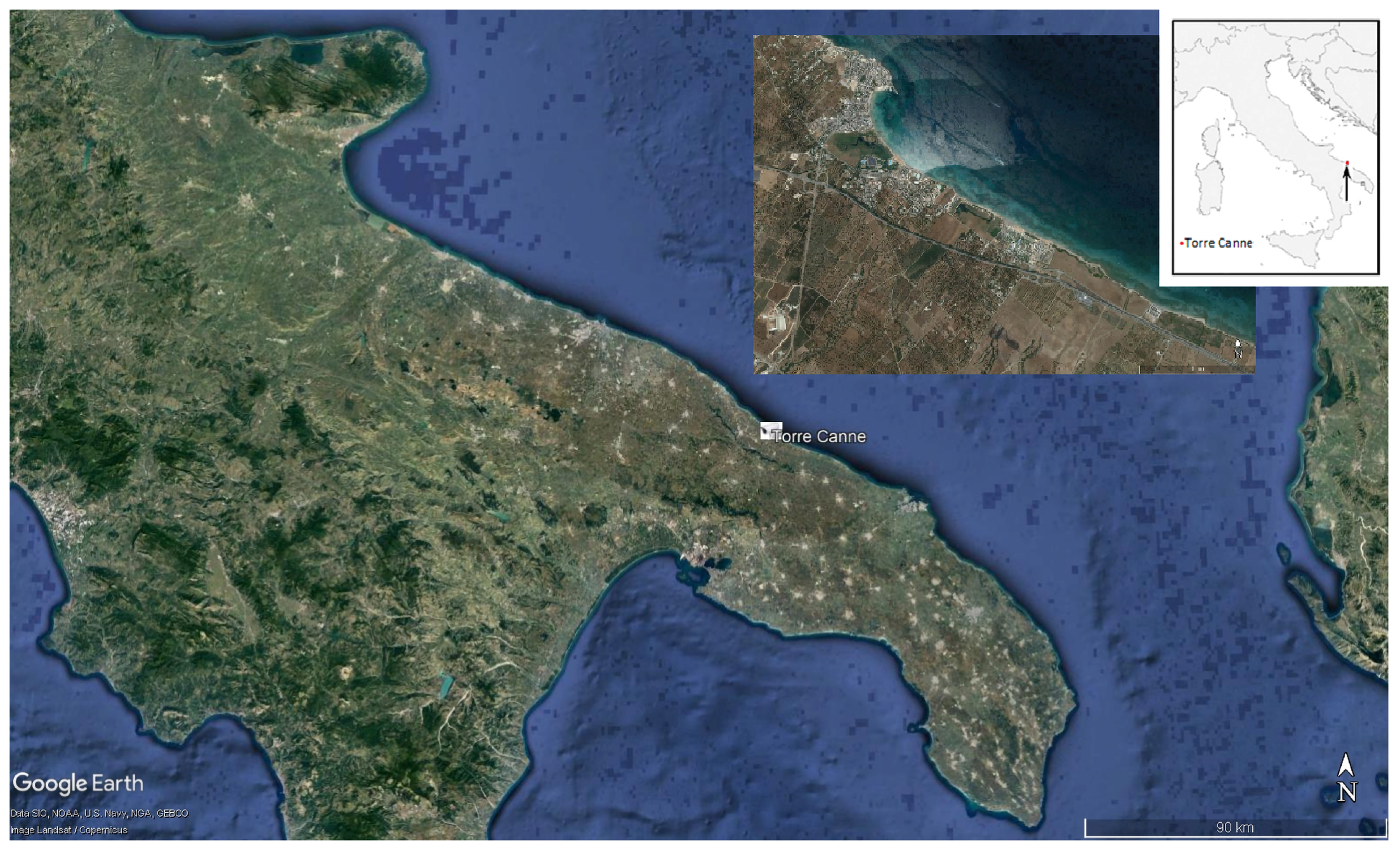
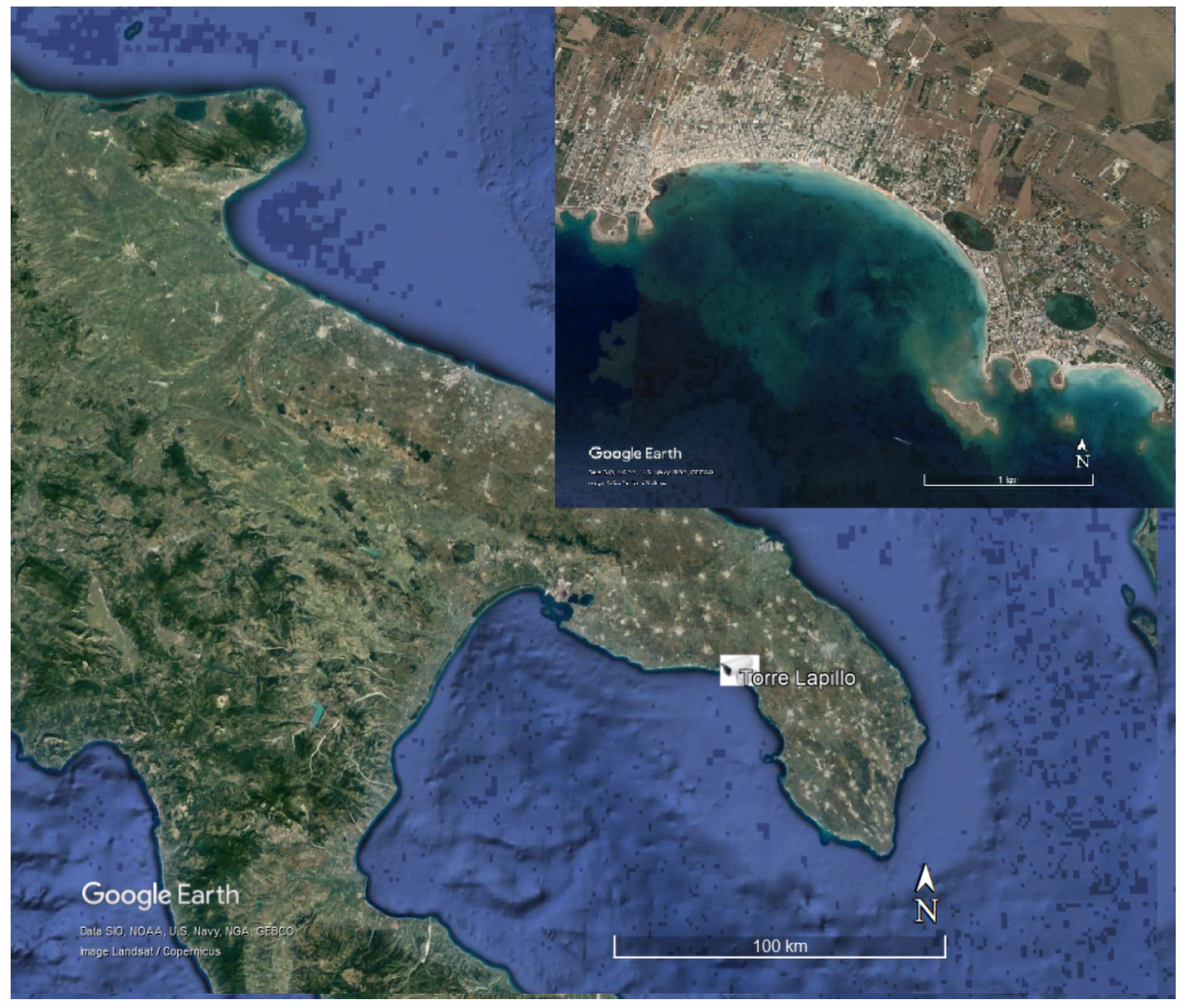
1.1. Study Area
2. Materials and Methods
2.1. Materials
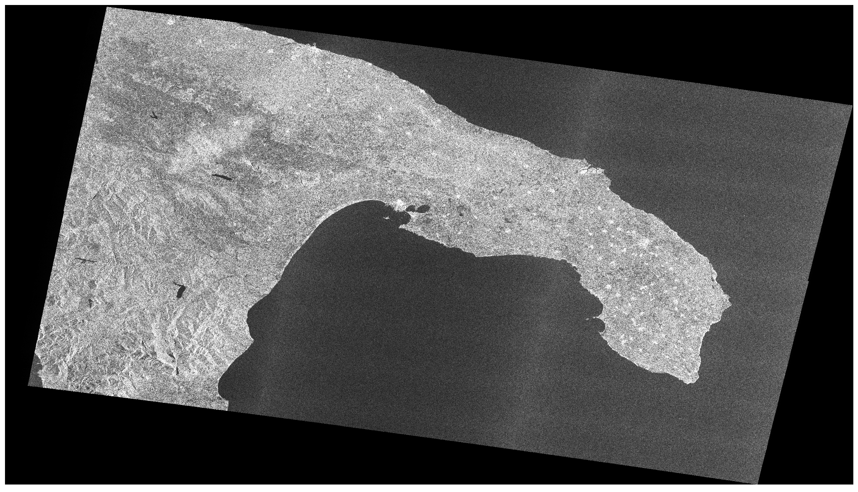
2.1.1. COPERNICUS Sentinel-1 Satellite Data
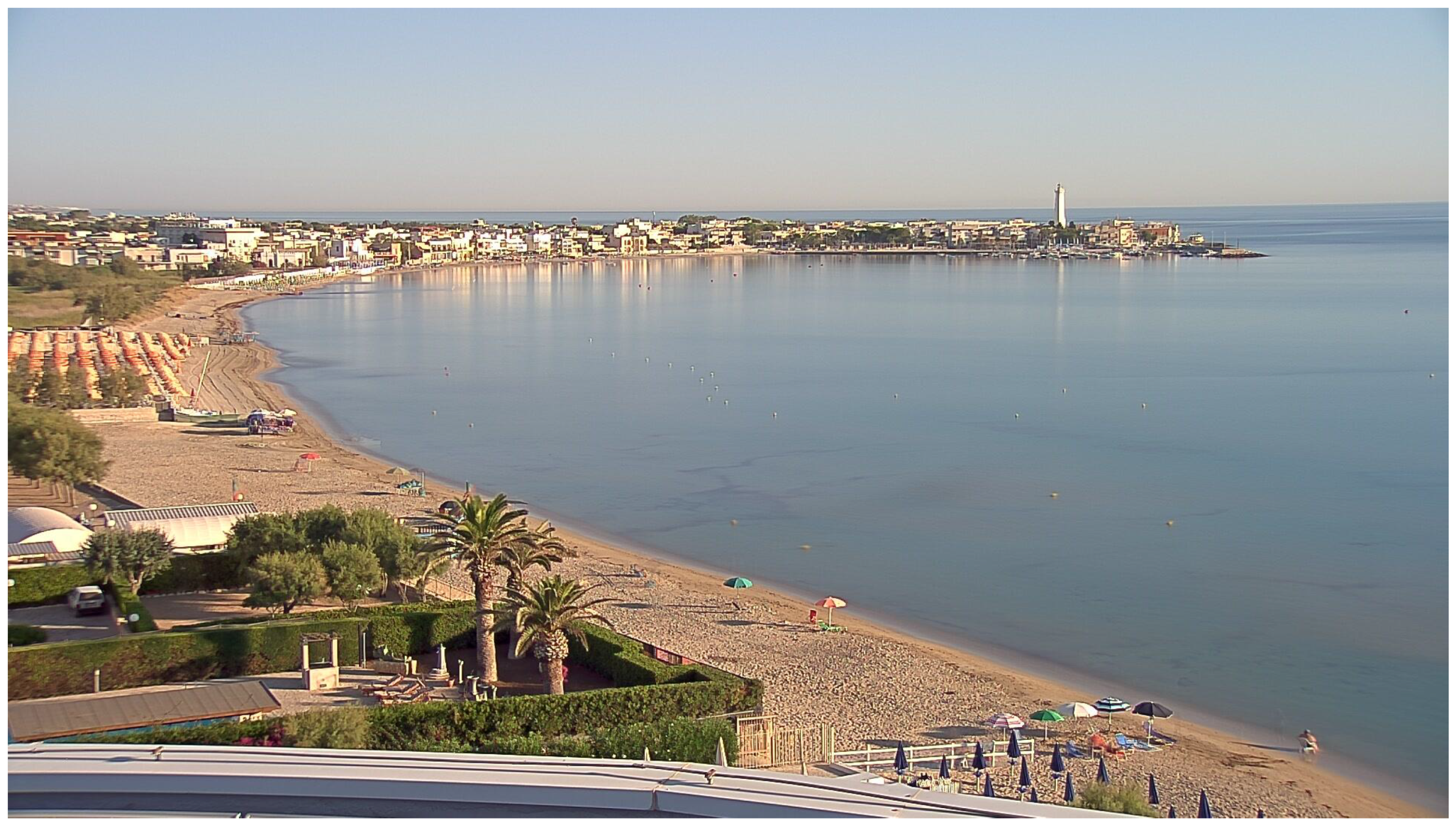
2.1.2. Validation Data
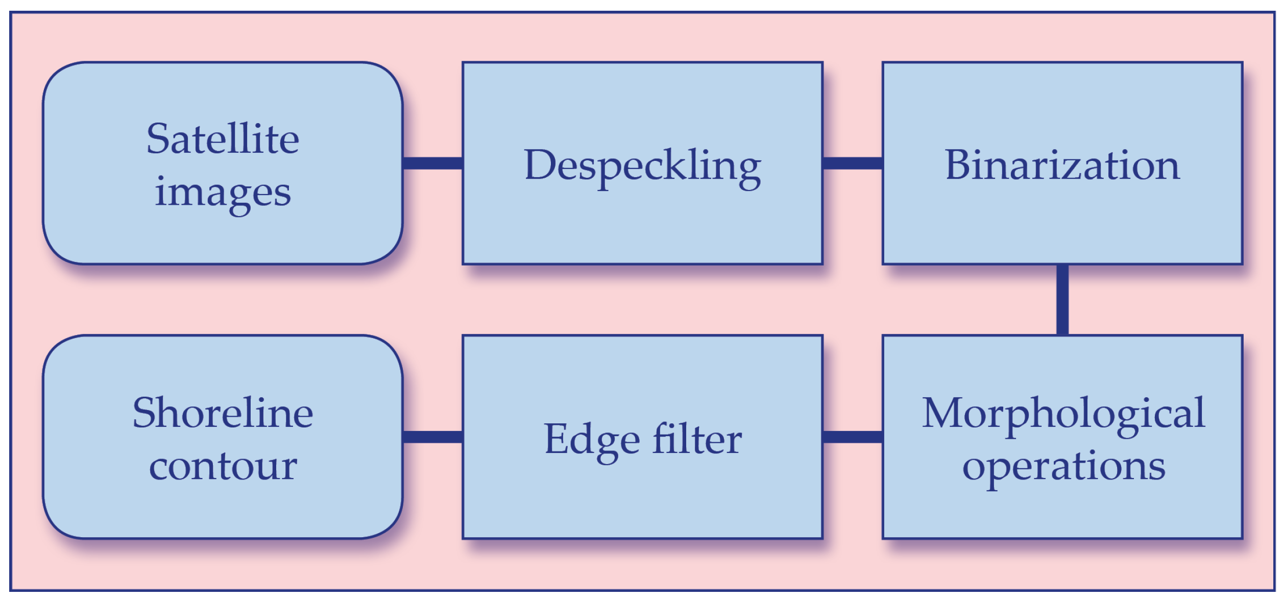
2.2. Methods
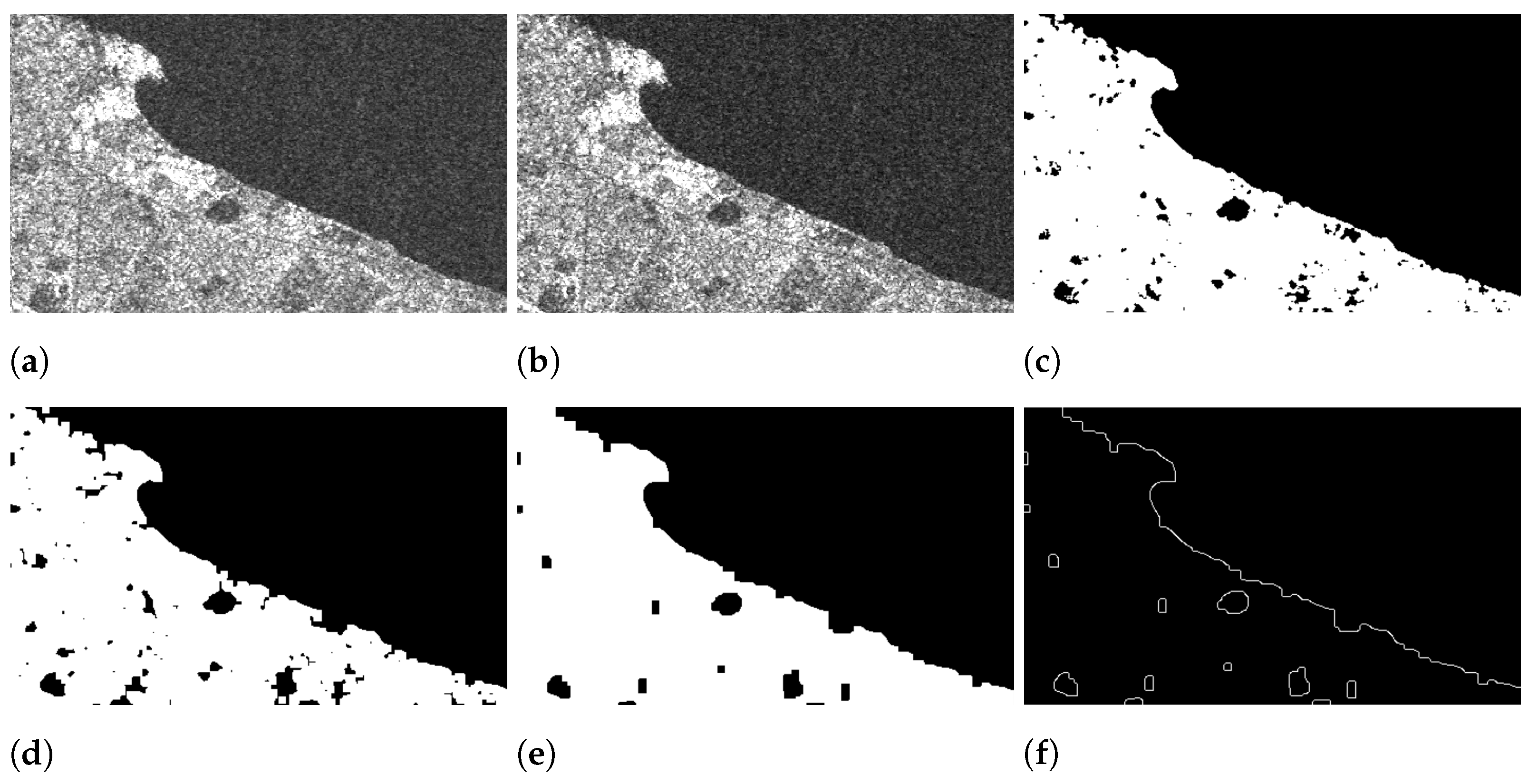
2.2.1. Despeckling
2.2.2. Binarization
2.2.3. Morphological Operation
2.2.4. Canny Edge Detector
3. Results
3.1. Sentinel-1 Retrieved Shoreline
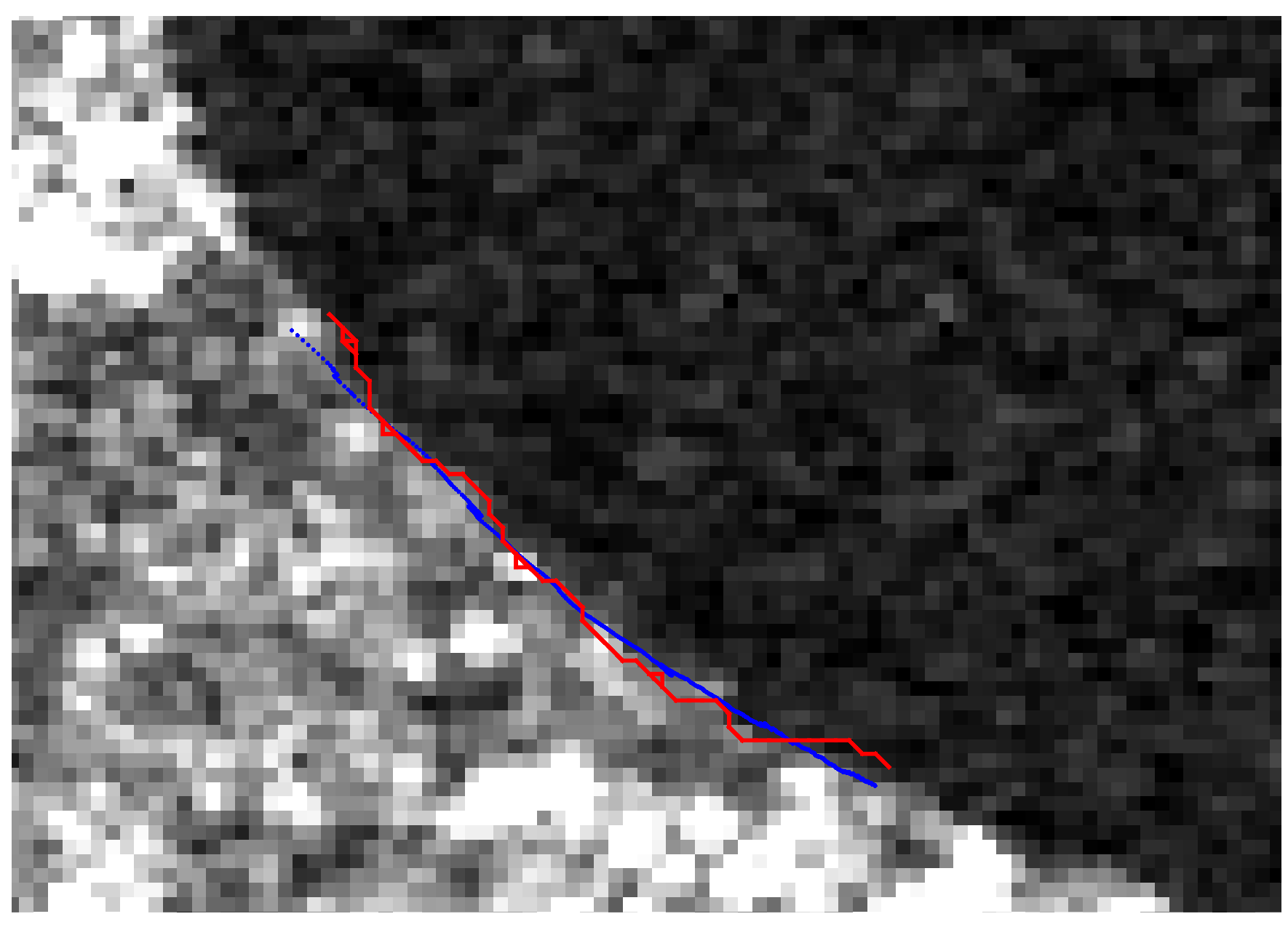
3.2. Shoreline Position Validated against Video Monitoring System-Derived Shoreline
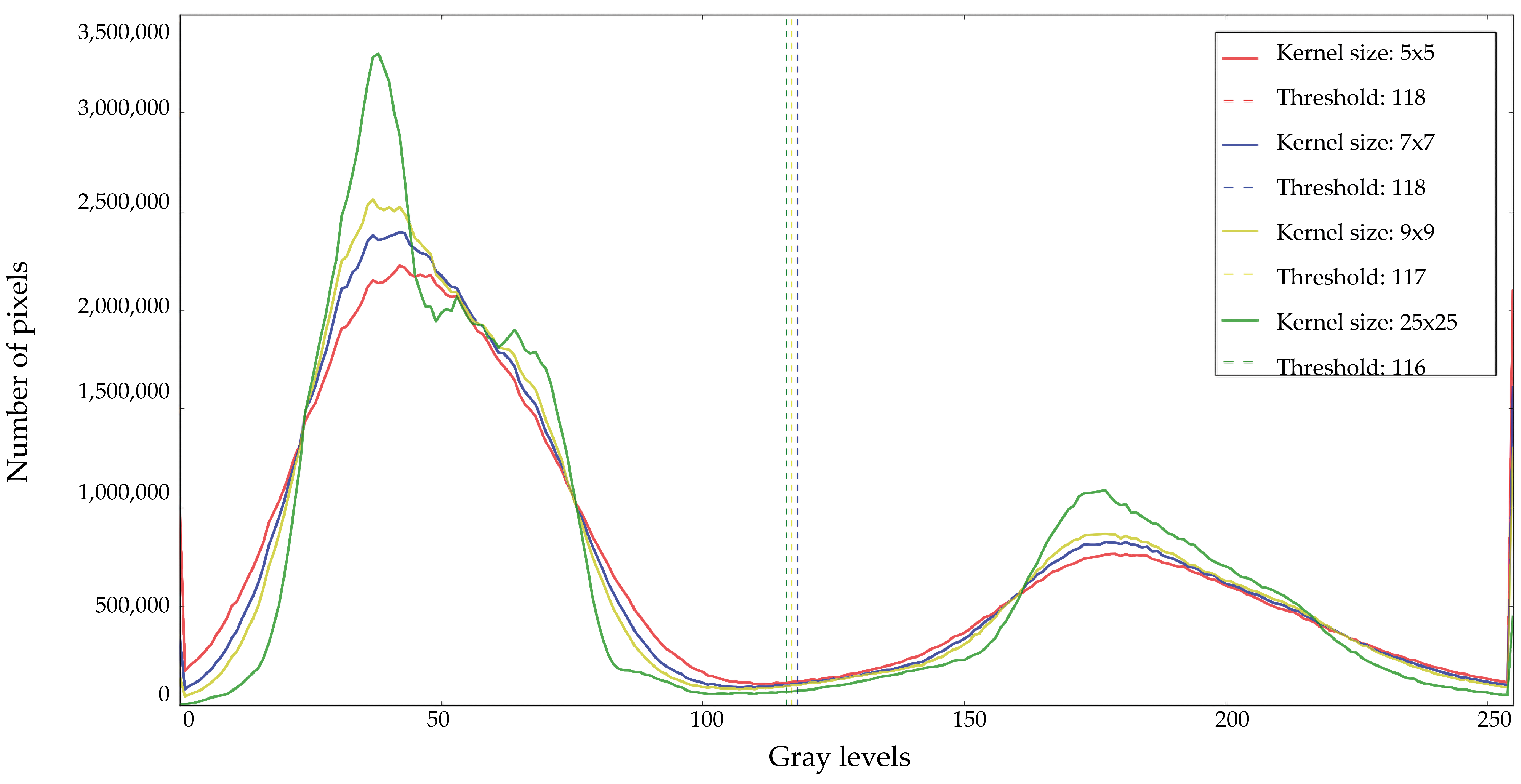
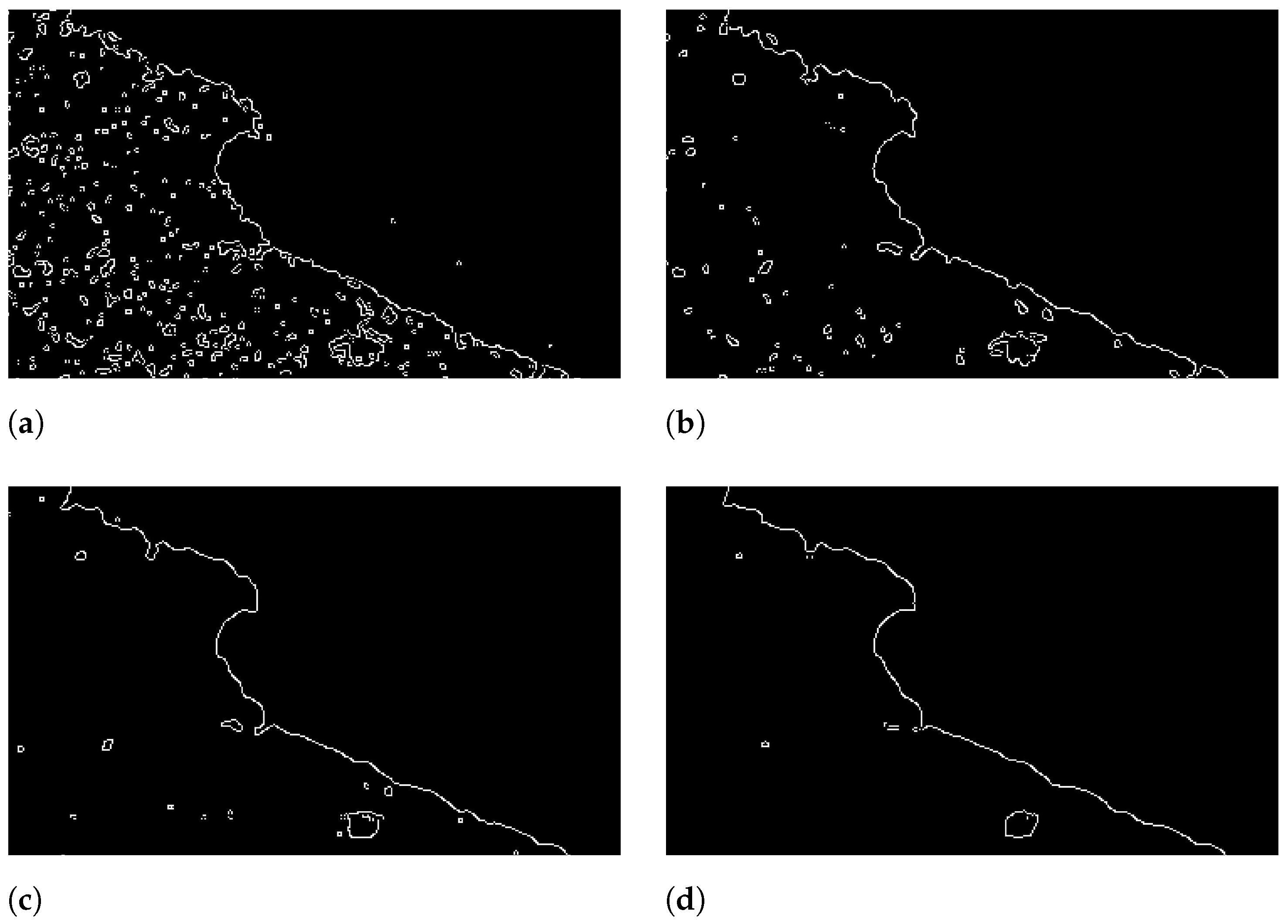
3.3. The Effect of the Despeckling Kernel Size on the Shoreline Position
3.4. Versatility of the Presented Methodology
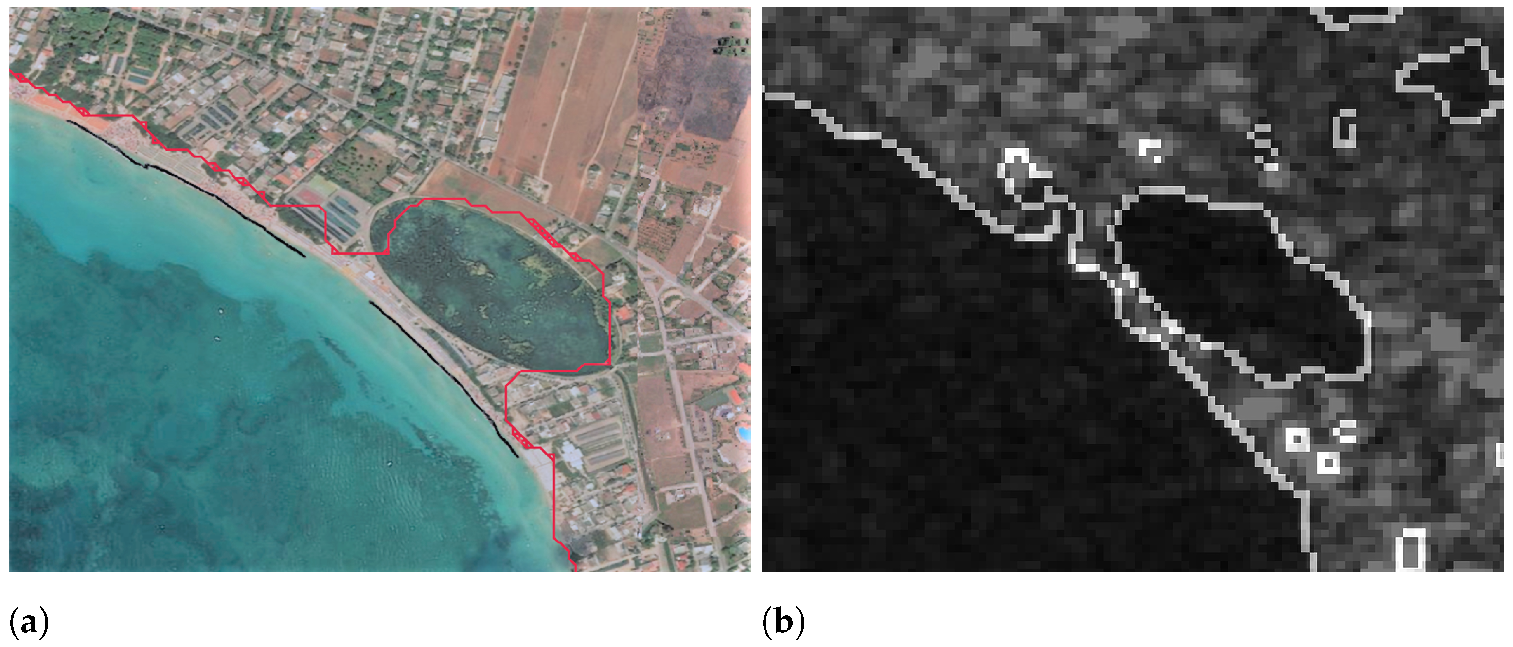
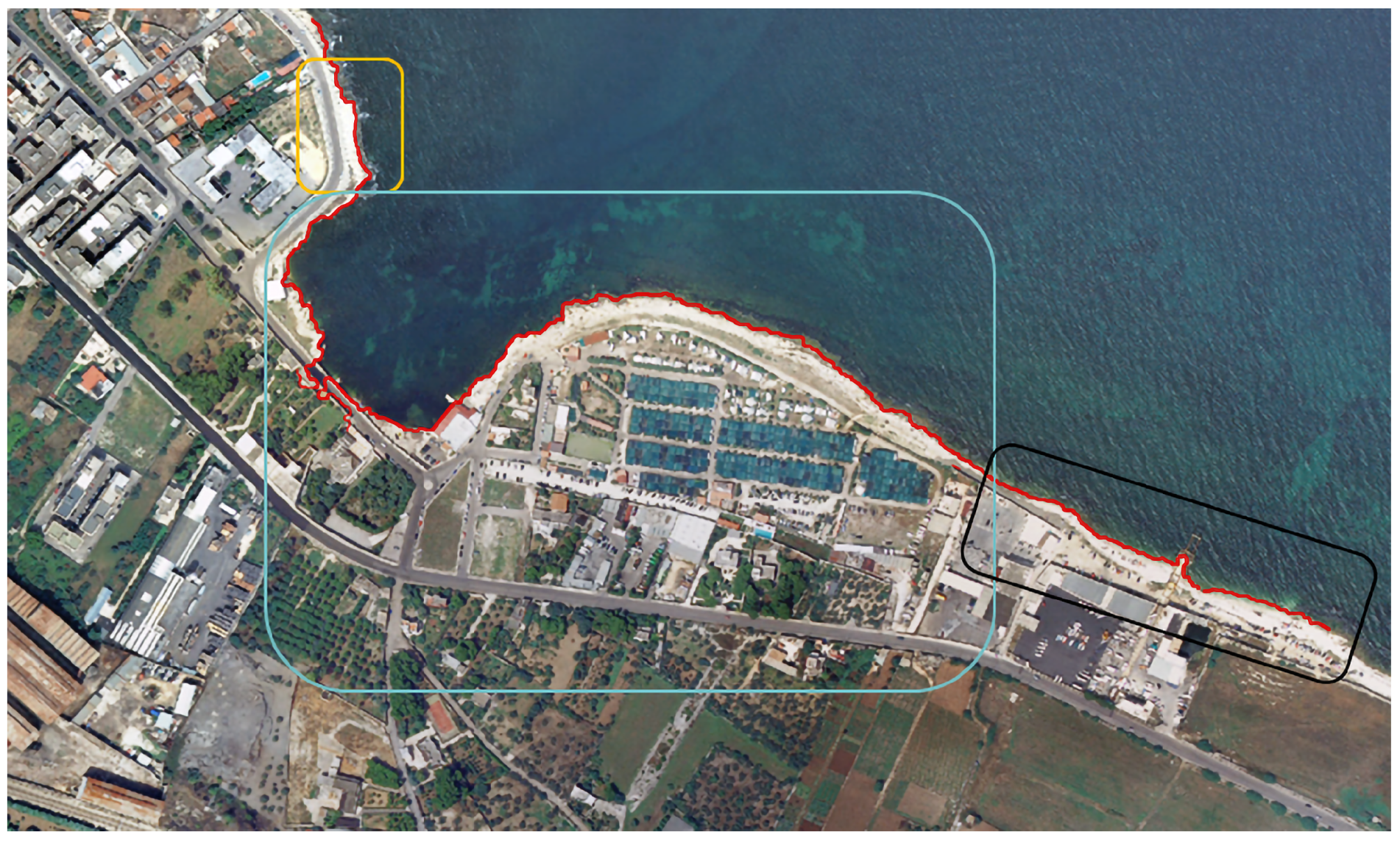
3.4.1. Torre Lapillo
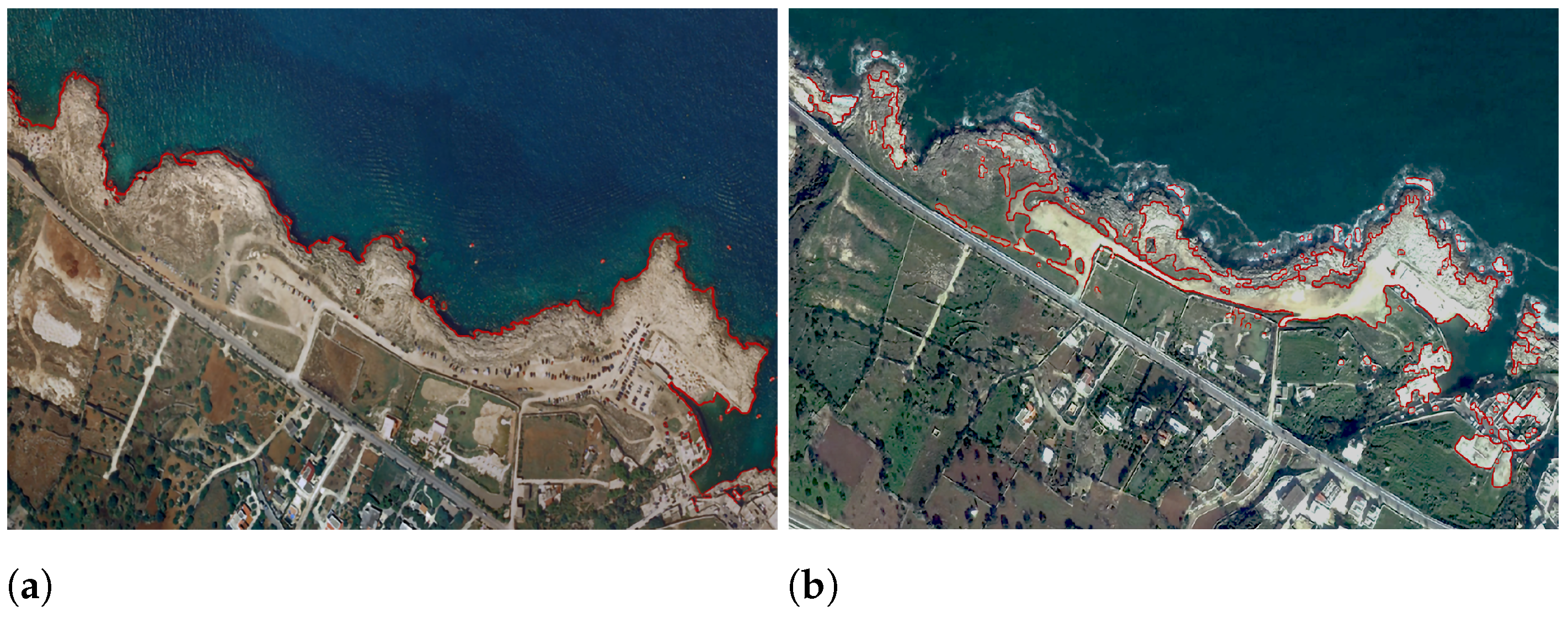
3.4.2. Aerial Images: Giovinazzo
4. Discussion
5. Conclusions
Author Contributions
Funding
Institutional Review Board Statement
Informed Consent Statement
Data Availability Statement
Acknowledgments
Conflicts of Interest
Abbreviations
| ESA | European Space Agency |
| EO | Earth Observation |
| NASA | National Aeronautics and Space Administration |
| PACE | Plankton, Aerosol, Cloud, ocean Ecosystem |
| ERS | European Remote Sensing |
| SAR | Synthetic-Aperture Radar |
| SDS | Satellite Derived Shoreline |
| N-NW | North-North-west |
| E-SE | East-South-east |
| GMES | Global Monitoring for Environment and Security |
| DIAS | Data and Information Access Services |
| IW | Interferometric Wide |
| VH | vertical-horizontal |
| HV | horizontal-vertical |
| VV | vertical-vertical |
| L1D | Level-1 Data |
| GRD | ground range detected |
| SLC | single look complex |
| FR | full resolution |
| HR | high resolution |
| MR | medium resolution |
| OpenCv | Python Open Source Computer Vision |
| EDT | Edge Detection Technique |
| VDS | Video-Derived Shoreline |
| GLIMR | Geosynchronous Littoral Imaging and Monitoring Radiometer |
References
- Gornitz, V. Global coastal hazards from future sea level rise. Palaeogeogr. Palaeoclimatol. Palaeoecol. 1991, 89, 379–398. [Google Scholar] [CrossRef]
- Harley, C.D.; Randall Hughes, A.; Hultgren, K.M.; Miner, B.G.; Sorte, C.J.; Thornber, C.S.; Rodriguez, L.F.; Tomanek, L.; Williams, S.L. The impacts of climate change in coastal marine systems. Ecol. Lett. 2006, 9, 228–241. [Google Scholar] [CrossRef] [Green Version]
- Androulidakis, Y.S.; Kombiadou, K.D.; Makris, C.V.; Baltikas, V.N.; Krestenitis, Y.N. Storm surges in the Mediterranean Sea: Variability and trends under future climatic conditions. Dyn. Atmos. Ocean. 2015, 71, 56–82. [Google Scholar] [CrossRef]
- Saye, S.E.; Van der Wal, D.; Pye, K.; Blott, S.J. Beach–dune morphological relationships and erosion/accretion: An investigation at five sites in England and Wales using LIDAR data. Geomorphology 2005, 72, 128–155. [Google Scholar] [CrossRef]
- Duarte, C.M.; Losada, I.J.; Hendriks, I.E.; Mazarrasa, I.; Marbà, N. The role of coastal plant communities for climate change mitigation and adaptation. Nat. Clim. Chang. 2013, 3, 961. [Google Scholar] [CrossRef] [Green Version]
- Alongi, D.M. Mangrove forests: Resilience, protection from tsunamis, and responses to global climate change. Estuar. Coast. Shelf Sci. 2008, 76, 1–13. [Google Scholar] [CrossRef]
- Antonioli, F.; Anzidei, M.; Amorosi, A.; Presti, V.L.; Mastronuzzi, G.; Deiana, G.; De Falco, G.; Fontana, A.; Fontolan, G.; Lisco, S.; et al. Sea-level rise and potential drowning of the Italian coastal plains: Flooding risk scenarios for 2100. Quat. Sci. Rev. 2017, 158, 29–43. [Google Scholar] [CrossRef] [Green Version]
- Bruno, M.F.; Saponieri, A.; Molfetta, M.G.; Damiani, L. The DPSIR Approach for Coastal Risk Assessment under Climate Change at Regional Scale: The Case of Apulian Coast (Italy). J. Mar. Sci. Eng. 2020, 8, 531. [Google Scholar] [CrossRef]
- Maiolo, M.; Mel, R.A.; Sinopoli, S. A Stepwise Approach to Beach Restoration at Calabaia Beach. Water 2020, 12, 2677. [Google Scholar] [CrossRef]
- Sinay, L.; Carter, R. Climate change adaptation options for coastal communities and local governments. Climate 2020, 8, 7. [Google Scholar] [CrossRef] [Green Version]
- Temmerman, S.; Meire, P.; Bouma, T.J.; Herman, P.M.; Ysebaert, T.; De Vriend, H.J. Ecosystem-based coastal defence in the face of global change. Nature 2013, 504, 79–83. [Google Scholar] [CrossRef]
- Young, A.P.; Ashford, S.A. Application of airborne LIDAR for seacliff volumetric change and beach-sediment budget contributions. J. Coast. Res. 2006, 22, 307–318. [Google Scholar] [CrossRef] [Green Version]
- Stive, M.J.; Aarninkhof, S.G.; Hamm, L.; Hanson, H.; Larson, M.; Wijnberg, K.M.; Nicholls, R.J.; Capobianco, M. Variability of shore and shoreline evolution. Coast. Eng. 2002, 47, 211–235. [Google Scholar] [CrossRef]
- Anfuso, G.; Pranzini, E.; Vitale, G. An integrated approach to coastal erosion problems in northern Tuscany (Italy): Littoral morphological evolution and cell distribution. Geomorphology 2011, 129, 204–214. [Google Scholar] [CrossRef]
- Dolan, R.; Hayden, B.P.; May, P.; May, S. The reliability of shoreline change measurements from aerial photographs. Shore Beach 1980, 48, 22–29. [Google Scholar]
- Boak, E.H.; Turner, I.L. Shoreline definition and detection: A review. J. Coast. Res. 2005, 21, 688–703. [Google Scholar] [CrossRef] [Green Version]
- Dolan, R.; Hayden, B.; Heywood, J. Analysis of coastal erosion and storm surge hazards. Coast. Eng. 1978, 2, 41–53. [Google Scholar] [CrossRef]
- Cooper, J.A.G.; Navas, F. Natural bathymetric change as a control on century-scale shoreline behavior. Geology 2004, 32, 513–516. [Google Scholar] [CrossRef]
- White, S.A.; Wang, Y. Utilizing DEMs derived from LIDAR data to analyze morphologic change in the North Carolina coastline. Remote Sens. Environ. 2003, 85, 39–47. [Google Scholar] [CrossRef]
- Nitti, D.O.; Nutricato, R.; Lorusso, R.; Lombardi, N.; Bovenga, F.; Bruno, M.F.; Chiaradia, M.T.; Milillo, G. On the geolocation accuracy of COSMO-SkyMed products. In Proceedings of the SAR Image Analysis, Modeling, and Techniques XV—International Society for Optics and Photonics, Toulouse, France, 23–24 September 2015; Volume 9642, p. 96420D. [Google Scholar]
- Luijendijk, A.; Hagenaars, G.; Ranasinghe, R.; Baart, F.; Donchyts, G.; Aarninkhof, S. The state of the world’s beaches. Sci. Rep. 2018, 8, 1–11. [Google Scholar] [CrossRef]
- Vos, K.; Splinter, K.D.; Harley, M.D.; Simmons, J.A.; Turner, I.L. CoastSat: A Google Earth Engine-enabled Python toolkit to extract shorelines from publicly available satellite imagery. Environ. Model. Softw. 2019, 122, 104528. [Google Scholar] [CrossRef]
- Vos, K.; Harley, M.D.; Splinter, K.D.; Simmons, J.A.; Turner, I.L. Sub-annual to multi-decadal shoreline variability from publicly available satellite imagery. Coast. Eng. 2019, 150, 160–174. [Google Scholar] [CrossRef]
- García-Rubio, G.; Huntley, D.; Russell, P. Evaluating shoreline identification using optical satellite images. Mar. Geol. 2015, 359, 96–105. [Google Scholar] [CrossRef] [Green Version]
- Wei, X.; Zheng, W.; Xi, C.; Shang, S. Shoreline Extraction in SAR Image Based on Advanced Geometric Active Contour Model. Remote Sens. 2021, 13, 642. [Google Scholar] [CrossRef]
- Zollini, S.; Alicandro, M.; Cuevas-González, M.; Baiocchi, V.; Dominici, D.; Buscema, P.M. Shoreline extraction based on an active connection matrix (ACM) image enhancement strategy. J. Mar. Sci. Eng. 2020, 8, 9. [Google Scholar] [CrossRef] [Green Version]
- Pardo-Pascual, J.E.; Almonacid-Caballer, J.; Ruiz, L.A.; Palomar-Vázquez, J. Automatic extraction of shorelines from Landsat TM and ETM+ multi-temporal images with subpixel precision. Remote Sens. Environ. 2012, 123, 1–11. [Google Scholar] [CrossRef] [Green Version]
- Valentini, N.; Saponieri, A.; Damiani, L. A new video monitoring system in support of Coastal Zone Management at Apulia Region, Italy. Ocean. Coast. Manag. 2017, 142, 122–135. [Google Scholar] [CrossRef]
- Damiani, L.; Molfetta, M.G. A video based technique for shoreline monitoring in Alimini (LE). Coastlab08 2008, 8, 153–156. [Google Scholar]
- Splinter, K.D.; Harley, M.D.; Turner, I.L. Remote sensing is changing our view of the coast: Insights from 40 years of monitoring at Narrabeen-Collaroy, Australia. Remote Sens. 2018, 10, 1744. [Google Scholar] [CrossRef] [Green Version]
- Holman, R.A.; Stanley, J. The history and technical capabilities of Argus. Coast. Eng. 2007, 54, 477–491. [Google Scholar] [CrossRef]
- Morton, R.A.; Leach, M.P.; Paine, J.G.; Cardoza, M.A. Monitoring beach changes using GPS surveying techniques. J. Coast. Res. 1993, 9, 702–720. [Google Scholar]
- Medellín, G.; Torres-Freyermuth, A.; Tomasicchio, G.R.; Francone, A.; Tereszkiewicz, P.A.; Lusito, L.; Palemón-Arcos, L.; López, J. Field and Numerical Study of Resistance and Resilience on a Sea Breeze Dominated Beach in Yucatan (Mexico). Water 2018, 10, 1806. [Google Scholar] [CrossRef] [Green Version]
- Tomasicchio, G.R.; Francone, A.; Simmonds, D.J.; D’Alessandro, F.; Frega, F. Prediction of Shoreline Evolution. Reliability of a General Model for the Mixed Beach Case. J. Mar. Sci. Eng. 2020, 8, 361. [Google Scholar] [CrossRef]
- Dellepiane, S.; De Laurentiis, R.; Giordano, F. Coastline extraction from SAR images and a method for the evaluation of the coastline precision. Pattern Recognit. Lett. 2004, 25, 1461–1470. [Google Scholar] [CrossRef]
- Valentini, N.; Saponieri, A.; Molfetta, M.G.; Damiani, L. New algorithms for shoreline monitoring from coastal video systems. Earth Sci. Inform. 2017, 10, 495–506. [Google Scholar] [CrossRef]
- Aarninkhof, S.G.; Turner, I.L.; Dronkers, T.D.; Caljouw, M.; Nipius, L. A video-based technique for mapping intertidal beach bathymetry. Coast. Eng. 2003, 49, 275–289. [Google Scholar] [CrossRef]
- Aagaard, T.; Holm, J. Digitization of wave run-up using video records. J. Coast. Res. 1989, 5, 547–551. [Google Scholar]
- Vousdoukas, M.I.; Wziatek, D.; Almeida, L.P. Coastal vulnerability assessment based on video wave run-up observations at a mesotidal, steep-sloped beach. Ocean Dyn. 2012, 62, 123–137. [Google Scholar] [CrossRef]
- Hoitink, A.; Wang, Z.; Vermeulen, B.; Huismans, Y.; Kästner, K. Tidal controls on river delta morphology. Nat. Geosci. 2017, 10, 637–645. [Google Scholar] [CrossRef] [Green Version]
- Moulton, M.; Elgar, S.; Raubenheimer, B.; Warner, J.C.; Kumar, N. Rip currents and alongshore flows in single channels dredged in the surf zone. J. Geophys. Res. Ocean. 2017, 122, 3799–3816. [Google Scholar] [CrossRef]
- Medina, R.; Marino-Tapia, I.; Osorio, A.; Davidson, M.; Martin, F. Management of dynamic navigational channels using video techniques. Coast. Eng. 2007, 54, 523–537. [Google Scholar] [CrossRef]
- Martínez, A.; Eckert, E.M.; Artois, T.; Careddu, G.; Casu, M.; Curini-Galletti, M.; Gazale, V.; Gobert, S.; Ivanenko, V.N.; Jondelius, U.; et al. Human access impacts biodiversity of microscopic animals in sandy beaches. Commun. Biol. 2020, 3, 1–9. [Google Scholar] [CrossRef] [Green Version]
- Machado, P.M.; Suciu, M.C.; Costa, L.L.; Tavares, D.C.; Zalmon, I.R. Tourism impacts on benthic communities of sandy beaches. Mar. Ecol. 2017, 38, e12440. [Google Scholar] [CrossRef]
- Gons, H.J.; Rijkeboer, M.; Ruddick, K.G. A chlorophyll-retrieval algorithm for satellite imagery (Medium Resolution Imaging Spectrometer) of inland and coastal waters. J. Plankton Res. 2002, 24, 947–951. [Google Scholar] [CrossRef] [Green Version]
- Chassot, E.; Bonhommeau, S.; Reygondeau, G.; Nieto, K.; Polovina, J.J.; Huret, M.; Dulvy, N.K.; Demarcq, H. Satellite remote sensing for an ecosystem approach to fisheries management. ICES J. Mar. Sci. 2011, 68, 651–666. [Google Scholar] [CrossRef] [Green Version]
- Emery, W.; Matthews, D.; Baldwin, D. Mapping surface coastal currents with satellite imagery and altimetry. In Proceedings of the USA-Baltic Internation Symposium, Klaipeda, Lithuania, 15–17 June 2004; pp. 1–5. [Google Scholar]
- Liu, H.; Jezek, K. Automated extraction of coastline from satellite imagery by integrating Canny edge detection and locally adaptive thresholding methods. Int. J. Remote Sens. 2004, 25, 937–958. [Google Scholar] [CrossRef]
- Lee, J.S.; Jurkevich, I. Coastline detection and tracing in SAR images. IEEE Trans. Geosci. Remote Sens. 1990, 28, 662–668. [Google Scholar]
- Mason, D.C.; Davenport, I.J. Accurate and efficient determination of the shoreline in ERS-1 SAR images. IEEE Trans. Geosci. Remote Sens. 1996, 34, 1243–1253. [Google Scholar] [CrossRef]
- Niedermeier, A.; Romaneessen, E.; Lehner, S. Detection of coastlines in SAR images using wavelet methods. IEEE Trans. Geosci. Remote Sens. 2000, 38, 2270–2281. [Google Scholar] [CrossRef]
- Mallat, S.; Zhong, S. Characterization of signals from multiscale edges. IEEE Trans. Pattern Anal. Mach. Intell. 1992, 14, 710–732. [Google Scholar] [CrossRef] [Green Version]
- Mallat, S.; Hwang, W.L. Singularity detection and processing with wavelets. IEEE Trans. Inf. Theory 1992, 38, 617–643. [Google Scholar] [CrossRef]
- Otsu, N. A threshold selection method from gray-level histograms. IEEE Trans. Syst. Man Cybern. 1979, 9, 62–66. [Google Scholar] [CrossRef] [Green Version]
- Padmasini, N.; Umamaheswari, R.; Sikkandar, M.Y. State-of-the-Art of Level-Set Methods in Segmentation and Registration of Spectral Domain Optical Coherence Tomographic Retinal Images. In Soft Computing Based Medical Image Analysis; Academic Press: Cambridge, MA, USA, 2018; pp. 163–181. [Google Scholar]
- Meta, A.; Prats, P.; Steinbrecher, U.; Mittermayer, J.; Scheiber, R. TerraSAR-X TOPSAR and ScanSAR comparison. In Proceedings of the Synthetic Aperture Radar (EUSAR), Friedrichshafen, Germany, 2–5 June 2008; pp. 1–4. [Google Scholar]
- Gulácsi, A.; Kovács, F. Sentinel-1-imagery-based high-resolution water cover detection on wetlands, Aided by Google Earth Engine. Remote Sens. 2020, 12, 1614. [Google Scholar] [CrossRef]
- Xing, L.; Tang, X.; Wang, H.; Fan, W.; Wang, G. Monitoring monthly surface water dynamics of Dongting Lake using Sentinel-1 data at 10 m. PeerJ 2018, 6, e4992. [Google Scholar] [CrossRef] [PubMed]
- Brisco, B. Mapping and monitoring surface water and wetlands with synthetic aperture radar. Remote Sens. Wetlands Appl. Adv. 2015, 119–136. [Google Scholar] [CrossRef]
- Valentini, N.; Damiani, L.; Molfetta, M.G.; Saponieri, A. New coastal video-monitoring system achievement and development. Coast. Eng. Proc. 2017, 1, 11. [Google Scholar] [CrossRef]
- Bradski, G.; Kaehler, A. OpenCV. Dr. Dobb’s Journal of Software Tools. 2000. Available online: https://www.scirp.org/(S(351jmbntvnsjt1aadkposzje))/reference/ReferencesPapers.aspx?ReferenceID=1692176 (accessed on 26 May 2021).
- Van der Walt, S.; Schönberger, J.L.; Nunez-Iglesias, J.; Boulogne, F.; Warner, J.D.; Yager, N.; Gouillart, E.; Yu, T. scikit-image: Image processing in Python. PeerJ 2014, 2, e453. [Google Scholar] [CrossRef]
- Gagnon, L.; Jouan, A. Speckle filtering of SAR images: A comparative study between complex-wavelet-based and standard filters. In Proceedings of the I. S. Photonics, Wavelet Applications in Signal and Image Processing V, San Diego, CA, USA, 27 July–1 August 1997; Volume 3169, pp. 80–92. [Google Scholar]
- Rajamani, A.; Krishnaveni, V. Performance analysis survey of various SAR image despeckling techniques. Int. J. Comput. Appl. 2014, 90. [Google Scholar] [CrossRef] [Green Version]
- De Vries, F. Speckle Reduction in SAR Imagery by Various Multi-Look Techniques; Technical Report; Fysich en Elektronisch Lab TNO: The Hague, The Netherlands, 1998. [Google Scholar]
- Huang, T.; Yang, G.J.T.G.Y.; Tang, G. A fast two-dimensional median filtering algorithm. IEEE Trans. Acoust. Speech Signal Process. 1979, 27, 13–18. [Google Scholar] [CrossRef] [Green Version]
- Kuan, D.T.; Sawchuk, A.A.; Strand, T.C.; Chavel, P. Adaptive noise smoothing filter for images with signal-dependent noise. IEEE Trans. Pattern Anal. Mach. Intell. 1985, 2, 165–177. [Google Scholar] [CrossRef]
- Frost, V.S.; Stiles, J.A.; Shanmugan, K.S.; Holtzman, J.C. A model for radar images and its application to adaptive digital filtering of multiplicative noise. IEEE Trans. Pattern Anal. Mach. Intell. 1982, 2, 157–166. [Google Scholar] [CrossRef] [PubMed]
- Lopes, A.; Nezry, E.; Touzi, R.; Laur, H. Structure detection and statistical adaptive speckle filtering in SAR images. Int. J. Remote Sens. 1993, 14, 1735–1758. [Google Scholar] [CrossRef]
- Saxena, N.; Rathore, N. A review on speckle noise filtering techniques for SAR images. Int. J. Adv. Res. Comput. Sci. Electron. Eng. (IJARCSEE) 2013, 2, 243. [Google Scholar]
- Modava, M.; Akbarizadeh, G. Coastline extraction from SAR images using spatial fuzzy clustering and the active contour method. Int. J. Remote Sens. 2017, 38, 355–370. [Google Scholar] [CrossRef]
- Donchyts, G.; Schellekens, J.; Winsemius, H.; Eisemann, E.; Van de Giesen, N. A 30 m resolution surface water mask including estimation of positional and thematic differences using landsat 8, srtm and openstreetmap: A case study in the Murray-Darling Basin, Australia. Remote Sens. 2016, 8, 386. [Google Scholar] [CrossRef] [Green Version]
- Li, W.; Du, Z.; Ling, F.; Zhou, D.; Wang, H.; Gui, Y.; Sun, B.; Zhang, X. A comparison of land surface water mapping using the normalized difference water index from TM, ETM+ and ALI. Remote Sens. 2013, 5, 5530–5549. [Google Scholar] [CrossRef] [Green Version]
- Kittler, J.; Illingworth, J. On threshold selection using clustering criteria. IEEE Trans. Syst. Man Cybern. 1985, 5, 652–655. [Google Scholar] [CrossRef]
- Serra, J.; Soille, P. Mathematical Morphology and Its Applications to Image Processing; Springer: Berlin/Heisenberg, Germany, 2012; Volume 2. [Google Scholar]
- Haralick, R.M.; Sternberg, S.R.; Zhuang, X. Image analysis using mathematical morphology. IEEE Trans. Pattern Anal. Mach. Intell. 1987, 4, 532–550. [Google Scholar] [CrossRef]
- Kasturi, R. Image Analysis Applications; CRC Press: Boca Raton, FL, USA, 1990. [Google Scholar]
- Baets, B.D.; Kerre, E.; Gupta, M. The fundamentals of fuzzy mathematical morphology part 1: Basic concepts. Int. J. Gen. Syst. 1995, 23, 155–171. [Google Scholar] [CrossRef]
- Maini, R.; Aggarwal, H. Study and comparison of various image edge detection techniques. Int. J. Image Process. (IJIP) 2009, 3, 1–11. [Google Scholar]
- Marr, D.; Hildreth, E. Theory of edge detection. Proc. R. Soc. London Ser. Biol. Sci. 1980, 207, 187–217. [Google Scholar]
- Canny, J. A computational approach to edge detection. IEEE Trans. Pattern Anal. Mach. Intell. 1986, 6, 679–698. [Google Scholar] [CrossRef]
- Shrivakshan, G.T.; Chandrasekar, C. A comparison of various edge detection techniques used in image processing. Int. J. Comput. Sci. Issues (IJCSI) 2012, 9, 269. [Google Scholar]
- Pelich, R.; Chini, M.; Hostache, R.; Matgen, P.; López-Martínez, C. Coastline Detection Based on Sentinel-1 Time Series for Ship-and Flood-Monitoring Applications. IEEE Geosci. Remote Sens. Lett. 2020. [Google Scholar] [CrossRef]
- Nolet, C.; Poortinga, A.; Roosjen, P.; Bartholomeus, H.; Ruessink, G. Measuring and modeling the effect of surface moisture on the spectral reflectance of coastal beach sand. PLoS ONE 2014, 9, e112151. [Google Scholar] [CrossRef]
- Almeida, L.P.; de Oliveira, I.E.; Lyra, R.; Dazzi, R.L.S.; Martins, V.G.; da Fontoura Klein, A.H. Coastal Analyst System from Space Imagery Engine (CASSIE): Shoreline management module. Environ. Model. Softw. 2021, 140, 105033. [Google Scholar] [CrossRef]
- Montgomery, J.; Brisco, B.; Chasmer, L.; Devito, K.; Cobbaert, D.; Hopkinson, C. SAR and LiDAR temporal data fusion approaches to boreal wetland ecosystem monitoring. Remote Sens. 2019, 11, 161. [Google Scholar] [CrossRef] [Green Version]
- Lin, C.; Wu, C.C.; Tsogt, K.; Ouyang, Y.C.; Chang, C.I. Effects of atmospheric correction and pansharpening on LULC classification accuracy using WorldView-2 imagery. Inf. Process. Agric. 2015, 2, 25–36. [Google Scholar] [CrossRef] [Green Version]
- Du, P.; Liu, S.; Xia, J.; Zhao, Y. Information fusion techniques for change detection from multi-temporal remote sensing images. Inf. Fusion 2013, 14, 19–27. [Google Scholar] [CrossRef]
- Cenci, L.; Persichillo, M.G.; Disperati, L.; Oliveira, E.R.; Alves, F.L.; Pulvirenti, L.; Rebora, N.; Boni, G.; Phillips, M. Remote sensing for coastal risk reduction purposes: Optical and microwave data fusion for shoreline evolution monitoring and modelling. In Proceedings of the 2015 IEEE International Geoscience and Remote Sensing Symposium (IGARSS), Milan, Italy, 26–31 July 2015; pp. 1417–1420. [Google Scholar]
- Ruiz-Beltran, A.P.; Astorga-Moar, A.; Salles, P.; Appendini, C.M. Short-term shoreline trend detection patterns using SPOT-5 image fusion in the northwest of Yucatan, Mexico. Estuaries Coasts 2019, 42, 1761–1773. [Google Scholar] [CrossRef]
- Billa, L.; Pradhan, B. Semi-automated procedures for shoreline extraction using single RADARSAT-1 SAR image. Estuarine Coast. Shelf Sci. 2011, 95, 395–400. [Google Scholar]
- Alicandro, M.; Baiocchi, V.; Brigante, R.; Radicioni, F. Automatic shoreline detection from eight-band VHR satellite imagery. J. Mar. Sci. Eng. 2019, 7, 459. [Google Scholar] [CrossRef] [Green Version]
- Palazzo, F.; Latini, D.; Baiocchi, V.; Del Frate, F.; Giannone, F.; Dominici, D.; Remondiere, S. An application of COSMO-Sky Med to coastal erosion studies. Eur. J. Remote Sens. 2012, 45, 361–370. [Google Scholar] [CrossRef] [Green Version]


| Date | Time Sentinel-1 | Time Webcam | Minimum Distance [m] | Maximum Distance [m] | RMSE [m] |
|---|---|---|---|---|---|
| 19 February 2017 | 04:55 | 05:00 | 0.001 | 23.381 | 8.373 |
| 27 March 2017 | 04:55 | 05:00 | 0.026 | 36.172 | 9.601 |
| 15 May 2017 | 16:40 | 17:00 | 2.401 | 31.482 | 15.329 |
| 26 May 2017 | 04:55 | 05:00 | 0.005 | 35.565 | 13.065 |
| 27 May 2017 | 16:40 | 16:30 | 0.008 | 31.010 | 11.285 |
| 7 June 2017 | 04:55 | 05:00 | 0.012 | 18.638 | 6.132 |
| 8 June 2017 | 16:40 | 17:00 | 0.002 | 27.671 | 10.061 |
| 6 October 2017 | 16:40 | 17:00 | 11.108 | 44.737 | 23.206 |
| 18 October 2017 | 16:40 | 17:00 | 0.002 | 33.328 | 12.615 |
| 30 October 2017 | 16:40 | 17:00 | 0.706 | 37.797 | 14.049 |
| 16 December 2017 | 04:55 | 05:00 | 0.045 | 32.315 | 13.454 |
| average | 12.479 |
Publisher’s Note: MDPI stays neutral with regard to jurisdictional claims in published maps and institutional affiliations. |
© 2021 by the authors. Licensee MDPI, Basel, Switzerland. This article is an open access article distributed under the terms and conditions of the Creative Commons Attribution (CC BY) license (https://creativecommons.org/licenses/by/4.0/).
Share and Cite
Spinosa, A.; Ziemba, A.; Saponieri, A.; Damiani, L.; El Serafy, G. Remote Sensing-Based Automatic Detection of Shoreline Position: A Case Study in Apulia Region. J. Mar. Sci. Eng. 2021, 9, 575. https://doi.org/10.3390/jmse9060575
Spinosa A, Ziemba A, Saponieri A, Damiani L, El Serafy G. Remote Sensing-Based Automatic Detection of Shoreline Position: A Case Study in Apulia Region. Journal of Marine Science and Engineering. 2021; 9(6):575. https://doi.org/10.3390/jmse9060575
Chicago/Turabian StyleSpinosa, Anna, Alex Ziemba, Alessandra Saponieri, Leonardo Damiani, and Ghada El Serafy. 2021. "Remote Sensing-Based Automatic Detection of Shoreline Position: A Case Study in Apulia Region" Journal of Marine Science and Engineering 9, no. 6: 575. https://doi.org/10.3390/jmse9060575