
Numerical Analysis of Storm Surges on Canada’s Western Arctic Coastline


Abstract
:1. Introduction
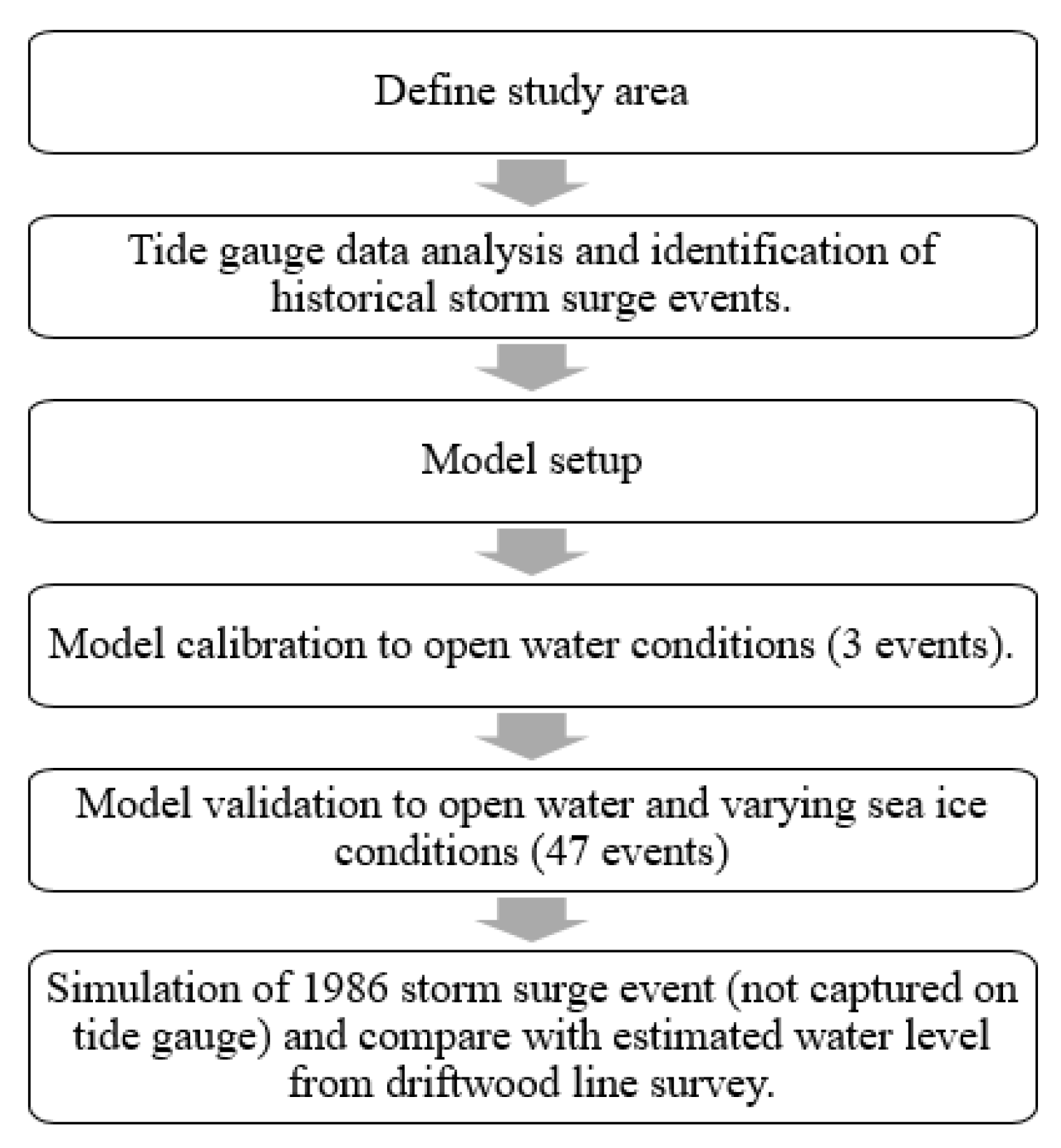
2. Methodology
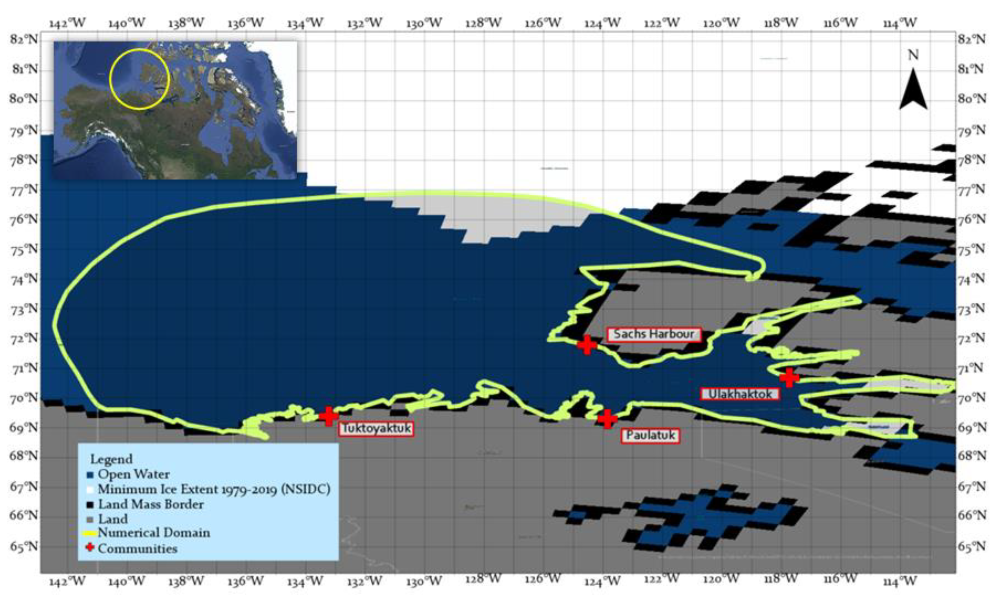
3. Study Area
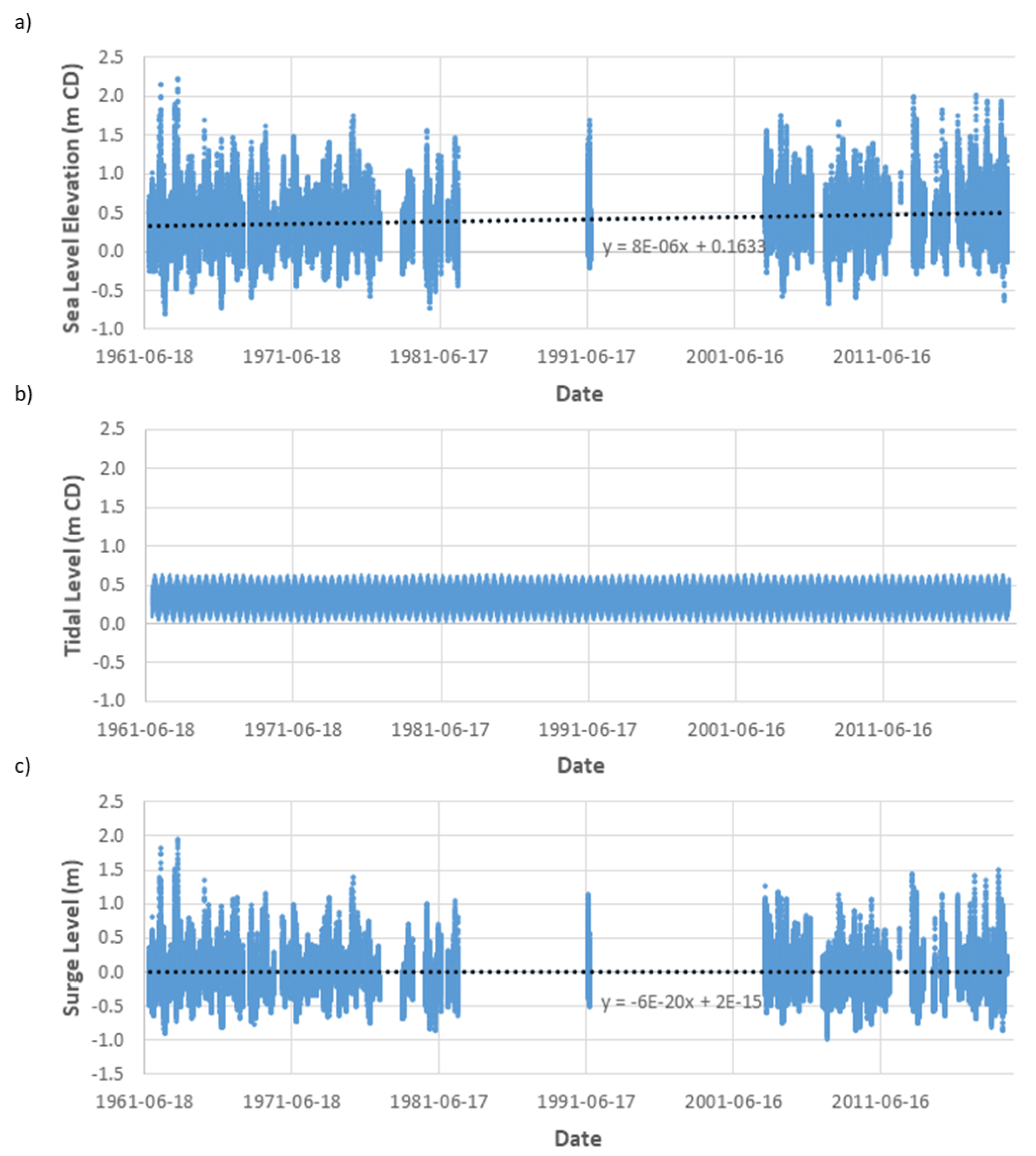
4. Tide Gauge Analysis
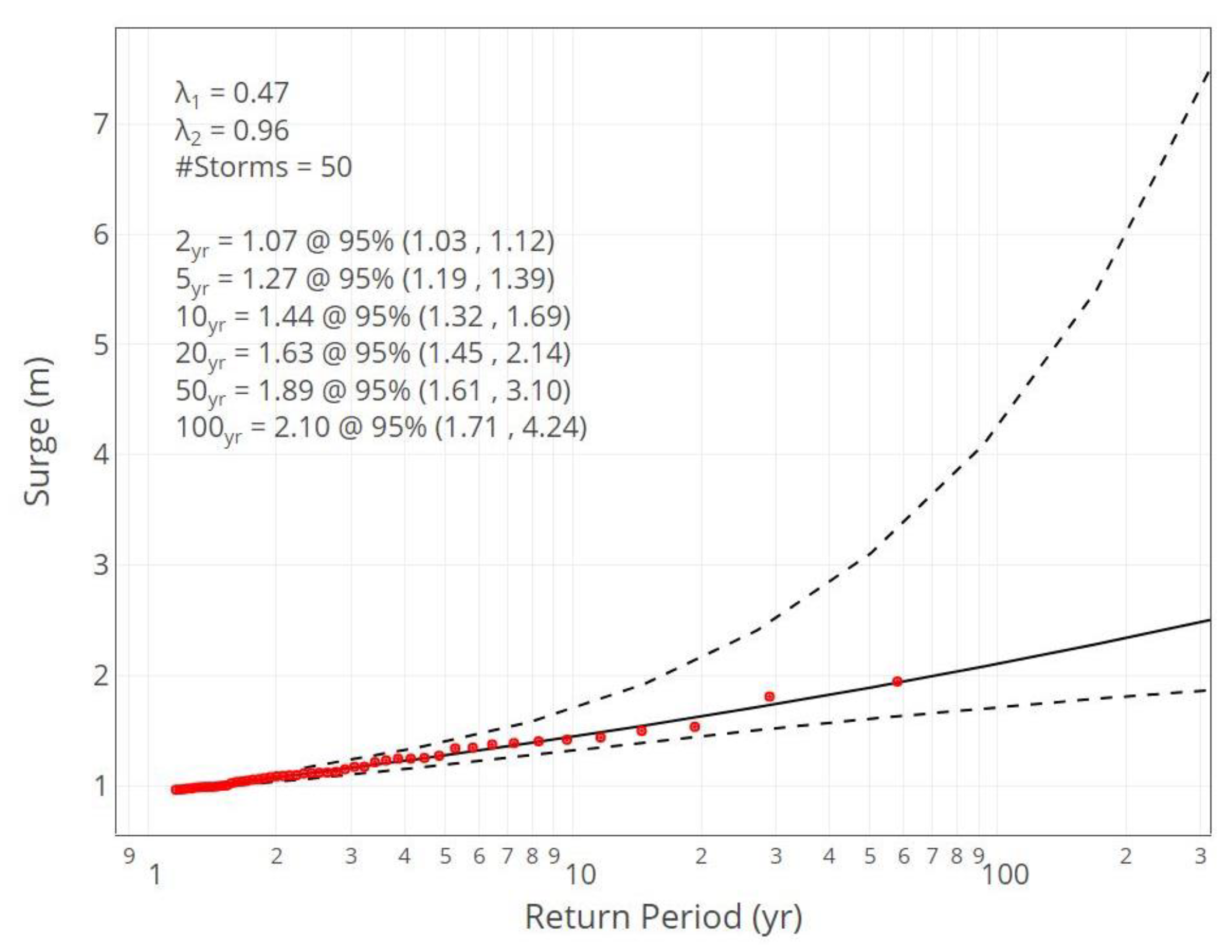
Identification of Storm Surge Events and Extreme Value Analysis
5. Model Setup
5.1. Reanalysis Dataset
5.2. Effect of Ice Presence on Storm Surges
5.3. Sensitivity Study
6. Results
6.1. Calibration and Validation
6.2. Hindcast of the 23 August 1986 Storm Surge Event
7. Discussion
7.1. Quality of the ERA5 Dataset
7.2. Quality of Historic Tide Gauge Records and Impacts on Uncertainty
7.3. Effects of Sea Ice Conditions on Storm Surges
7.4. Limitations and Research Needs
8. Conclusions
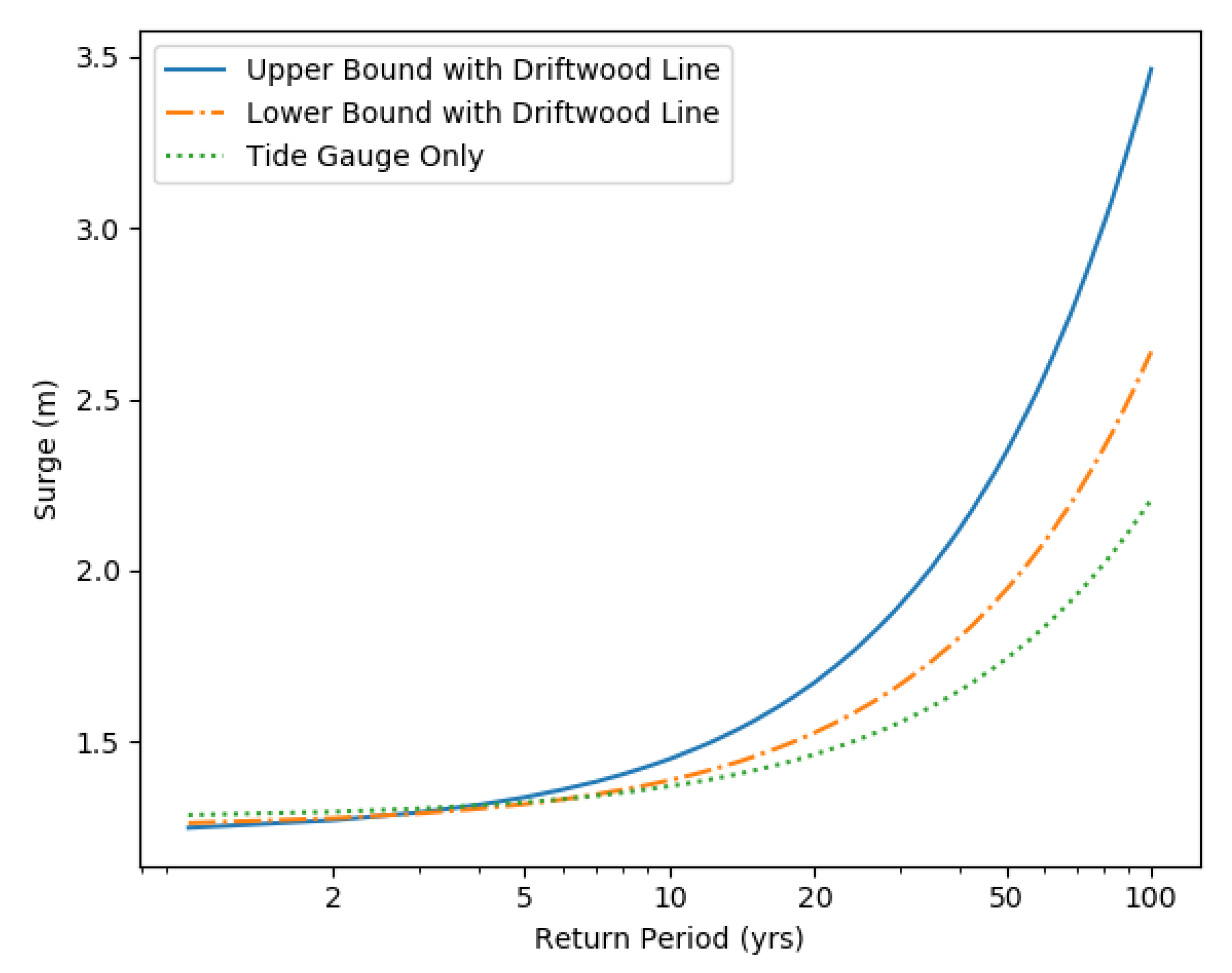
- Inferences based on driftwood surveys and astronomical tide predictions identified two historical storm surge events that exceeded all events captured by the regional tide gauges. One of the events was successfully verified by a hindcast using the numerical model.
- Inclusion of the two historical events in an extreme value analysis significantly altered the best fit probability distribution of storm surges in the region, with implications for risk assessment and coastal engineering design.
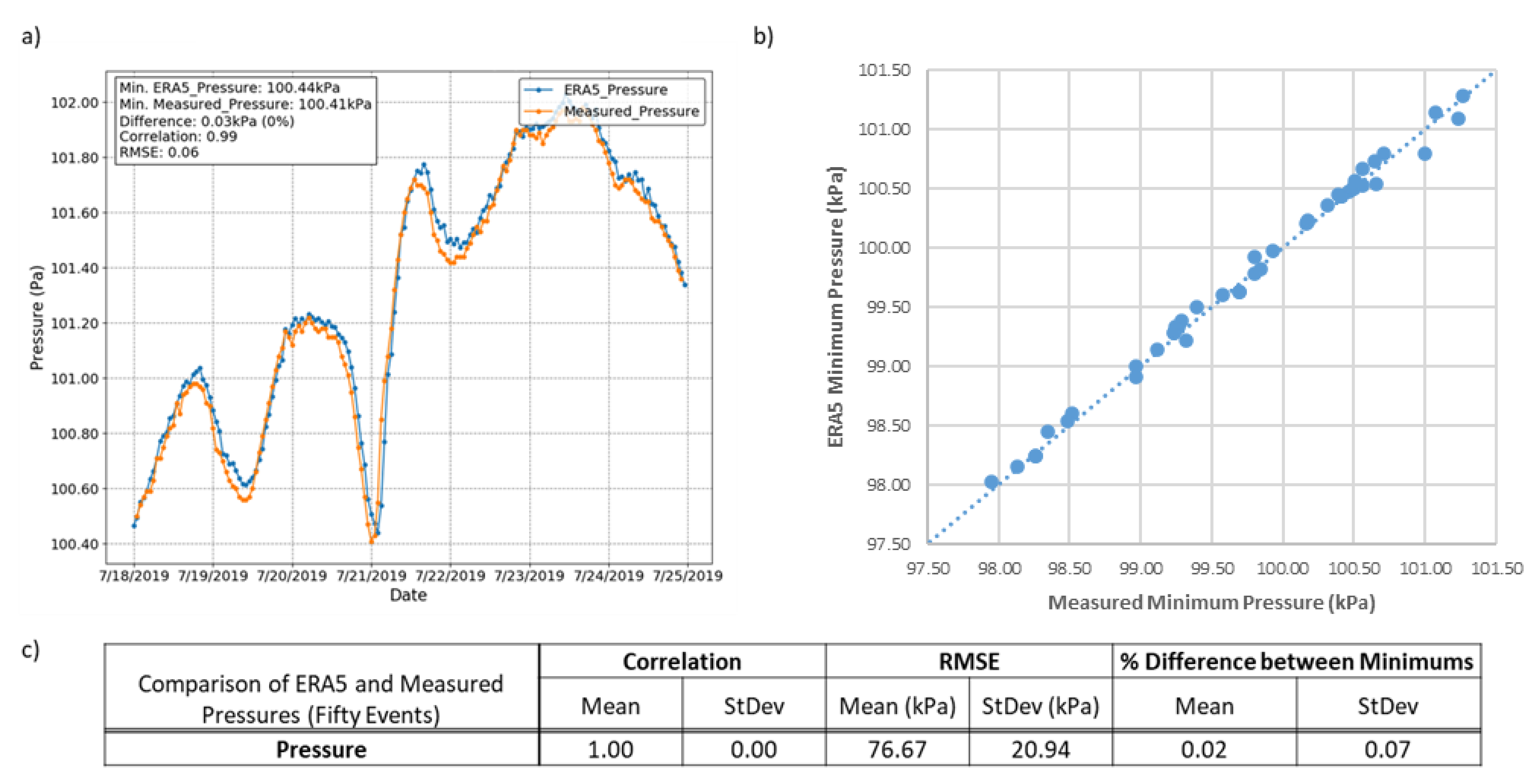
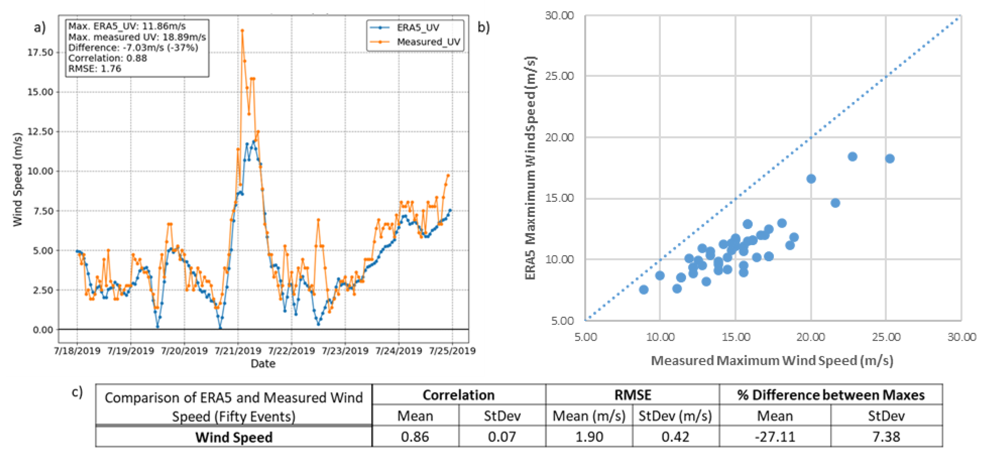
- The ERA5 reanalysis was shown to be an adequate source of surface pressures and wind speeds, except for a systematic underprediction of peak wind speeds at the Tuktoyaktuk weather station. Acceptable numerical modelling results were achieved through calibration of the wind drag coefficient; large wind drag coefficients were prescribed to compensate for the generally low peak wind speeds reported in ERA5.
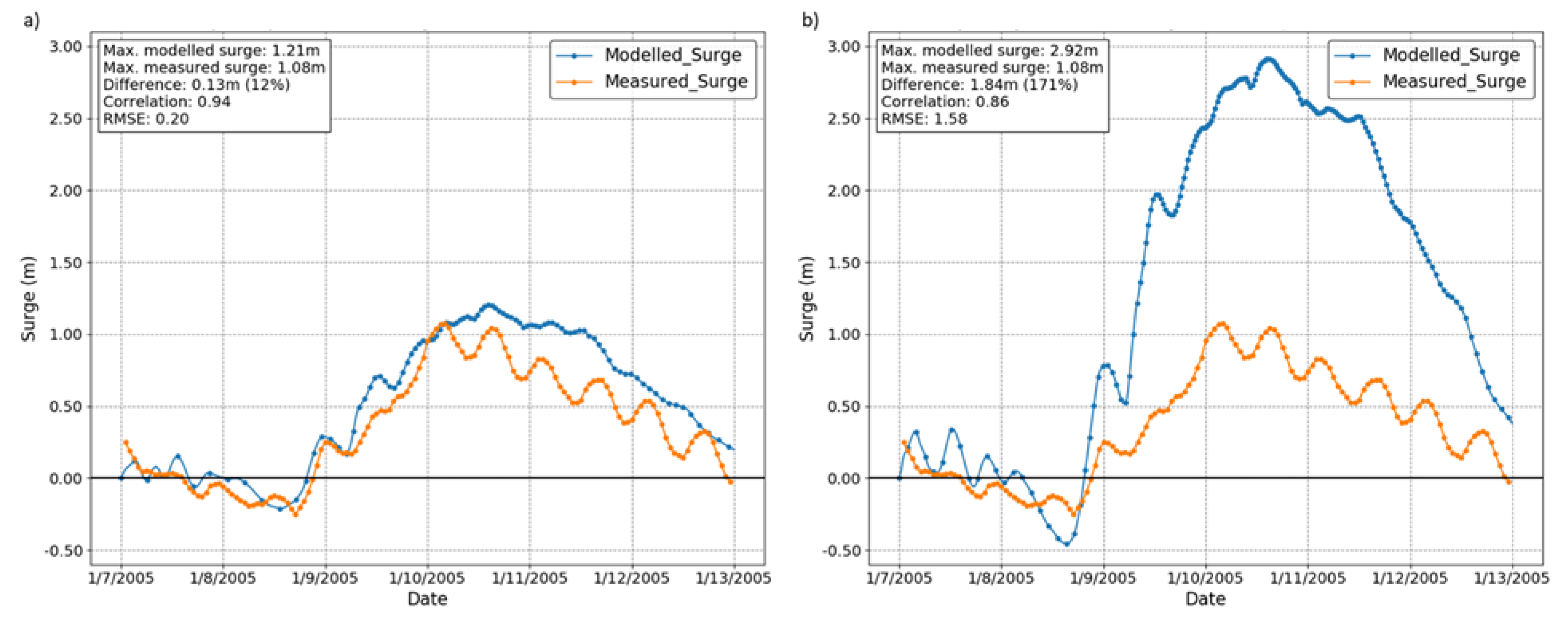
- Sea ice has a significant damping impact on storm surges along the Beaufort Sea coast and should be considered in storm surge analyses for the region. Under open-water scenarios representative of future Arctic conditions, storm surges were found to be as much as three times higher than under present-day ice conditions.
Author Contributions
Funding
Institutional Review Board Statement
Informed Consent Statement
Acknowledgments
Conflicts of Interest
Appendix A

| Rank | Datetime | Measured Residual (m) |
|---|---|---|
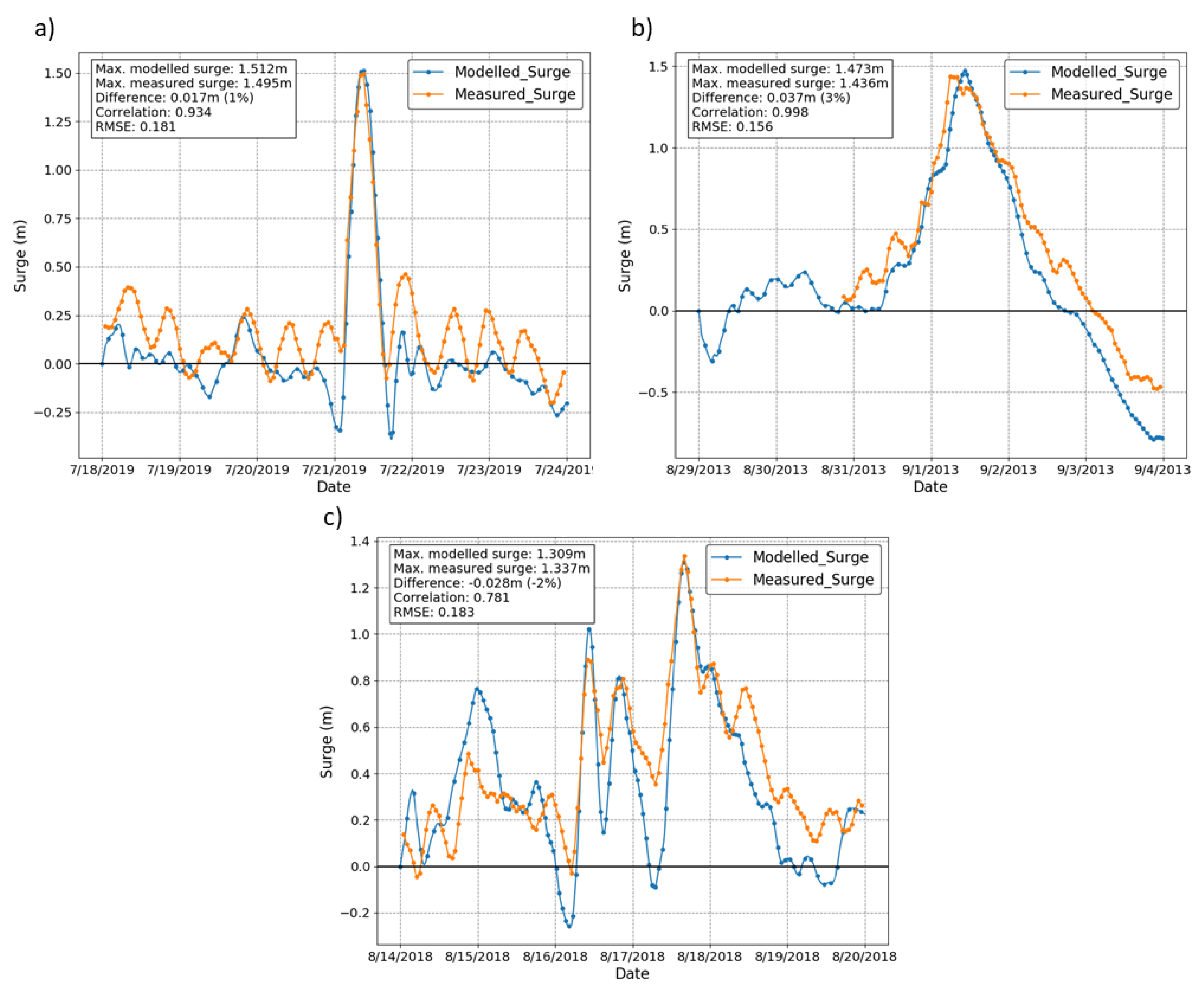
| 1 | 21 July 2019 | 1.49 |
| 2 | 1 September 2013 | 1.44 |
| 3 | 4 November 2017 | 1.42 |
| 4 | 5 August 2019 | 1.40 |
| 5 | 17 August 2018 | 1.34 |
| 6 | 12 September 2003 | 1.27 |
| 7 | 1 September 2018 | 1.25 |
| 8 | 3 September 2018 | 1.25 |
| 9 | 30 October 2013 | 1.23 |
| 10 | 2 August 2004 | 1.17 |
| 11 | 12 November 2013 | 1.17 |
| 12 | 15 November 2013 | 1.17 |
| 13 | 27 August 2015 | 1.12 |
| 14 | 3 September 2016 | 1.12 |
| 15 | 24 August 1991 | 1.11 |
| 16 | 30 July 2008 | 1.11 |
| 17 | 14 August 2004 | 1.08 |
| 18 | 10 January 2005 | 1.08 |
| 19 | 12 August 2019 | 1.07 |
| 20 | 15 August 2019 | 1.07 |
| 21 | 19 November 2010 | 1.05 |
| 22 | 8 September 2016 | 1.04 |
| 23 | 21 August 1982 | 1.03 |
| 24 | 16 September 2003 | 1.02 |
| 25 | 8 October 2008 | 1.00 |
| 26 | 30 August 1980 | 1.00 |
| 27 | 25 July 2017 | 0.99 |
| 28 | 8 October 2019 | 0.99 |
| 29 | 5 July 2018 | 0.99 |
| 30 | 29 October 2003 | 0.98 |
| 31 | 24 August 2019 | 0.97 |
| 32 | 17 August 2019 | 0.96 |
| 33 | 16 September 1980 | 0.96 |
| 34 | 5 October 2019 | 0.95 |
| 35 | 5 October 2003 | 0.94 |
| 36 | 13 October 2019 | 0.90 |
| 37 | 9 August 1991 | 0.90 |
| 38 | 6 August 1991 | 0.90 |
| 39 | 2 November 2019 | 0.90 |
| 40 | 1 October 2015 | 0.90 |
| 41 | 31 October 2019 | 0.88 |
| 42 | 4 September 2009 | 0.88 |
| 43 | 7 September 2009 | 0.88 |
| 44 | 19 September 2016 | 0.87 |
| 45 | 24 September 2016 | 0.86 |
| 46 | 2 January 2010 | 0.83 |
| 47 | 31 July 2018 | 0.82 |
| 48 | 3 December 2003 | 0.82 |
| 49 | 3 July 2006 | 0.82 |
| 50 | 27 September 2003 | 0.81 |
References
- Casas-Prat, M.; Wang, X.; Swart, N. CMIP5-based global wave climate projections including the entire Arctic Ocean. Ocean Model. 2018, 123, 66–85. [Google Scholar] [CrossRef]
- Lemmen, D.S.; Warren, F.J.; James, T.S.; Clarke, C.S.L.M. Canada’s Marine Coasts in a Changing Climate; Natural Resources Canada: Ottawa, ON, Canada, 2016.
- Manson, G.K.; Solomon, S.M. Past and future forcing of Beaufort Sea coastal change. Atmosphere-Ocean 2007, 45, 107–122. [Google Scholar] [CrossRef]
- Bush, E.; Lemmen, D.S. (Eds.) Canada’s Changing Climate Report; Government of Canada: Ottawa, ON, Canada, 2019.
- James, T.S.; A Henton, J.; Leonard, L.J.; Darlington, A.; Forbes, D.L.; Craymer, M. Tabulated values of relative sea-level projections in Canada and the adjacent mainland United States. Geol. Surv. Can. 2015, 7942. [Google Scholar] [CrossRef]
- Ford, J.D.; Couture, N.; Bell, T.; Clark, D.G. Climate change and Canada’s north coast: Research trends, progress, and future directions. Environ. Rev. 2018, 26, 82–92. [Google Scholar] [CrossRef] [Green Version]
- Hoque, A.; Perrie, W.; Solomon, S.M. Evaluation of two spectral wave models for wave hindcasting in the Mackenzie Delta. Appl. Ocean Res. 2017, 62, 169–180. [Google Scholar] [CrossRef] [Green Version]
- Burns, B.M. The Climate of the Mackenzie Valley—Beaufort Sea; Environment Canada, Atmospheric Environment: Toronto, ON, Canada, 1973.
- Henry, R.F. Storm Surges in the Southern Beaufort Sea; Beaufort Sea Project, Department of the Environment: Victoria, BC, Canada, 1974.
- Henry, R.F. Storm Surges; Beaufort Sea Project, Department of the Environment: Victoria, BC, Canada, 1975.
- Henry, R.F.; Heaps, N.S. Storm Surges in the Southern Beaufort Sea. J. Fish. Res. Board Can. 1976, 33, 2362–2376. [Google Scholar] [CrossRef]
- Kowalik, Z. Storm surges in the Beaufort and Chukchi Seas. J. Geophys. Res. Space Phys. 1984, 89, 10570–10578. [Google Scholar] [CrossRef] [Green Version]
- Hersbach, H.; Bell, B.; Berrisford, P.; Hirahara, S.; Horányi, A.; Muñoz-Sabater, J.; Nicolas, J.; Peubey, C.; Radu, R.; Schepers, D.; et al. The ERA5 global reanalysis. Q. J. R. Meteorol. Soc. 2020, 146, 1999–2049. [Google Scholar] [CrossRef]
- Berrisford, P.; Kållberg, P.; Kobayashi, S.; Dee, D.; Uppala, S.; Simmons, A.J.; Poli, P.; Sato, H. Atmospheric conservation properties in ERA-Interim. Q. J. R. Meteorol. Soc. 2011, 137, 1381–1399. [Google Scholar] [CrossRef]
- Dullaart, J.C.M.; Muis, S.; Bloemendaal, N.; Aerts, J.C.J.H. Advancing global storm surge modelling using the new ERA5 climate reanalysis. Clim. Dyn. 2020, 54, 1007–1021. [Google Scholar] [CrossRef] [Green Version]
- Graham, R.M.; Hudson, S.R.; Maturilli, M. Improved Performance of ERA5 in Arctic Gateway Relative to Four Global Atmospheric Reanalyses. Geophys. Res. Lett. 2019, 46, 6138–6147. [Google Scholar] [CrossRef] [Green Version]
- Ramon, J.; Lledó, L.; Torralba, V.; Soret, A.; Doblas-Reyes, F.J. What global reanalysis best represents near-surface winds? Q. J. R. Meteorol. Soc. 2019, 145, 3236–3251. [Google Scholar] [CrossRef] [Green Version]
- Reimnitz, E.; Maurer, D.K. Effects of Storm Surges on the Beaufort Sea Coast, Northern Alaska. Arctic 1979, 32, 329–344. [Google Scholar] [CrossRef] [Green Version]
- Harper, J.R.; Henry, R.F.; Stewart, G.G. Maximum Storm Surge Elevations in the Tuktoyaktuk Region of the Canadian Beaufort Sea. Arctic 1988, 41, 48–52. [Google Scholar] [CrossRef]
- Murty, T.S.; Polavarapu, R.J. Influence of an ice layer on the propagation of long waves. Mar. Geodesy 1979, 2, 99–125. [Google Scholar] [CrossRef]
- Danard, M.B.; Rasmussen, M.C.; Murty, T.S.; Henry, R.F.; Kowalik, Z.; Venkatesh, S. Inclusion of ice cover in a storm surge model for the Beaufort Sea. Nat. Hazards 1989, 2, 153–171. [Google Scholar] [CrossRef]
- Joyce, B.R.; Pringle, W.J.; Wirasaet, D.; Westerink, J.J.; Van Der Westhuysen, A.J.; Grumbine, R.; Feyen, J. High resolution modeling of western Alaskan tides and storm surge under varying sea ice conditions. Ocean Model. 2019, 141, 101421. [Google Scholar] [CrossRef]
- Chapman, R.; Kim, S.-C.; Mark, D. Storm-Induced Water Level Prediction Study for the Western Coast of Alaska. US Army Corps of Engineers. October 2009. Available online: http://www.ariesnonprofit.com/SmithCorpsAKstormSurgeReport.pdf (accessed on 19 August 2020).
- Hervouet, J. Hydrodynamics of Free Surface Flows, 1st ed.; John Wiley & Sons, Ltd.: Hoboken, NJ, USA, 2007. [Google Scholar]
- Fetterer, F.; Knowles, K.; Savoie, M.; Windnagel, A.K. Sea Ice Index; National Snow and Ice Data Center: Boulder, CO, USA, 2017. [Google Scholar] [CrossRef]
- Google. Canada. Available online: https://www.google.com/maps/@71.0146308,-130.9053989,5.83z (accessed on 7 March 2021).
- Foreman, M.G.G.; Cherniawsky, J.Y.; Ballantyne, V.A. Versatile harmonic tidal analysis: Improvements and applications. J. Atmos. Ocean. Technol. 2009, 26, 806–817. [Google Scholar] [CrossRef]
- Serafin, K.A.; Ruggiero, P.; Stockdon, H.F. The relative contribution of waves, tides, and non-tidal residuals to extreme total water levels on US West Coast sandy beaches. Geophys. Res. Lett. 2017, 44, 1839–1847. [Google Scholar] [CrossRef]
- Casas-Prat, M.; Wang, X.L. Projections of Extreme Ocean Waves in the Arctic and Potential Implications for Coastal Inundation and Erosion. J. Geophys. Res. Oceans 2020, 125, 015745. [Google Scholar] [CrossRef]
- Ferreira, J.A.; Soares, C.G. An Application of the Peaks Over Threshold Method to Predict Extremes of Significant Wave Height. J. Offshore Mech. Arct. Eng. 1998, 120, 165–176. [Google Scholar] [CrossRef]
- Brodtkorb, P.A.; Johannesson, P.; Lindgren, G.; Rychlik, I.; Ryden, J.; Sjo, E. WAFO—A Matlab Toolbox for Analysis of Random Waves and Loads. In Proceedings of the International Offshore and Polar Engineering Conference, Seattle, WA, USA, 27 May–2 June 2000; International Society of Offshore and Polar Engineers: Seattle, WA, USA, 2000; p. 8. [Google Scholar]
- Davison, A.C.; Smith, R.L. Models for Exceedances over High Thresholds. J. R. Stat. Soc. Ser. B Stat. Methodol. 1990, 52, 393–425. [Google Scholar] [CrossRef]
- Department of Public Works. Investigation of Storm, September 13–16, 1970—Mackenzie Delta Region, Beaufort Sea; Unpublished Technical Report by Public Works of Canada; Department of Public Works: Los Angeles, CA, USA, 1971. [Google Scholar]
- Weatherall, P.; Marks, K.M.; Jakobsson, M.; Schmitt, T.; Tani, S.; Arndt, J.E.; Rovere, M.; Chayes, D.N.; Ferrini, V.L.; Wigley, R. A new digital bathymetric model of the world’s oceans. Earth Space Sci. 2015, 2, 331–345. [Google Scholar] [CrossRef]
- Barton, A.J. Blue Kenue Enhancements from 2014 to 2019. In Proceedings of the XXVIth Telemac & Mascaret User Conference, Toulouse, France, 15–17 October 2019. [Google Scholar]
- International Hydrographic Organization. Gridded Bathymetry Data (General Bathymetric Chart of the Oceans), GEBCO. 2019. Available online: https://www.gebco.net/data_and_products/gridded_bathymetry_data/ (accessed on 24 August 2020).
- Topf, J. Osmcode/Osmcoastline. GitHub. 2019. Available online: https://github.com/osmcode/osmcoastline (accessed on 20 December 2020).
- World Meteorological Organization. Guide to Storm Surge Forecasting; World Meteorological Organization: Geneva, Switzerland, 2011. [Google Scholar]
- Tolman, H.L. Treatment of unresolved islands and ice in wind wave models q. Ocean Model. 2003, 5, 13. [Google Scholar] [CrossRef]
- Birnbaum, G.; Lüpkes, C. A new parameterization of surface drag in the marginal sea ice zone. Tellus A Dyn. Meteorol. Oceanogr. 2002, 54, 107–123. [Google Scholar] [CrossRef]
- Lüpkes, C.; Gryanik, V.M.; Hartmann, J.; Andreas, E.L. A parametrization, based on sea ice morphology, of the neutral atmospheric drag coefficients for weather prediction and climate models. J. Geophys. Res. Space Phys. 2012, 117. [Google Scholar] [CrossRef] [Green Version]
- CIS. Canadian Ice Service Digital Archive—Regional Chart: History, Accuracy, and Cavetas. CISDA. September 2006. Available online: https://ice-glaces.ec.gc.ca/IA_DOC/cisads_no_001_e.pdf (accessed on 7 March 2021).
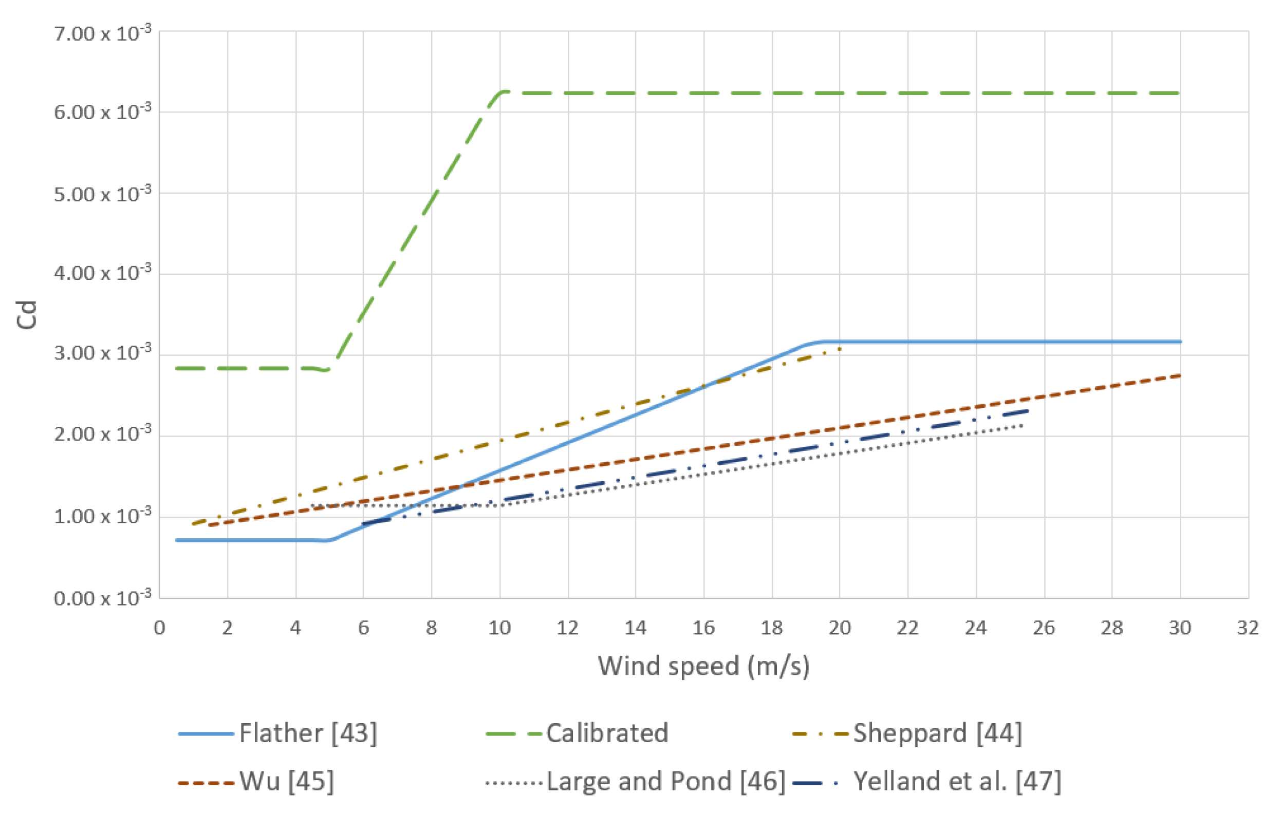
- Flather, R.A. Results from a Storm Surge Prediction Model of the North-West European Continental Shelf for April, November and December 1973; Institute of Oceanographic Sciences: Wormley, UK, 1976. [Google Scholar]
- Sheppard, P.A. Transfer across the earth’s surface and through the air above. Q. J. R. Meteorol. Soc. 1958, 84, 205–224. [Google Scholar] [CrossRef]
- Wu, J. Wind-Stress coefficients over Sea surface near Neutral Conditions—A Revisit. J. Phys. Oceanogr. 1980, 10, 727–740. [Google Scholar] [CrossRef] [Green Version]
- Large, W.G.; Pond, S. Open Ocean Momentum Flux Measurements in Moderate to Strong Winds. J. Phys. Oceanogr. 1981, 11, 324–336. [Google Scholar] [CrossRef] [Green Version]
- Yelland, M.J.; Moat, B.I.; Taylor, P.K.; Pascal, R.W.; Hutchings, J.; Cornell, V.C. Wind Stress Measurements from the Open Ocean Corrected for Airflow Distortion by the Ship. J. Phys. Oceanogr. 1998, 28, 1511–1526. [Google Scholar] [CrossRef]
- Barnhart, K.R.; Miller, C.R.; Overeem, I.; Kay, J.E. Mapping the future expansion of Arctic open water. Nat. Clim. Chang. 2016, 6, 280–285. [Google Scholar] [CrossRef]
- Muis, S.; Apecechea, M.I.; Dullaart, J.; Rego, J.D.L.; Madsen, K.S.; Su, J.; Yan, K.; Verlaan, M. A High-Resolution Global Dataset of Extreme Sea Levels, Tides, and Storm Surges, Including Future Projections. Front. Mar. Sci. 2020, 7, 263. [Google Scholar] [CrossRef]
- Bryant, K.M.; Akbar, M. An Exploration of Wind Stress Calculation Techniques in Hurricane Storm Surge Modeling. J. Mar. Sci. Eng. 2016, 4, 58. [Google Scholar] [CrossRef]
- Forbes, D.L.; Parkes, G.S.; Manson, G.K.; Ketch, L.A. Storms and shoreline retreat in the southern Gulf of St. Lawrence. Mar. Geol. 2004, 210, 169–204. [Google Scholar] [CrossRef]
- Japan Meteorological Agency. JRA-55: Japanese 55-Year Reanalysis, Daily 3-Hourly and 6-Hourly Data; Research Data Archive at the National Center for Atmospheric Research; Computational and Information Systems Laboratory: Boulder, CO, USA, 2013. [Google Scholar]
- Swail, V.R.; Cardone, V.J.; Callahan, B.; Ferguson, M.; Gummer, D.J.; Cox, A.T. The MSC Beaufort Wind and Wave Reanalysis. In Proceedings of the 10th International Workshop on Wave Hindcasting and Forecasting and Coastal Hazard Symp, Oahu, HI, USA, 11–16 November 2007; U.S Army Engineer Research and Development Center: Oahu, HI, USA, 2007; p. 22. [Google Scholar]
- Giusti, M. ERA5 Back Extension 1950–1978 (Preliminary Veresion): Tropical Cyclones Are Too Intense. ECMWF ERA5. November 2020. Available online: https://confluence.ecmwf.int/display/CKB/ERA5+back+extension+1950-1978+%28Preliminary+version%29%3A+tropical+cyclones+are+too+intense (accessed on 20 November 2020).
- Guarino, M.-V.; Sime, L.C.; Schröeder, D.; Malmierca-Vallet, I.; Rosenblum, E.; Ringer, M.; Ridley, J.; Feltham, D.; Bitz, C.; Steig, E.J.; et al. Sea-ice-free Arctic during the Last Interglacial supports fast future loss. Nat. Clim. Chang. 2020, 10, 928–932. [Google Scholar] [CrossRef]


| Rank | Date | Water Level (m CD) |
|---|---|---|
| 1 | 1 September 1944 | 2.95 |
| 1 | 14 September 1970 | 2.95 |
| 3 | 4 October 1963 | 2.23 |
| 4 | 4 September 1962 | 2.15 |
| 5 | 4 November 2017 | 2.02 |
| 6 | 1 September 2013 | 1.96 |
| 7 | 17 August 2018 | 1.95 |
| 8 | 21 July 2019 | 1.94 |
| 9 | 1 September 2018 | 1.89 |
| 10 | 30 July 1963 | 1.85 |
| 11 | 27 August 2015 | 1.82 |
| 12 | 1 September 1962 | 1.78 |
Publisher’s Note: MDPI stays neutral with regard to jurisdictional claims in published maps and institutional affiliations. |
© 2021 by the authors. Licensee MDPI, Basel, Switzerland. This article is an open access article distributed under the terms and conditions of the Creative Commons Attribution (CC BY) license (http://creativecommons.org/licenses/by/4.0/).
Share and Cite
Kim, J.; Murphy, E.; Nistor, I.; Ferguson, S.; Provan, M. Numerical Analysis of Storm Surges on Canada’s Western Arctic Coastline. J. Mar. Sci. Eng. 2021, 9, 326. https://doi.org/10.3390/jmse9030326
Kim J, Murphy E, Nistor I, Ferguson S, Provan M. Numerical Analysis of Storm Surges on Canada’s Western Arctic Coastline. Journal of Marine Science and Engineering. 2021; 9(3):326. https://doi.org/10.3390/jmse9030326
Chicago/Turabian StyleKim, Joseph, Enda Murphy, Ioan Nistor, Sean Ferguson, and Mitchel Provan. 2021. "Numerical Analysis of Storm Surges on Canada’s Western Arctic Coastline" Journal of Marine Science and Engineering 9, no. 3: 326. https://doi.org/10.3390/jmse9030326