Article

A Probabilistic Model of Coastal Bluff-Top Erosion in High Latitudes Due to Thermoabrasion: A Case Study from Baydaratskaya Bay in the Kara Sea

by
Mohammad Akhsanul Islam
1,*,
Raed Lubbad
1 and
Mohammad Saud Afzal
2
1
Department of Civil and Environmental Engineering, Norwegian University of Science and Technology, 7491 Trondheim, Norway
2
Department of Civil Engineering, Indian Institute of Technology Kharagpur, West Bengal 721302, India
*
Author to whom correspondence should be addressed.
J. Mar. Sci. Eng. 2020, 8(3), 169; https://doi.org/10.3390/jmse8030169
Submission received: 30 January 2020 / Revised: 23 February 2020 / Accepted: 28 February 2020 / Published: 3 March 2020
(This article belongs to the Special Issue Coastal Hazards Assessment in Cold Regions)

Abstract

:
Arctic coastal erosion demands more attention as the global climate continues to change. Unlike those along low-latitude and mid-latitude, sediments along Arctic coastlines are often frozen, even during summer. Thermal and mechanical factors must be considered together when analysing Arctic coastal erosion. Two major erosion mechanisms in the Arctic have been identified: thermodenudation and thermoabrasion. Field observations of Arctic coastal erosion are available in Baydaratskaya Bay in the Kara Sea. The objective of this study is to develop a probabilistic model of thermoabrasion to simulate the measured coastal erosion at two sites where observations suggest thermoabrasion is dominant. The model simulates two time periods: (a) the summer of 2013 (2012–2013) and (b) the summer of 2017 (2016–2017). A probabilistic analysis is performed to quantify the uncertainties in the model results. The input parameters are assumed to follow normal and lognormal distributions with a 10% coefficient of variation. Monte Carlo simulation is applied to determine the erosion rates for the two different cases. The simulation results agree reasonably well with the field observations. In addition, a sensitivity analysis is performed, revealing a very high sensitivity of the model to sea-level changes. The model indicates that the relation between sea-level rise and thermoabrasional erosion is exponential.

1. Introduction

Almost one-quarter of the land surface in the Northern Hemisphere is permafrost [1]. The thawing of permafrost releases carbon dioxide and methane on the order of hundreds of gigatons [2]. The American and Canadian coastlines exhibit the highest erosion rates throughout the Arctic region [3]. These annual rates are also among the greatest in the world. In Arctic Alaska, the coastal erosion rates reach as high as 15 m/year [4]. However, if annual erosion within the Arctic is considered only within the open water season window (typically spanning three months), the adjusted erosion rates can be eight times greater than those in the Gulf of Mexico [5]. The alarmingly high rate of present-day erosion is expected to increase due to climate warming [6]. The global climate is confronted with a noticeable shrinkage of the sea-ice cover, and the rate of Arctic land warming is 3.5 times greater than the average 21st century warming rates predicted in global climate models [7].
Accelerated erosion rates have been reported throughout the coastal regions of the Arctic corresponding to the broader spatial extent of open water, the longer open water period and the increased thawing rate of coastal permafrost [8]. Arctic coastal communities are highly affected by rapid coastline retreat, and valuable resources are at risk. Erosion causes large-scale land loss and potential risks to coastal infrastructure, including the oil and gas industry. These conditions are forcing planners to counter the uncertainties and possibilities that arise from rapid erosion [9]. The coastline of the Kara Sea is the longest among all the water bodies within the Arctic Ocean [10] and composes more than one-quarter of the total length of Arctic coastline [11]. Isaev et al. [12] reported erosion rates as high as 29.1 m/year along the coast of the Kara Sea. The mean annual erosion rate along this coast is estimated to be in the range from 0.2 m to 2.0 m per year [13]. Jones et al. [6] reported that the mean annual erosion rate in Alaska along the north-facing coastline between Drew Point and Cape Halkett was 13.6 m/year during 2002 to 2007 and 17.1 m/year during 2007 to 2009.
The mechanisms of Arctic coastal erosion are different from those in warmer regions of low-latitude and mid-latitude [14]. Unlike the coastal erosion occurring on the beaches of low-latitude and mid-latitude coasts, the retreat of coastlines at high latitudes comprises both mechanical and thermal processes. The sediments within bluffs in the Arctic are often permanently frozen. The thawing of permafrost is typically the critical step in the overall sequence of processes leading to coastal erosion. Thermodenudation is the continuous degradation of a frozen coast during the summer by thawing and slump failures. Upon being exposed to warm weather, a portion of a frozen bluff will start to thaw under the impacts of warm air, energy from solar radiation and the melting of snow [15]. When a frozen bluff starts to melt, the mechanical strength of the soil is reduced. At some point, the stability of the slope cannot be maintained, and slope slipping occurs [16]. It was observed that thermodenudation could contribute up to 0.4 m of coastal retreat per year in the Kara Sea, where bluffs are mostly silt and silty clay [17]. On the other hand, thermoabrasion is an episodic yet infrequent phenomenon of Arctic coastal erosion. Bluff failure occurs when a niche destabilises the overhanging portion of the bluff. The mechanical abrasion of the base of the bluffs by the incoming warmer seawater distinguishes thermoabrasion from thermodenudation as water can reach the base of the bluff only during the storms. The three most important environmental parameters responsible for thermoabrasion are the size and position of the ice-wedge polygon and the niche growth rate [18]. Bluff failure can be explained from both geotechnical and hydrodynamic perspectives. From a geotechnical point of view, the authors of [19] proposed that the weight of the overhanging bluff must not exceed the strength of the bluff. Hoque and Pollard [20] proposed a similar model in which bluff collapse can occur along different planes, determined by the mechanical properties of the permafrost and the position of the ice wedge. Kobayashi [21] developed an analytical solution for niche growth during a storm based on the conservation of mass, sediments and salinity. Vidrine [22] developed an integrated solution to the conservation of thermal energy, which was subsequently adopted by Nairn et al. [23] in the software COSMOS 2D. Ravens et al. [24] modelled the erosion occurring at Drew Point, Alaska based on thermoabrasion; they simulated thermoabrasion as a combination of four consequential processes based on simplified physics, and they adopted the [21] model for niche growth. Ravens et al. [24] found that the erosion rate was most sensitive to the elevation of the beach in front of the coastal bluff. Barnhart et al. [4] further improved the model in [24] by using a smaller time-step, relatively more realistic erosion of collapsed bluffs and the application of other niche growth models. Barnhart et al. [4] and Hoque et al. [18] regarded the collapse of the bluff as essentially overturning around the base of the bluff, which was confirmed by field observations. Hoque et al. [18] modelled thermoabrasion as a combination of the tensile strength of frozen soil, the niche depth inside the bluff and the ice-wedge location and depth. However, they did not consider failure along predetermined planes; rather, they postulated that the combination of various environmental parameters determines the failure planes inside the bluff. Isaev et al. [12] estimated the rate of retreat of coastal bluffs based on the relation among the wave energy flux, ground temperature and resistivity of frozen ice-rich material on the premise that the resistivity of frozen materials is significantly higher than that of unfrozen materials. They further observed that wind-driven wave activity during the open water season influences the magnitude of retreat, whereas recent temperature increases contributed relatively little to coastal retreat during the period of 2005 to 2016 along the coastline of the Kara Sea.
In this paper, we develop a numerical model to simulate coastal erosion due to thermoabrasion. The model is based on recent observations and adopts some of the existing modules cited in the literature. Using the Monte Carlo simulation technique, we run the model thousands of times to perform a probabilistic analysis of coastal erosion at two sites of Baydaratskaya Bay in the Kara Sea. The statistical distributions of the inputs for the model are assumed to be normal and lognormal with a 10% coefficient of variation. The parameters of these distributions are estimated from measurements and data available in the literature. The statistical parameters of the distributions of the output (mean and standard deviation) are presented in this paper and compared with available full-scale measurements. We not only validate the model against in situ data, but also investigate the sensitivity of the model to its input parameters. In the following sections, we introduce the study site and the field data. Thereafter, we describe the governing equations of the numerical model, the numerical scheme and the input parameters for the Monte Carlo simulation. Subsequently, we present the model results and discuss the validity of the model against available data and the sensitivity of the model to changes in the input parameters, and we suggest improvements for further work. Finally, we draw the most important conclusions of this study.

2. Field Measurements of Arctic Coastal Erosion in the Kara Sea, Russia

Field measurements of Arctic coastal erosion are available for the coast of Baydaratskaya Bay situated in the Kara Sea (68.853096° N; 66.891730° E), as shown in Figure 1. The field campaign was started in 2012 with support from the Centre for Research-based Innovation (CRI): Sustainable Arctic Marine and Coastal Technology (SAMCoT). The area has been investigated by Lomonosov Moscow State University (MSU) every year since 2012. The measurements are taken at the end of each summer to record the final shoreline position of the year. Soil temperatures are measured throughout the year using thermistor strings (GeoPrecision, Ettlingen, Germany) placed within boreholes drilled in 2012 and 2013. Once summer ends, the shore is covered with snow, and the sea freezes, where sea-ice will also be covered with snow. The sea along the shoreline has a depth of around 10 m which enables large storm surges in the summer (one of the prerequisites for the thermoabrasion process). The region is sporadically populated with very limited infrastructure. The study site is located at a distance of 3.6 km in the northwest (NW) direction from the cofferdam of the Bovanenkobo-Uhta gas pipeline [25].

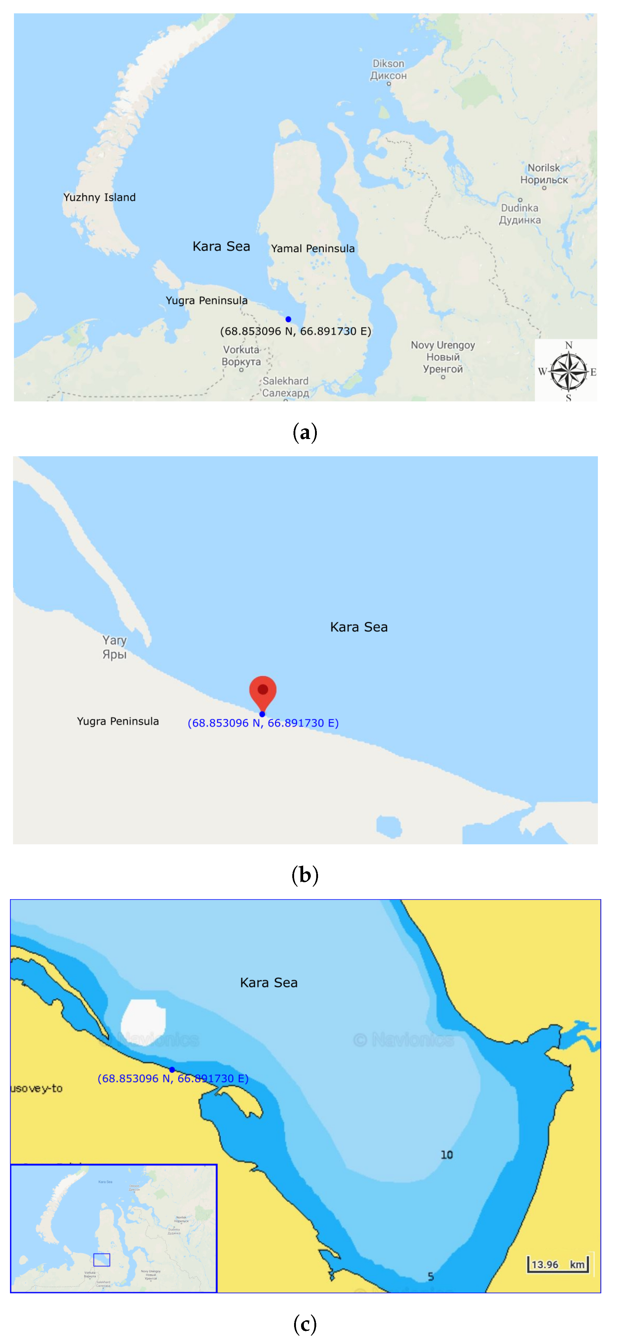
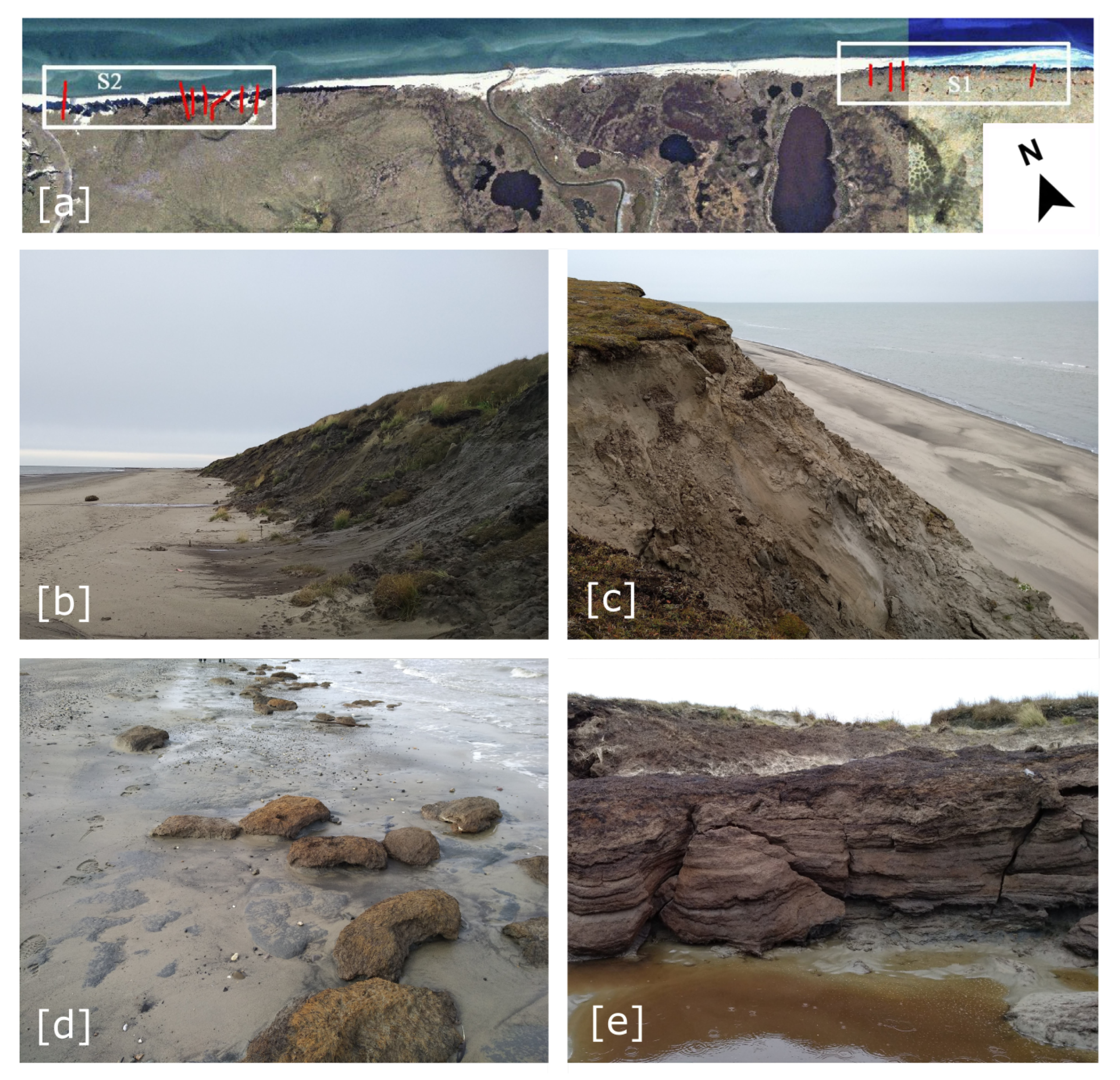
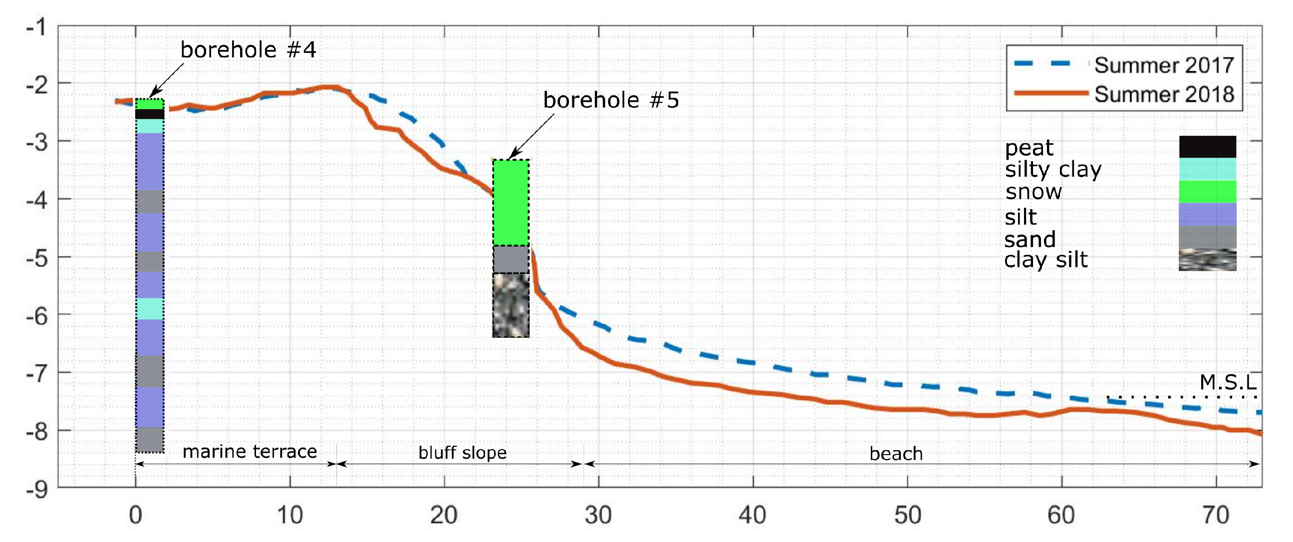
2.1. Geomorphology and Cryology of the Study Area

The Baydaratskaya Bay, situated between the Yugra Peninsula and the Yamal Peninsula, is approximately 350 km long and 250 km wide at its mouth. The study area lies in the northern geocryological zone and features practically continuous permafrost. Three major geomorphological features are distinguishable within the study area: beaches, laida and bluffs. The beaches are sandy and not wider than 50 m. Bluffs with elevations in the range of 4 to 6 m (sandy clay deposits) are termed zone S1, and those with elevations of 12–17 m are termed zone S2 (see Figure 2). The native term “laida” describes a treeless part of the tundra terrain with peat substratum, permafrost close to the surface and covered with low shrubs, mosses and liverworts. The spatial extent of the laida zone is around 500 m along the coast and has been stable in recent years, and is thus excluded from this study. Field measurements have been conducted each year beginning in 2012 with Trimble differential global positioning system (DGPS) equipment in two places: (a) low bluff zones (S1) and (b) high bluff zones (S2) (see Figure 2a). The elevation measurements extend typically a distance of 2 m to 3 m into the open water and the shoreline is noted in the measurements. The exact position of the shoreline at mean sea level is determined via the standard procedure of linear regression of the Lidar data. In total 11 cross-sections were profiled each year. In some of these cross-sections, thermoabrasion was the dominant erosion mechanism. The bluff retreated over a range of 10 to 60 m (average value of 30 m) during the 7 years of observations [25].
Zone S2 is composed of dusty marine sands with a 5 mm thick peat layer and a 10 cm thick ice layer. The land surface in zone S1 is rough and complicated by extensive lake basins in different stages of development. In contrast, the land surface of zone S2 has fewer thermokarst lakes and is covered by a network of ice-wedge polygons [25]. The changes in a typical beach profile in recent years are shown in Figure 3.

2.2. Physical Parameters and Environmental Forcing

The beaches in the study area are 15 m to 50 m wide and are smooth with slightly sloped (0.0015 to 0.0025) sand surfaces lacking vegetation. The bases of the bluffs on the beaches are 1.8 m to 2.3 m above mean sea level. The tidal range of the study area is 0.7 m [26]. Waves reach the base of the bluffs when the storm surges levels are in the range of 1.5 to 2 m. The entire research area is covered by moss and moss-lichen tundra in combination with other types of Arctic tundra [25].
The bay is typically ice-free until the end of September due to thermohaline stratification from warmer and saltier water coming through the Kara Strait [26]. The bay has a salinity range of 20–25 ppt [27]. The tidal currents do not exceed 0.3 m/s [26]. The bay has a depth of less than 10 m near the shore. The currents near the area of interest lie in the range of 0.18 to 0.25 m/s with marginally higher velocities during flooding events [28]. Storm surges in the region can reach 2 m [29], and the root-mean-square wave height (H R M S ) is found to range from 1.3 m to 1.8 m with a peak period of approximately 6 s. The historical rate of recession of the site varies from 0.5 to 1.5 m/year.

3. Conceptual Model of Thermoabrasion

A typical coast with simplified features is considered for the development of the conceptual model (shown in Figure 4). The coast consists of a high, frozen bluff with a narrow beach in front of it. In the calm conditions, the wave run-up does not touch the base of the bluffs. Therefore, only thermodenudation of the bluff is possible: thermoabrasion is possible only when there is water at the base of the bluff. As the base of the bluff is one to few metres above the mean sea level, only during the storm when the surge is significant (1.5–2 m) water reaches the base of the bluffs. Thus, thermoabrasion is episodic and only occurs at the extreme events.
In calm conditions, waves are assumed to break on the beach in front of the frozen bluff and wave hydrodynamics triggers the morphological changes of the beach, which are unrelated to thermoabrasion. During the storm, the beach is submerged and waves with higher energy breaks on the beach due to depth limitation before reaching the base of the bluff. The effect of the waves, return current and erodibility of the soil allows a niche growth at the base of the bluff. As long as there is water at the base of the bluffs, the niche grows inwards. At a critical niche depth, the hanging bluff loses its stability and collapses.
The depth and shape of the niche and growth rate of the niche are influenced by the wave during the storm. The information of the wave is estimated from the water depth since the waves are depth limited on the beach in a similar way the waves are depth limited at surf zone. The depth of the water indirectly determines the wave condition at the base of the bluffs, and thus the extent of a niche inside the bluff can be directly related to the storm surge level (empirical and analytical solution of niche growth is discussed in Section 3.2). The fine sediments cannot sustain the wave actions, and therefore they are transported offshore by return currents. Only relatively coarse sand remains on the beach. The beach is above mean sea level, so water cannot reach the base of the bluff except during the storm. Thawed sediments on the lower part of the beach are removed during high tides.

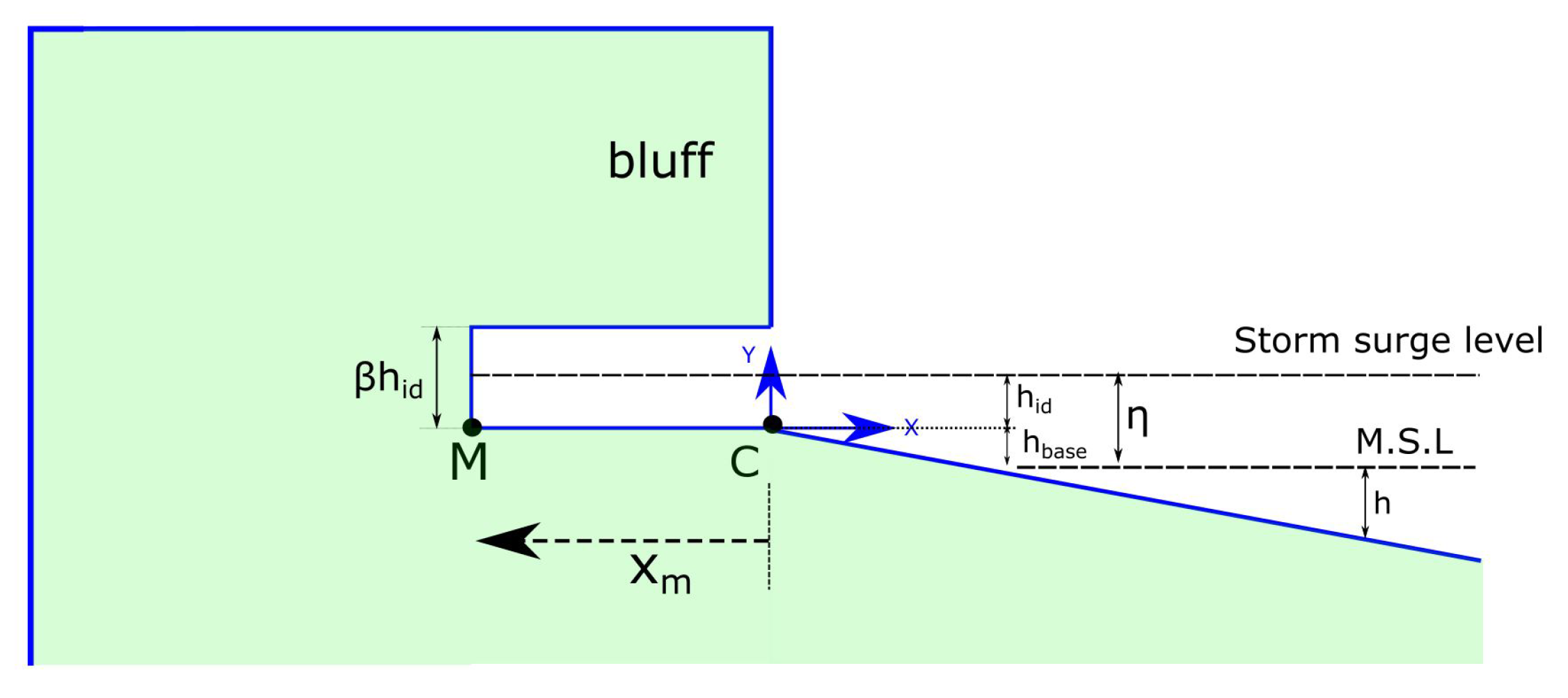
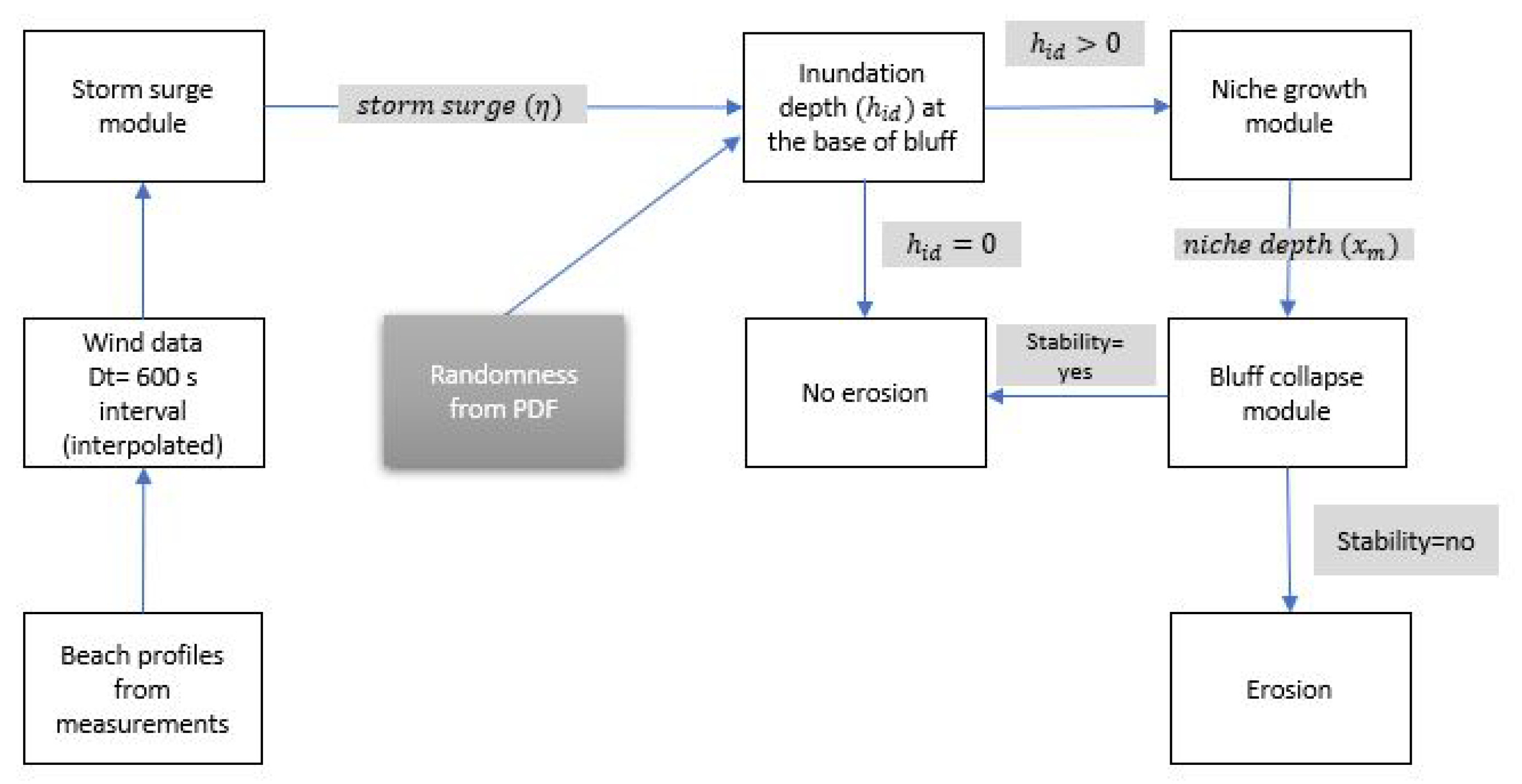
3.1. Storm Surge Module

A one-dimensional simplified storm surge model is adopted to calculate the increase in the water level ( η ) (see Figure 5) from the mean seawater level (M.S.L). The water level rises during a storm due to barometric pressure gradients in the low-pressure storm, the stress coming from wind flows, the Coriolis force induced by earth rotation, and the shape of the bay and the wave set-up. The 1D model described here can not capture the shape of the bay. We also exclude the effect of pressure gradient as the surge level due to the pressure drop is small (less than 10 cm). The generation and propagation of waves during the storm and their effect on the beach profile are omitted from the model since we only focus on the niche at the base of the bluff. The waves are depth-limited on the beach during storms [21], and they break on the narrow beach before reaching the base of the bluff. It is computationally less demanding to estimate only the surge and the inundation depth ( h i d ) at the base of the bluff and assume the wave conditions rather than to simulate the evolution of waves from offshore.
The cross-shore steady-state solution of the equation of motion of Dean and Dalrymple [30] (given in Equation (1)) for a straight and long coast is used as the basis of the storm-surge module:
g · ( h + η ) · d ( h + η ) d x d h d x f · v g = τ s x ρ w
where h = beach water depth, η = increased water level due to storm, g = gravitational acceleration, x = offshore-directed position coordinate, f = Coriolis parameter equal to 2 Ω s i n ϕ ( Ω = angular rate of rotation of the Earth = 7.272 × (10) 5 rad/s), ϕ = latitude of the considered site, v = magnitude of the depth-averaged currents parallel to the shore, d h / d x = slope of the seabed, ρ w = water density (variation due to temperature ignored) and τ s x = shore-normal shear stress on the surface of the water from the wind, calculated as τ s x = ρ w C D U 10 2 , where C D 2 × 10 6 is a drag coefficient and U 10 is the shore normal wind speed at 10 m elevation. Wave-induced set-up and pressure induced surges are not included in this equation.

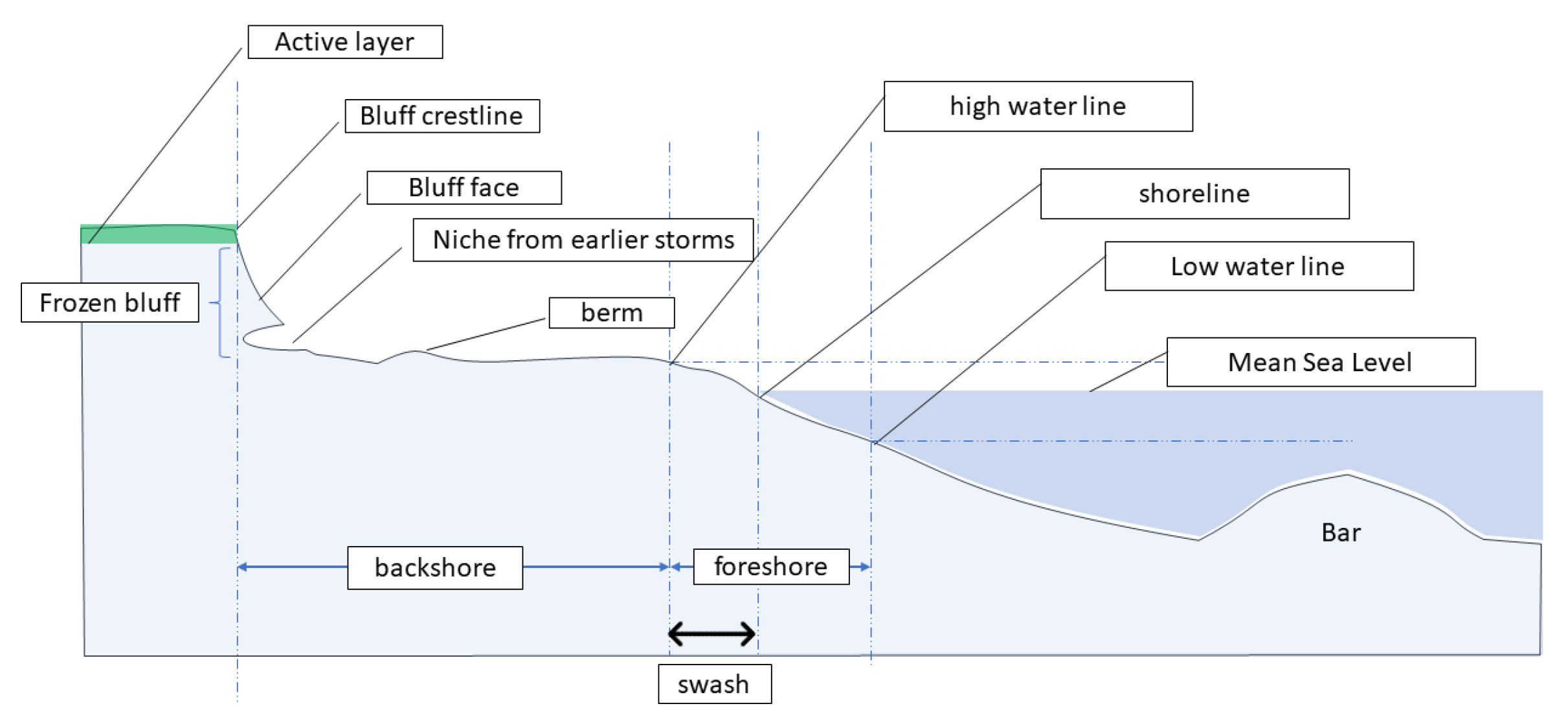
3.2. Niche Growth Module

When the water level reaches the base of the bluff during a storm surge, a niche forms. The niche grows into the bluff; ice present within the bluff starts to melt and some sediments may be extruded. A strong return current generated by the storm washes away these sediments. The analytical solution of niche growth at the base of the bluffs during a storm surge is developed in [21] (given in Equation (2)). Three conservation equations of mass, salinity, and sediments are used to establish the rate of niche growth. To reach the solution, few assumptions are made: (i) waves are depth-limited close to the base of the bluff that means waves break before reaching the base of the bluffs; (ii) the water depth is constant during the growth of the niche; and (iii) the diffusivity constants for the moment, salinity, and sediment concentration are the same as those in the surf zone given by Longuet-Higgins [31] as ϵ = A h ( g h ) 0.5 (where the empirical parameter A = 0.4 and h is the water depth at surf-zone).
The opening of the niche is assumed to be β h i d (see Figure 5); Kobayashi [21] suggests the typical value of β to be 2. In the model of Kobayashi, the wave conditions near the base of the bluff is estimated from the water depth ( h i d ). Although the assumption of constant water depth at the base of the bluff is required to derive Equation (2), our thermoabrasion module is capable of handling variable water depth by treating it as constant only within each time-step of 600 s. This makes Equation (2) to be applicable within the time step and allows the calculation of the niche depth and height relative to the current water depth.
The major input parameters of niche growth modules are given in Table 1.
Kobayashi et al. [21] reached an analytical solution with these above mentioned input parameters, expressed as follows,
x m = 2 ξ m ( ϵ t ) 0.5
where x m = the niche depth (see Figure 5), t = duration of contact of the water at the base of bluff, ξ m = an empirical parameter related to temperature and ϵ is the diffusivity index, which is determined by the empirical formula of Longuet-Higgins [31] as ϵ = A h ( g h ) 0.5 . Kobayashi [21] determines if the suspended sediment concentration before the storm is zero and salinity of the seawater is 30 ppt, the value of ξ m can be approximated to ξ m = 0.0094 T d , where T d is the difference in temperature between the incoming water temperature and ice melting temperature inside niche (0 °C). Equation (2) represents two driving forces of the thermoabrasion. The parameter ξ m represents the thermal component and ϵ represents the inundation depth and mechanical abrasion by the storm surge.

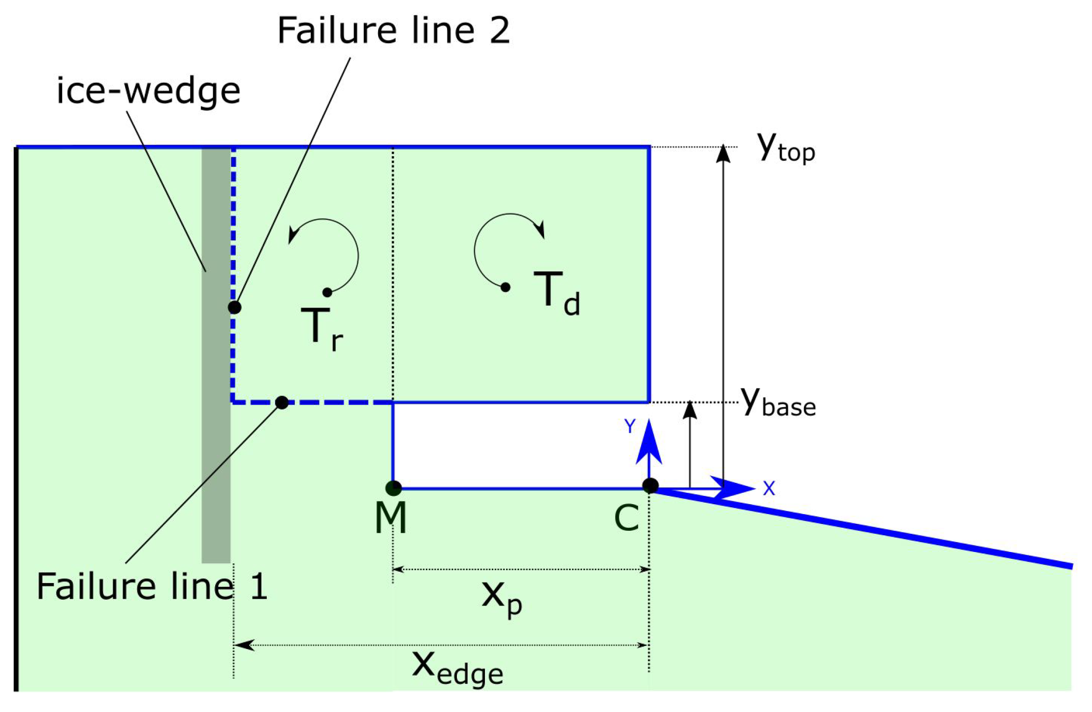
3.3. Bluff Collapse Module

The bluff collapse module is adopted from Barnhart et al. [4] to simulate bluff failure. The model considers the relatively low tensile strength at the ice-wedge boundary. This bluff collapse module is sensitive to the position of the ice-wedge boundary. Therefore, the distribution of ice-wedge polygons at the site is an important parameter for the module. The niche depth at which the bluff collapses is termed the critical niche depth ( x p ). As shown in Figure 6, bluff collapse is determined by the balance of moments around the base of the bluff(point M):
  • the resisting moments, i.e., the self-weight, T r = ρ b g 0 y t o p x e d g e x p ( x p x ) d x d y
  • the moment from the force acting at the vertical failure line, T f = 0 y b a s e τ i ( x e d g e x p ) d y
  • the moment from the force acting at the horizontal failure line, T b = x e d g e x p τ b ( x p x ) d x
  • the moment from the weight of the overhanging bluff, T d = ρ b g y b a s e y t o p 0 x p ( x p x ) d x d y
where x p = niche depth at which the stability is lost, x e d g e = position of the ice-wedge polygon from the base of the bluff, y b a s e = y coordinate of the top of the niche growth melting point, y t o p = y coordinate of the top of the bluff, ρ b = density of the bluff, g = gravitational acceleration, τ b = the tensile strength of the frozen bluff and τ i = tensile strength of ice.
The governing equation for the stability is given in Equation (3):
ρ b g y b a s e y t o p 0 x p ( x p x ) d x d y = ρ b g 0 y t o p x e d g e x p ( x p x ) d x d y + x e d g e x p τ b ( x p x ) d x + 0 y b a s e τ i ( x e d g e x p ) d y
After the failure of the bluff, the collapsed block is disregarded from the model and the bluff is exposed immediately to the water.

3.4. Numerical Scheme

For the numerical parameterization of the governing equations, an explicit Euler scheme is used. The numerical model has a time step of 10 min (600 s) for the three modules. The grid size is 1 m for the storm surge module and bluff collapse module, but a higher spatial resolution (10 cm) is used for the niche growth module since this module is more sensitive. The algorithm for the interaction between the three modules is explained in Figure 7. The major input parameters for the storm surge module other than the global physical parameters are the bathymetry and shore normal wind speed measured at 10 m elevation. The storm surge module calculates the surge level ( η ) for the particular time step using Equation (1). Then, inundation depth ( h i d ) is calculated, and if only the value of h i d is greater than zero (the condition: water reached the base of the bluff is satisfied), it is passed on to the niche growth module as an input parameter. The niche growth module calculates the depth of the niche ( x m ) and passes it to the bluff collapse module. The bluff collapse module checks the stability of the bluff for that time step. If the bluff is stable, no erosion is recorded and the global model moves to the next time step. Table 2 summarises the major input and output parameters of the three modules.
The wind data are obtained from the hindcast model of the NCEP Climate Forecast System Reanalysis (CFSR) provided by the National Oceanic and Atmospheric Administration (NOAA) and downloaded though the Danish Hydraulic Institute (DHI) website.

3.5. Probabilistic Model of Arctic Coastal Erosion

To account for the uncertainties in the input parameters, a probabilistic analysis based on Monte Carlo simulation is carried out. The algorithm of the probabilistic approach is shown in Figure 7. Two assumptions are made: (1) the environmental parameters are independent, i.e., the correlation is set to null, and (2) the coefficient of variation (CoV) is set to be 10%, whereas most of the distributions of the input parameters are considered to follow a normal distribution (details of the distributions and related statistical parameters are shown in Table 3). One-thousand runs are performed for the Monte Carlo simulation using the algorithm depicted in Figure 8.
The parameters of the probabilistic distributions used for the major parameters are given in Table 3.

4. Results and Discussion
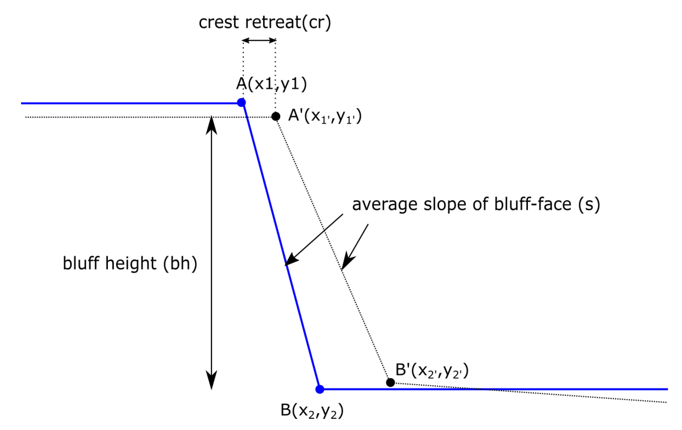
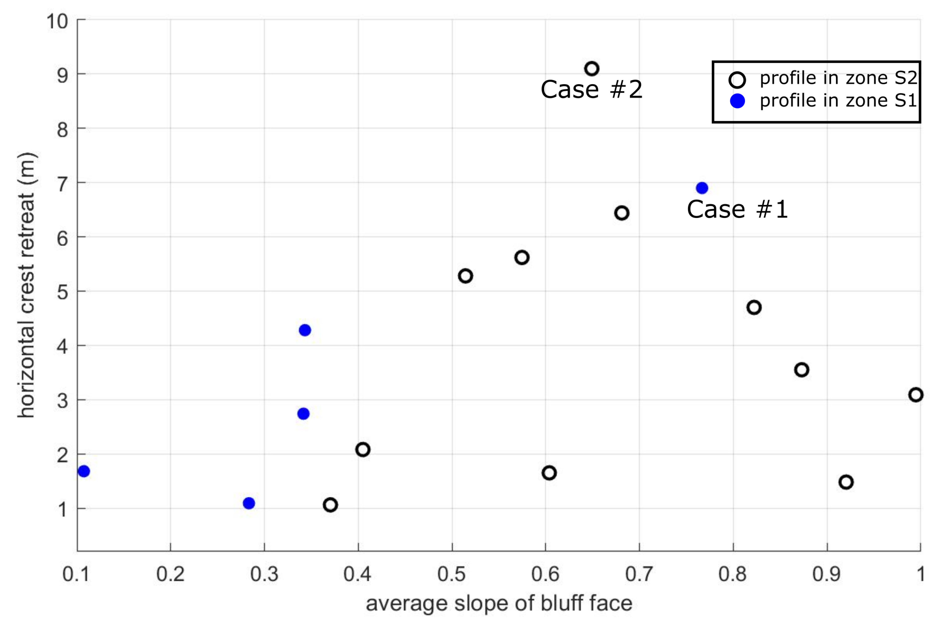
Field measurements are available for eleven profiles at the Baydaratskaya Bay. Isaev et al. [25] reported that both the thermodenudation and thermoabrasion mechanisms are active in the study area. The model can not be applied to all the profiles because some profiles were measured while covered with snow ( mostly in the year 2014 and 2013). The profiles are analysed based on the three geometric criteria:
  • horizontal crest retreat ( c r ),
  • average slope of bluff face (s) and
  • height of the bluff ( b h )
In Figure 9, these parameters are defined as
  • the average slope of the bluff face (s) after the retreat, s = ( y 1 y 2 ) / ( x 1 x 2 )
  • the average slope of the bluff face (s) before the retreat, s = ( y 1 y 2 ) / ( x 1 x 2 )
  • the bluff heights ( b h ) are defined as, b h = y 1 y 2 and b h = y 1 y 2
  • the horizontal crest retreat ( c r ) is defined as, c r = x 1 x 1
Crest retreat ( c r ), bluff height ( b h ) and slope of the bluff-face (s) of the 11 profiles are summarised in Table 4. As the profiles are not continuously measured during the open water season, it is not possible to accurately attribute the annual erosion rate to thermodenudation and thermoabrasion. Field observations suggest thermoabrasion is the dominating erosion mechanism where the slope of the bluff-face is steep (enables bluff collapse) and the crest retreat is high (episodic, infrequent and high erosion). Out of all the profiles, the following 16 cases shown in Figure 10 are retained when we apply the filter: s > 0.1 and c r > 0.1 m. The top right corner of the figure indicates a high annual crest retreat and steep bluff-face slope: two indicators of thermoabrasion.
Two profiles are selected for numerical modelling, namely, Case #1 (zone S1) and Case #2 (zone S2) (shown in Figure 11 and Figure 12, respectively), where observation suggest that thermoabrasion is the dominating erosion mechanism and thus suitable for our current model.
Cases #1 and #2 originate from different time periods and exhibit different geological characteristics (average bluff heights of 5.2 m vs. 14 m, respectively), making the assumption of mutual exclusivity reasonably valid. Case #1 is chosen from the low-lying bluffs with an average height of 5 m. The profile was measured at the ends of the summer seasons of 2012 and 2013. As the sea and the coasts are covered during the rest of the year, bluff erosion can be possible only during the summer. Therefore, for Case #1, the erosion measured along the profile occurred in the summer of 2013. Similarly, for Case #2, the measurements were completed at the ends of the summer seasons of 2016 and 2017, indicating that the erosion measured in Case #2 occurred during the summer of 2017. The niche is more prominent at the location of Case #2 than at that of Case #1 [25]. The wind roses of the two time periods indicate the storm’s directions are almost perpendicular to the coast which satisfies the limitation of the 1D model condition.

4.1. Determination of Crest Retreat in the Two Cases

The three numerical modules mentioned in Section 3.1, Section 3.2 and Section 3.3 are coupled together to simulate crest retreat due to thermoabrasion. Degradation of the collapsed bluff is not explicitly modelled as mentioned earlier is Section 3.3, as the field observations suggest the size of the collapsed blocks on the beach are not significantly large enough to halt the incoming seawater during the storm and to prohibit the development of niche at the base behind it [25]. The probabilistic model calculates erosion due to storm surges for one thousand cases; each iteration is different from the others. The output of the numerical model is composed of one-thousand erosion rates per year, which are normally distributed.

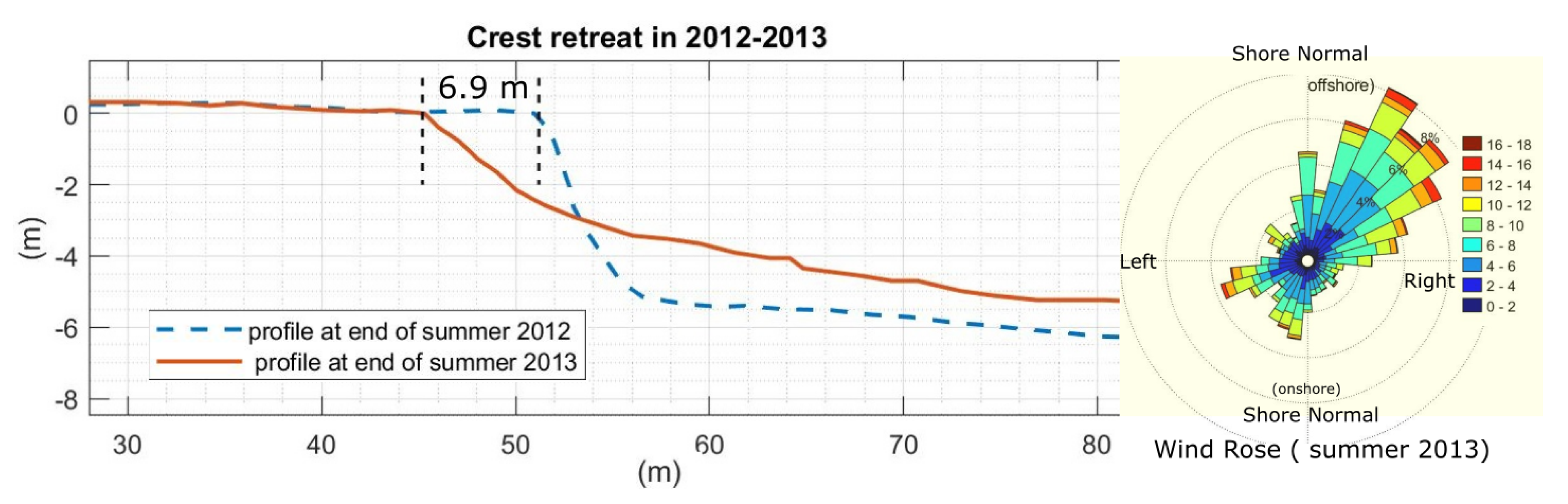
Case #1: Crest Retreat during Summer of 2013

Crest retreat of 6.9 m was measured during the period of 2012–2013 at the mouth of the Sabryavpenzya River, which is termed Case #1, as shown in Figure 11. The model calculates the crest retreat one-thousand times for the Monte Carlo simulation. The value of the crest retreat is considered a random variable following a normal distribution. The mean crest retreat with a 95% confidence limit is calculated to be 6.67 m with a standard deviation of 0.39 m whereas 6.9 m was recorded in the field measurements. Figure 11 shows the measured bed profile for Case #1, whereas subfigure d in Figure 13 shows the cumulative mean erosion during the summer of 2013.

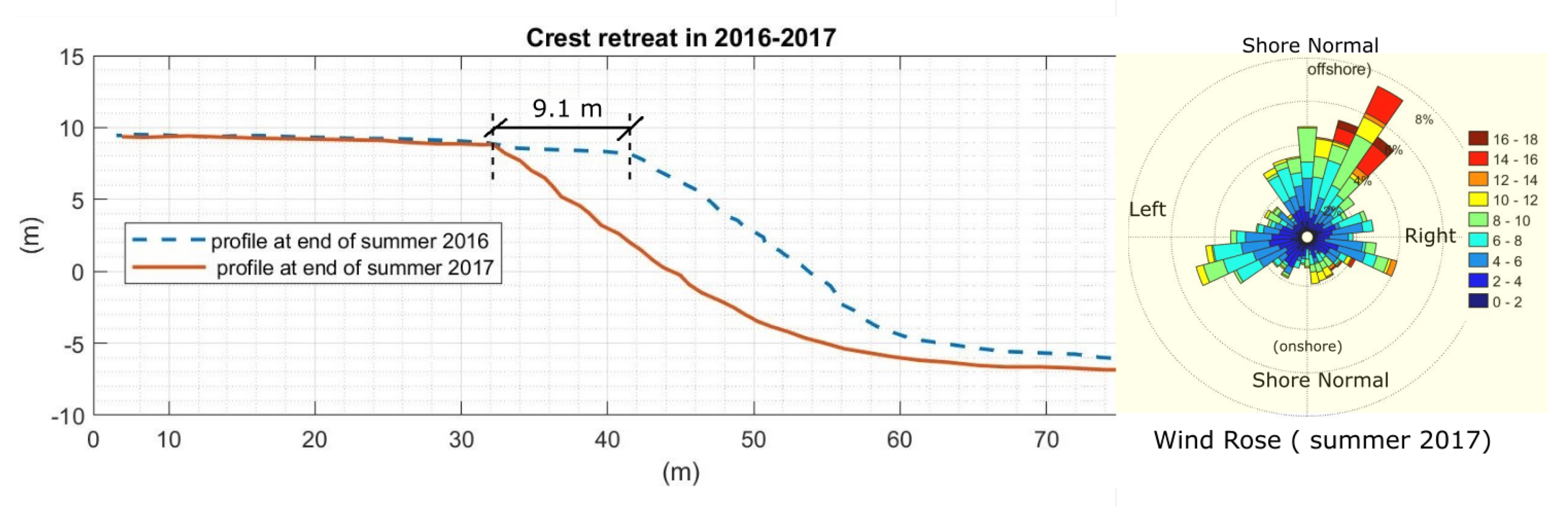
Case #2: Crest Retreat during the Summer of 2017

The crest retreat to the left of the mouth of the Sabryavpenzya River was measured to be 9.1 m during the period of 2016–2017 [12]. This part of the coast has higher frozen bluffs (14 m) than the bluffs in Case #1, and the slope of the bluff face is almost vertical. Similar to Case #1, one-thousand samples of input parameters are generated for the Monte Carlo simulation, and the erosion is calculated as a random variable which follows a normal distribution. A mean erosion of 8.31 m is calculated with a standard deviation of 0.49 m. Figure 14 shows the mean cumulative erosion time series.
The numerical model determined the erosion rates for the two different cases (as detailed in Table 5). The assumption of mutual exclusivity is validated from the erosion patterns of the two cases. Case #1 shows many small storms in 2013 that almost continuously caused erosion throughout the summer season, whereas the profile of Case #2 shows only a few early storms in 2017 that caused abrupt but short-term erosion; few events occurred throughout the rest of the summer season. It is also observed that the numerical model underestimates the erosion by 3.4% for Case #1 and 8.8% for Case #2. The numerical model considers only thermoabrasion, which is a simplification of reality since other erosion mechanisms certainly exist. This may be the reason why the numerical model underestimates the erosion relative to the field measurements. However, the model performance serves as proof of concept, and the behaviour is found to agree with the expected real-world physics.

4.2. Sensitivity Analysis

The numerical model developed in this study considers only thermoabrasional erosion, and thus cannot be applied universally. As this model works in a data-poor environment, a proper understanding of the responses of the numerical model must be achieved. A sensitivity analysis was performed on the probability of bluff failure (shown in Figure 15). It is found that the probability of bluff failure ranges from null to negligible during the first three hours of the storm. Afterwards, the probability of failure exhibits a linear relation with the duration of the storm and niche growth.
The sensitivity analysis results of the other variable environmental conditions are shown in Table 6.
The model is sensitive to the critical niche depth ( x p ); a shorter critical niche depth increases the rate of erosion. The critical niche depth is dependent on the ice-wedge polygon size ( x e d g e ). A sensitivity analysis of the Barnhart [4] model indicates that the relation between x p and x e d g e is linear; a larger polygon size increases the critical niche depth and thus decreases the probability of bluff failure.

5. Conclusions

A theoretical model is developed based on field observations of the physical processes involved in coastal erosion due to thermoabrasion. The governing equations of the theoretical model are based on fundamental physics, e.g., the conservation of mass, energy, salinity and sediments. The governing equations are discretised in time and space. A probabilistic analysis is performed to counter the uncertainties resulting from the data-poor environment. The model is a simplification of real-world physics. It can be only be applied for a short duration since most of the wave hydrodynamics is not included in the model. Out of all the morphological changes due to thermoabrasion, only the crest retreat is simulated. The resulting numerical model can calculate short-term shoreline erosion due to thermoabrasion during storms.
The numerical model is applied to two cases involving different geological features in two different years. The salient outcomes of the numerical model are as follows.
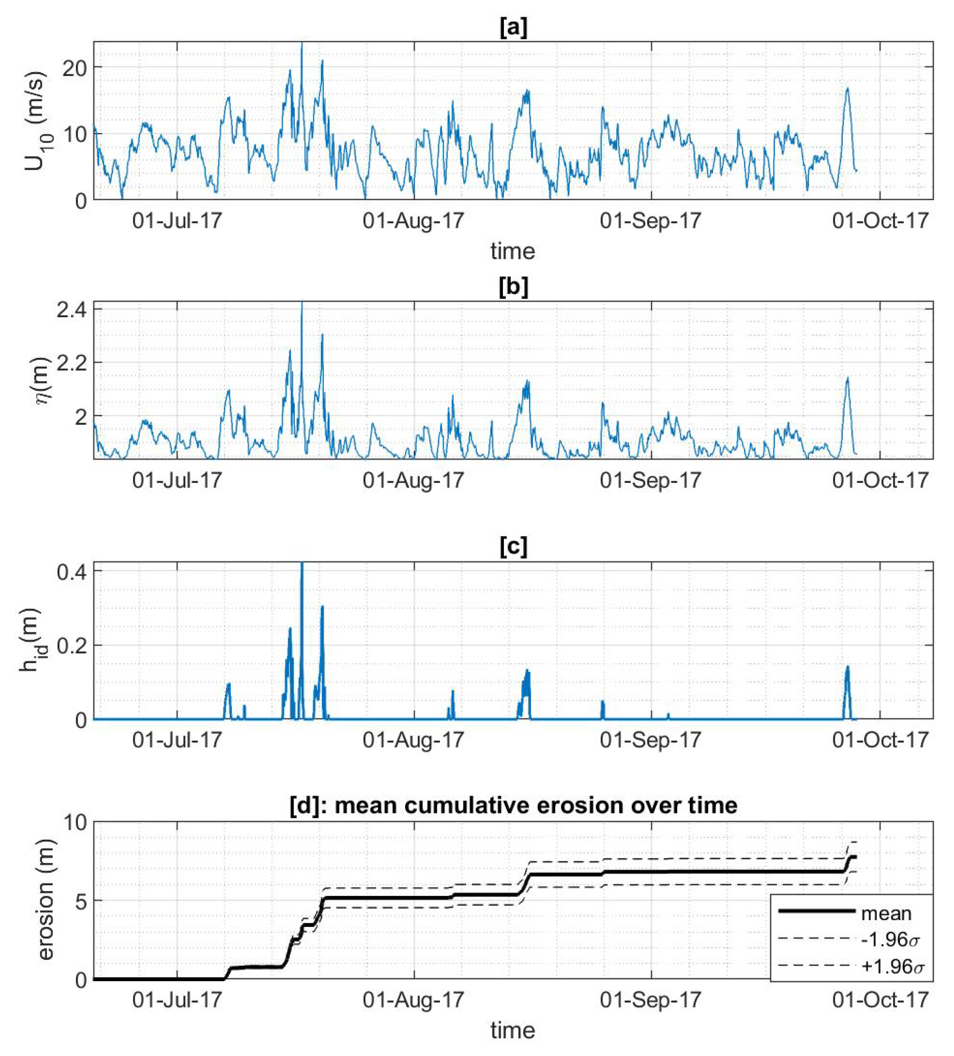
  • Thermoabrasion is episodic and discontinuous, not continuous like other Arctic erosion processes.
  • There is a small time-lag between the inundation depth h i d and niche growth rate. This time lag can be attributed to the initial resistance of the bluff face to the growth of a niche.
  • Coastal erosion is dependent on the intensity of extreme events. Even though Case #1 faced more storms during 2013, the erosion in Case #2 during 2017 is higher than that in Case #1 in 2013 as the intensity and duration of extreme events were significantly higher in 2017.
A sensitivity analysis is carried out to determine the impacts of changes in the environmental parameters. The key findings of the analysis are as follows.
  • The growth of the niche mainly depends on the inundation depth at the base of the bluff, the temperature of incoming waves and the wave height (which is depth-limited).
  • The thermoabrasion process is highly sensitive to changes in sea level; therefore, the coasts where thermoabrasion is the dominant erosion process are at higher risk under sea-level rise.
  • The sediment concentration and salinity of seawater have very little effect on thermoabrasion when compared to the other input parameters.
  • The sensitivity analysis also reveals that the height of the bluff is a secondary factor for thermoabrasion. Field observations also validated this.
The model developed in this study assumes simplified physics, and thus has a very low computational demand at the price of sacrificing information about wave hydrodynamics and morphological changes. This low demand for computational resources allows the model to run one thousand times for the Monte Carlo simulations. A high number of cases is important for a probabilistic model, such as a Monte Carlo simulation. Even though the model is preliminary and simplified, only a 10-min time-step is used, which is a rather dense resolution when compared with similar kinds of models. For example, the authors of [24] used a time-step of 12 h for their model and the comprehensive model in [4] uses time step of 60 min.
The model described herein is a 1D model that considers sediment transport only in the cross-shore direction, similar to many Arctic erosion models. Moreover, we only considered the longshore current; the model does not calculate the longshore sediment transport or nearshore hydrodynamics, such as wave breaking, shoal formation and current-wave interactions. From the field observations, it is clear that similar to the low-latitude and mid-latitude coasts, longshore sediment transport in the Arctic coast is responsible for long-term changes in the shoreline even though the open water season is only three months. The current model considers only the effects of storms, so longshore sediment transport is excluded since the morphological footprint of longshore sediment transport takes a considerable amount of time to be visible. For a long-term prediction of shoreline changes, various additional parameters, including longshore sediment transport, wave evolution, and changes in bathymetry, must be incorporated into the model.
The current model focuses on the two driving forces of thermoabrasional erosion during a storm: (a) the thermal driving force originating from warm sea water and (b) the mechanical driving force of storm surge. Field observations indicate that thermoabrasional erosion is prominent in ice-rich bluffs consist of clay sediments. Clay sediments extruded from the degraded collapsed block are not deposited near swash zones; rather, they are most likely carried off to the deep sea by the strong return currents generated by storm surges. As such, clay sediments do not contribute to beach development. Based on this observation, cross-shore fine sediment transport is excluded from the current model. However, both the cross-shore transport of clay sediments and the longshore transport of sandy sediments are important for long-term predictions of shoreline positions. The global model can be applied to other coasts where thermoabrasion is the dominating erosional mechanisms. The model can be used for other coasts in the Arctic region without modification as no empirical formula is used. Even though in theory the model can be used for long-term prediction of the coastal erosion, we can not suggest it as other environmental parameters which are omitted in the model become important in longer duration model run.
The success of the proposed model, which predicts erosion with probabilistic statistics, serves as a proof of concept. For low-quality metocean information available on the Arctic coasts, the potential to predict shoreline changes and the probability of bluff failure may be valuable for planning and protection endeavours.

Author Contributions

Conceptualisation, M.A.I., R.L. and M.S.A.; formal analysis, M.A.I. and M.S.A.; methodology, M.A.I.; validation, M.A.I., R.L. and M.S.A.; software, M.A.I.; resources, M.A.I., R.L. and M.S.A.; data collection, M.A.I. and R.L.; writing—original draft preparation, M.A.I. and M.S.A.; writing—review and editing, M.A.I., R.L. and M.S.A.; investigation, M.A.I. and M.S.A.; supervision, R.L. and M.S.A.; project administration, R.L. and M.S.A. All authors have read and agreed to the published version of the manuscript.

Funding

This research was funded by the EU H2020-funded Nunataryuk project, where it is filed as part of deliverable 6.4, and by the NCPOR//PACER Outreach Programme (POP) Initiative on “Predictive Tools for Arctic Coastal Hydrodynamics and Sediment Transport”.

Acknowledgments

The report is written as part of the EU H2020-funded Nunataryuk project, where it is filed as part of deliverable 6.4, and by the NCPOR//PACER Outreach Programme (POP) Initiative on “Predictive Tools for Arctic Coastal Hydrodynamics and Sediment Transport”. This research is also supported by Sustainable Arctic Marine and Coastal Technology (SAMCoT), Norwegian University of Science and Technology (NTNU), Lomonosov Moscow State University (MSU) and Sponsored Research and Industrial Consultancy (SRIC), Indian Institute of Technology Kharagpur.

Conflicts of Interest

The authors declare no conflicts of interest.

References

  1. Zhang, T.; Barry, R.G.; Knowles, K.; Heginbottom, J.; Brown, J. Statistics and characteristics of permafrost and ground-ice distribution in the northern hemisphere. Polar Geogr. 1999, 23, 132–154. [Google Scholar] [CrossRef]
  2. Anisimov, O.; Reneva, S. Permafrost and changing climate: The Russian perspective. Ambio 2006, 35, 169–175. [Google Scholar] [CrossRef]
  3. Frederick, J.M.; Thomas, M.A.; Bull, D.L.; Jones, C.A.; Roberts, J.D. The Arctic Coastal Erosion Problem; Technical Report SAND2016-9762; Sandia National Laboratories: Albuquerque, NM, USA, 2016.
  4. Barnhart, K.R.; Anderson, R.S.; Overeem, I.; Wobus, C.; Clow, G.D.; Urban, F.E. Modeling erosion of ice-rich permafrost bluffs along the Alaskan Beaufort Sea coast. J. Geophys. Res. Earth Surf. 2014, 119, 1155–1179. [Google Scholar] [CrossRef]
  5. Reimnitz, E.; Graves, S.M.; Barnes, P.W. Beaufort Sea Coastal Erosion, Sediment Flux, Shoreline Evolution, and the Erosional Shelf Profile; U.S. Geological Survey: Reston, VA, USA, 1988.
  6. Jones, B.M.; Arp, C.D.; Jorgenson, M.T.; Hinkel, K.M.; Schmutz, J.A.; Flint, P.L. Increase in the rate and uniformity of coastline erosion in Arctic Alaska. Geophys. Res. Lett. 2009, 36. [Google Scholar] [CrossRef]
  7. Lawrence, D.M.; Slater, A.G.; Tomas, R.A.; Holland, M.M.; Deser, C. Accelerated Arctic land warming and permafrost degradation during rapid sea ice loss. Geophys. Res. Lett. 2008, 35. [Google Scholar] [CrossRef] [Green Version]
  8. Ravens, T.; Peterson, S.; Panchang, V.; Kaihatu, J. Arctic coastal erosion modeling. In Advances in Coastal Hydraulics; World Scientific: Singapore, 2018; p. 47. [Google Scholar]
  9. Prowse, T.D.; Furgal, C.; Chouinard, R.; Melling, H.; Milburn, D.; Smith, S.L. Implications of climate change for economic development in northern Canada: Energy, resource, and transportation sectors. Ambio 2009, 38, 272–281. [Google Scholar] [CrossRef] [PubMed]
  10. Soluri, E.; Woodson, V. World vector shoreline. Int. Hydrogr. Rev. 1990, 67, 27–35. [Google Scholar]
  11. Lantuit, H.; Overduin, P.P.; Couture, N.; Wetterich, S.; Aré, F.; Atkinson, D.; Brown, J.; Cherkashov, G.; Drozdov, D.; Forbes, D.L.; et al. The Arctic coastal dynamics database: A new classification scheme and statistics on Arctic permafrost coastlines. Estuar. Coasts 2012, 35, 383–400. [Google Scholar] [CrossRef] [Green Version]
  12. Isaev, V.; Koshurnikov, A.; Pogorelov, A.; Amangurov, R.; Podchasov, O.; Sergeev, D.; Buldovich, S.; Aleksyutina, D.; Grishakina, E.; Kioka, A. Cliff retreat of permafrost coast in south-west Baydaratskaya Bay, Kara Sea, during 2005–2016. Permafr. Periglac. Proc. 2019, 30, 35–47. [Google Scholar] [CrossRef]
  13. Baranskaya, A.; Belova, N.; Kokin, O.; Shabanova, N.; Aleksyutina, D.; Ogorodov, S. Coastal dynamics of the Barents and Kara Seas in changing environment. In Proceedings of the 13th International MEDCOAST Congress on Coastal and Marine Sciences, Engineering, Management & Conservation, Mellieha, Malta, 31 October–4 November 2017; Volume 1, pp. 281–292. [Google Scholar]
  14. Afzal, M.S.; Lubbad, R. Development of predictive tool for coastal erosion in Arctic—A review. In Proceedings of the Fourth International Conference in Ocean Engineering (ICOE2018); Murali, K., Sriram, V., Samad, A., Saha, N., Eds.; Springer: Singapore, 2019; pp. 59–69. [Google Scholar]
  15. Guégan, E. Erosion of Permafrost Affected Coasts: Rates, Mechanisms and Modelling; NTNU: Trondheim, Norway, 2015. [Google Scholar]
  16. Pearson, S.; Lubbad, R.; Le, T.; Nairn, R. Thermomechanical erosion modelling of Baydaratskaya Bay, Russia with COSMOS. In Scour and Erosion, Proceedings of the 8th International Conference on Scour and Erosion (Oxford, UK, 12–15 September 2016); CRC Press: Boca Raton, FL, USA, 2016; p. 281. [Google Scholar]
  17. Vasiliev, A.; Kanevskiy, M.; Cherkashov, G.; Vanshtein, B. Coastal dynamics at the Barents and Kara Sea key sites. Geo Mar. Lett. 2005, 25, 110–120. [Google Scholar] [CrossRef] [Green Version]
  18. Hoque, M.A.; Pollard, W.H. Stability of permafrost dominated coastal cliffs in the Arctic. Polar Sci. 2016, 10, 79–88. [Google Scholar] [CrossRef]
  19. Harper, J.R. The Physical Processes Affecting the Stability of Tundra Cliff Coasts. 1978. Available online: digitalcommons.lsu.edu (accessed on 30 January 2020).
  20. Hoque, M.A.; Pollard, W.H. Arctic coastal retreat through block failure. Can. Geotech. J. 2009, 46, 1103–1115. [Google Scholar] [CrossRef]
  21. Kobayashi, N. Formation of thermoerosional niches into frozen bluffs due to storm surges on the Beaufort Sea coast. J. Geophys. Res. Oceans 1985, 90, 11983–11988. [Google Scholar] [CrossRef]
  22. Kobayashi, N.; Vidrine, J.C. Combined Thermal-Mechanical Erosion Processes Model; Center for Applied Coastal Research, University of Delaware: Newark, DE, USA, 1995. [Google Scholar]
  23. Nairn, R.; Solomon, S.; Kobayashi, N.; Virdrine, J. Development and testing of a thermal-mechanical numerical model for predicting Arctic shore erosion processes. In Permafrost, Proceedings of the Seventh International Conference, Yellowknife, NWT, Canada, 23–27 June 1998; Centre d’études nordiques, Université Laval: Laval, QC, Canada, 1998; pp. 789–795. [Google Scholar]
  24. Ravens, T.M.; Jones, B.M.; Zhang, J.; Arp, C.D.; Schmutz, J.A. Process-based coastal erosion modeling for drew point, North Slope, Alaska. J. Waterw. Port Coast. Ocean Eng. 2011, 138, 122–130. [Google Scholar] [CrossRef] [Green Version]
  25. Isaev, V.; Kokin, O.; Pogorelov, A.; Gorshkov, E.; Komarov, O.; Amangurov, R.; Simonsen, V. Field Investigation and Laboratory Analyses Baydaratskaya Bay 2018; Norwegian University of Science and Technology: Trondheim, Norway, 2019. [Google Scholar] [CrossRef]
  26. Harms, I.; Karcher, M. Modeling the seasonal variability of hydrography and circulation in the Kara Sea. J. Geophys. Res. Oceans 1999, 104, 13431–13448. [Google Scholar] [CrossRef]
  27. Stein, R.; Fahl, K.; Fiitterer, D.; Galimov, E.; Stepanets, O. River run-off influence on the water mass formation in the Kara Sea. In Siberian Rer Run-Off in the Kara Sea: Characterisation, Quantification, Variability and Environmental Significance; Elsevier: Amsterdam, The Netherlands, 2003; Volume 6, p. 9. [Google Scholar]
  28. Odisharia, G.; Tsvetsinsky, A.; Mikhailov, N.; Dubikov, G. Specialized information system on environment of Yamal Peninsula and Baydaratskaya Bay. In Proceedings of the 7th International Offshore and Polar Engineering Conference, Honolulu, HI, USA, 25–30 May 1997. [Google Scholar]
  29. Leont’yev, I. Coastal profile modeling along the Russian Arctic coast. Coast. Eng. 2004, 51, 779–794. [Google Scholar] [CrossRef]
  30. Dean, R.G.; Dalrymple, R.A. Coastal Processes with Engineering Applications; Cambridge University Press: Cambridge, UK, 2004. [Google Scholar]
  31. Longuet-Higgins, M.S. Longshore currents generated by obliquely incident sea waves: 1. J. Geophys. Res. 1970, 75, 6778–6789. [Google Scholar] [CrossRef]
Figure 1. The study location is situated along the coast of the Kara Sea and in between the Yugra Peninsula and the Yamal Peninsula. The sea is shallow and funnel-shaped, which makes it susceptible to large storm surges (image source: a and b: Google Earth and c: navionics.com). (a) The study location is along the Kara sea (68.853096° N, 66.891730° E). (b) The beach is located near the 69° N latitude; straight but the orientation is around 45° with horizontalline. (c) Bathymetry of the study area. Near the shore, the depth is 10 m.
Jmse 08 00169 g001
Figure 2. (a) Beach profile lines in zone S1 and zone S2 (thick red lines) from the surface of the bluff to the swash zone of the beach. (b) Bluff in zone S1 and (c) bluff in zone S2. Zone S1 has an uneven bluff surface, a relatively gentle bluff slope and a wide and smooth beach (subfigure (b)), whereas zone S2 comprises a steeper bluff slope and a narrower beach (subfigure (c)). (d) Remnant of an earlier collapsed bluff. Sizes of the collapsed bluff are not big enough to disrupt storm surge and to prohibit the growth of niche at the base of bluffs. However, the active layer with dead vegetation still resists degradation, whereas the rest of the collapsed bluff eroded. (e) Niches in the bluff face. The uneven shape of the niche indicates various levels of storm surges. (image source: (panel (a): [25] and panels (be): authors, summer, 2019)
Jmse 08 00169 g002
Figure 3. Typical cross section at zone S1 depicting the positions of the boreholes. The boreholes are equipped with thermistor strings to measure the temperature every ten minutes at various levels [25].
Jmse 08 00169 g003
Figure 4. Schematic of a typical Arctic coast. A frozen bluff stands at the end of the beach. Storm surges can flood the beach and reach the base of the bluffs where a niche forms.
Jmse 08 00169 g004
Figure 5. Definition of geometrical parameters to estimate the growth of the niche (as per the work in [21]). Point C in the figure is the origin of coordinates (0,0), x m = the depth of niche, h i d = the inundation depth at the base (assumed constant during the time-step of the global model and calculated as h i d = ( η h b a s e ), M is the niche melting front advancing inward, and β h i d is the opening of the niche.
Jmse 08 00169 g005
Figure 6. Stability of an overhanging bluff over a niche. Two failure lines are marked 1 (horizontal) and 2 (vertical). The forces acting along the horizontal failure line creates moment T b at the base of the bluff and forces acting along the vertical failure line creates moment T f . The moment from the overhanging portion ( T d ) is the counterbalancing moment for destabilisation and the rest of the block volume is providing the resisting moment T r . The balance is lost when T d > T r + T b + T w .
Jmse 08 00169 g006
Figure 7. Algorithm of the model with three numerical modules and Monte Carlo simulation.
Jmse 08 00169 g007
Figure 8. Generation of cases for the Monte Carlo simulation.
Jmse 08 00169 g008
Figure 9. Definition of the horizontal crest retreat ( c r ), the average slope of the bluff-face (s) and the height of the bluff ( b h ). The bluff retreated from A’B’ line to now AB line. The crest retreated from point A’( x 1 , y 1 ) to A( x 1 , y 1 ) whereas the base retreated from B’( x 2 , y 2 ) to B( x 1 , y 1 ).
Jmse 08 00169 g009
Figure 10. Thermoabrasion is the dominating erosion mechanism for the cases in the top-right zone (steeper slope and higher erosion rate). Two cases are chosen from zone S1 and zone S2 such that the crest retreat is very high compared to the other profiles and the average slope of the bluff-face is steeper.
Jmse 08 00169 g010
Figure 11. Case #1: The profile is situated in zone S1. Crest retreat of 6.9 m is recorded at the end of the summer of 2013. The wind rose diagram derived from the wind speed data of summer 2013 is shown at the right panel. The diagram is adjusted 49.28° so that shore-normal (offshore) direction is in the top. The wind rose diagram indicates that the dominating wind direction is inclined about 30° towards the shoreline.
Jmse 08 00169 g011
Figure 12. Case #2: The profile is situated in zone S2. Crest retreat of 9.1 m is recorded from the end of the summer of 2017. The wind rose diagram of summer 2017 (adjusted to the shore-normal(offshore) position) indicates, dominating wind direction is the same as that of summer 2013. However, the wind speed is considerably higher for Case #2.
Jmse 08 00169 g012
Figure 13. Cumulative erosion over the summer of 2013 in Case #1. Subfigure (a) displays the wind speed during the summer of 2013. The wind speed data are the major input for the storm surge module which calculates the storm surge level shown in subfigure (b), which in turn is used to find the inundation depth h i d in subfigure (c). Finally, the coastal erosion overtime is calculated for each case of n = 1000 in the Monte Carlo simulation. The distribution of the calculated erosion rate follows a normal distribution. Shown in the subfigure (d) are the mean erosion (thick black line) with ±1.96 σ drawn as dotted lines ( σ = standard deviation).
Jmse 08 00169 g013
Figure 14. Cumulative erosion over the summer of 2017 in Case #2. The wind speed data are shown in subfigure (a). Using the storm surge module, the surge levels are calculated (subfigure (b)). With the inundation depth, h i d calculated in subfigure (c), the erosion is calculated accordingly (shown in subfigure (d)). The crest retreat is calculated for n = 1000 cases in the Monte Carlo simulation. The outcome of the global model is one thousand calculated crest retreat values which follow a normal distribution. The mean erosion is drawn as a thick black line with ±1.96 σ drawn as dotted lines to show how the uncertainty of the prediction increases over time.
Jmse 08 00169 g014
Figure 15. Probability of bluff collapse during a storm.
Jmse 08 00169 g015
Table 1. Input parameters for the niche growth model.
ParameterSymbolEstimated ValueRemarks
Physical properties
Inundation depth h i d -to be calculated
Salinity of the seawater inside the nicheS0.03 pptno salt in the ice inside the bluff
Salinity of the ice inside the bluff S i 0assumption
Suspended sediment (initial)C0assumption
Porosity of the frozen sedimentsn0.4assumption
Density of ice ρ i 916 kg/m 3
Density of sediments ρ s 2650 kg/m 3 measurement
Density of water ρ w 1010 kg/m 3
Specific heat of suspended sediment C s 0.8374 kJ/kg-K[4]
Specific heat of seawater C w 4.187 kJ/kg-K
Specific heat of ice C i 2.108 kJ/kg-K
Latent heat of ice L i 334 kJ/kg
Initial conditions
Sediment concentration C a 0 kg/m 3 [21]
Salinity concentration S a 30 pptmeasurements
Temperature T a 3 Cmeasurements (averaged)
Empirical constant of Josbergerm0.06 C per ppt[21]
Salinity of the melting point S m -to be calculated
Momentum diffusivity at the melting point η a -to be calculated
Opening of niche (empirical) β 2[21]
Empirical parameter of the diffusivity indexA0.4[31]
Table 2. Major input and output parameters of the three modules.
ModuleInputOutputRemarks
Storm surge moduleBathymetry, wind speed and sea-water densityFor every time step1D line model, quasi-static equation
Niche growth moduleStorm surge level ( η ), inundation depth ( h i d ) as defined in Figure 5, temperature of seawater, and diffusivity index Equation (2)For every time step1D, not an empirical formula, based on conservation of mass, energy and salinity
Bluff collapse moduleTensile strength of bluff and ice, bluff height and ice content in bluffStability2D model, highly dependent on the geometry of frozen bluffs
Table 3. Distributions of the input parameters for the numerical model. Here, N[x,y] = normal distribution with a mean of x and a standard deviation of y, D[z] = deterministic value of z and Log N[x,y] = lognormal distribution with a mean of x and a variance of y.
ParameterSymbolDistribution
Bluff height y t o p y 0 N[5.2,0.52] for case #1
N[14,1.4] for case #2
Inundation depth h i d deterministic [calculated]
Ice-wedge size x e d g e N[14,1.4]
Salinity of seawater S a N[30,3]
Porosity of frozen sedimentsnD[0.4]
Density of ice ρ i 916 kg/m 3
Density of sediments ρ s D[2650 kg/m 3 ]
Seawater temperature T a N[monthly mean, 10% cov]
Friction factor c f D[1 × 10 6 ]
Longshore currentvN[1,0.1]
Beta (Kobayashi formula) β N[2,0.2]
Tensile strength (ice) T i Log N[1 × 10 4 Pa, V = 100]
Tensile strength (bluff) T b Log N[2 × 10 4 Pa, V = 200]
Table 4. Crest retreat ( c r ), bluff height ( b h ) and slope of the bluff-face (s) of the 11 profiles during 2012 to the 2017. “n.a” in the table indicates data not available.
Profile NumberParameter201720162015201420132012
1s0.380.340.28n.an.a0.77
crn.a4.281.092.051.016.90
bh5.636.216.78−0.12−0.125.47
2s0.410.25n.a0.040.03−0.02
crn.a−5.49n.an.a8.395.89
bh4.044.97n.a−1.28−1.121.09
3s0.230.340.260.110.09n.a
crn.a2.74−2.061.68−0.16n.a
bh4.373.743.863.35−1.410.10
4s0.19n.a0.720.120.12−0.09
crn.an.an.a−1.53−5.827.74
bh3.11n.a3.43−2.37−1.671.82
5s0.840.921.13n.an.an.a
crn.a−0.69n.a0.23n.an.a
bh13.7313.9412.8915.25n.an.a
6s0.560.650.60n.an.an.a
crn.a9.101.652.02−0.54n.a
bh14.8413.7713.928.829.32n.a
7s0.310.570.99n.an.an.a
crn.a5.623.09−0.330.98n.a
bh13.4712.9211.275.615.76n.a
8s0.890.960.92n.an.an.a
crn.a−0.541.48−1.750.27n.a
bh9.869.619.434.814.90n.a
9s0.880.870.02n.an.an.a
crn.a3.551.21−1.88n.an.a
bh10.7710.910.196.04n.an.a
10s0.360.310.37n.a0.51n.a
crn.a−0.361.060.175.28n.a
bh13.6813.4912.526.7612.37n.a
11s0.48n.a0.680.820.40n.a
crn.a2.356.444.702.08n.a
bh14.807.9614.2512.4712.88n.a
Table 5. Summary of erosion in the two cases.
CaseMeasured ResultsField MeasurementsDeviation (%)
MeanStandard Dev.
Case #16.6694 m0.39036.9 m3.4%
Case #28.3050 m0.48689.1 m8.8%
Table 6. Sensitivity of the erosion rate to variations in model parameters compared to the base case of 2012–2013.
Change in ParameterErosion Rate (m/year)Change Compared to Measured Values (%)
Reduction of 5 m in the critical niche depth14.24113.5 %
Decrease of 0.1 m in sea level0.647−90.3 %
Increase of 0.1 m in sea level49.11636 %
Increase of 10% in wind speed20.420.206 %
Increase of 10% in seawater temperature7.096.3 %

