
GNSS and Photogrammetric UAV Derived Data for Coastal Monitoring: A Case of Study in Emilia-Romagna, Italy


Abstract
:1. Introduction
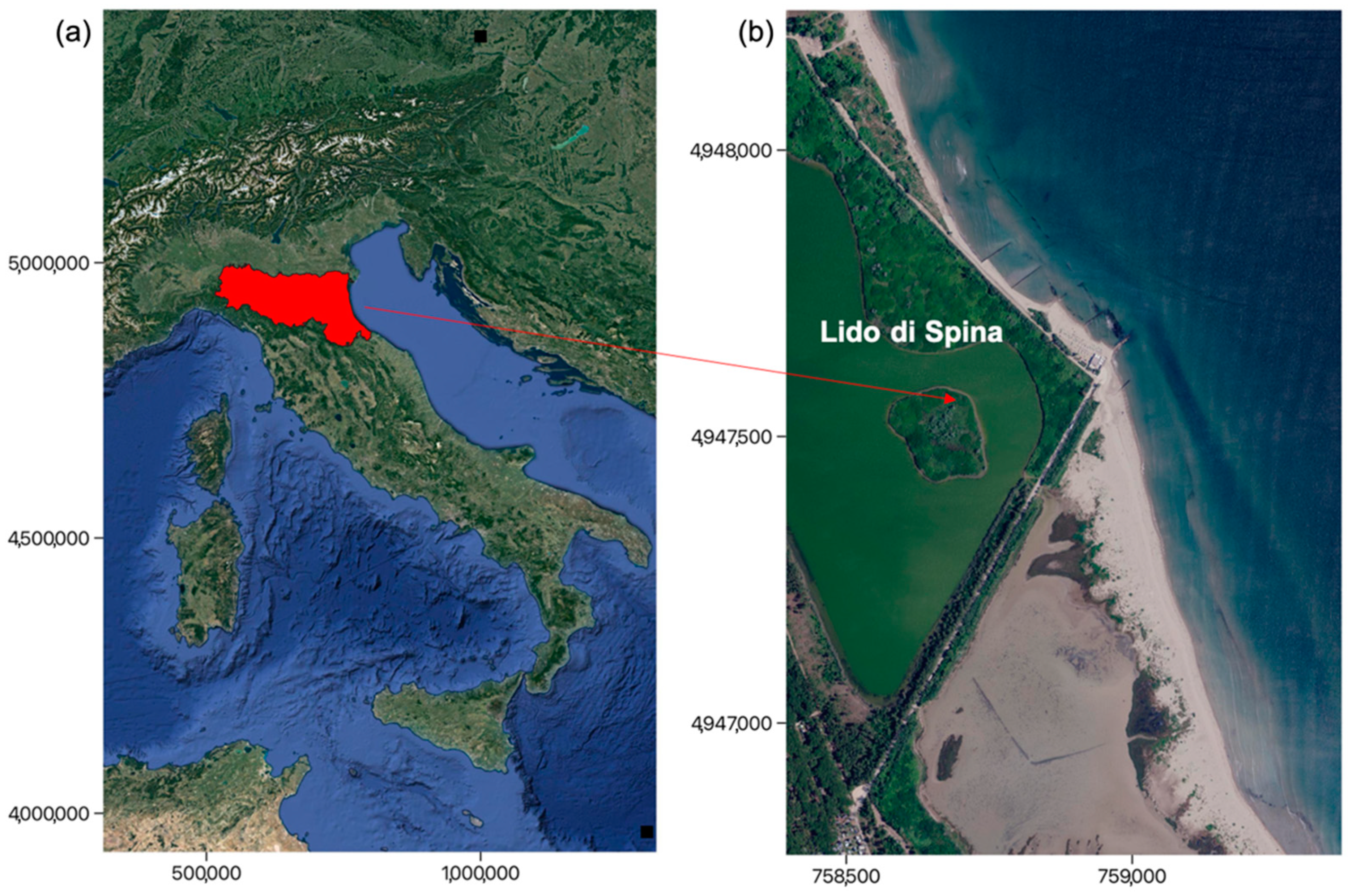
2. Study Area
3. Materials and Methods
3.1. Surveys Data
3.1.1. February 2019 Campaign
3.1.2. January–February 2020 Campaign
3.2. Pre Processed Data
3.3. Comparison Method
4. Results
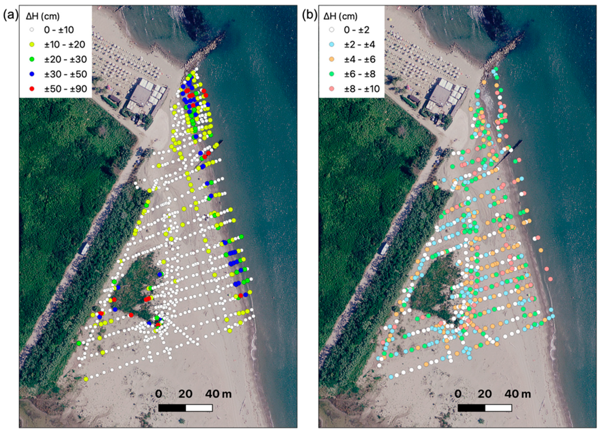
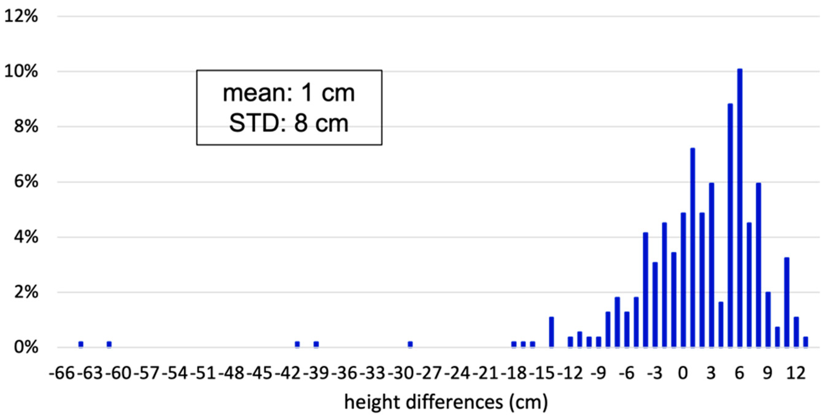
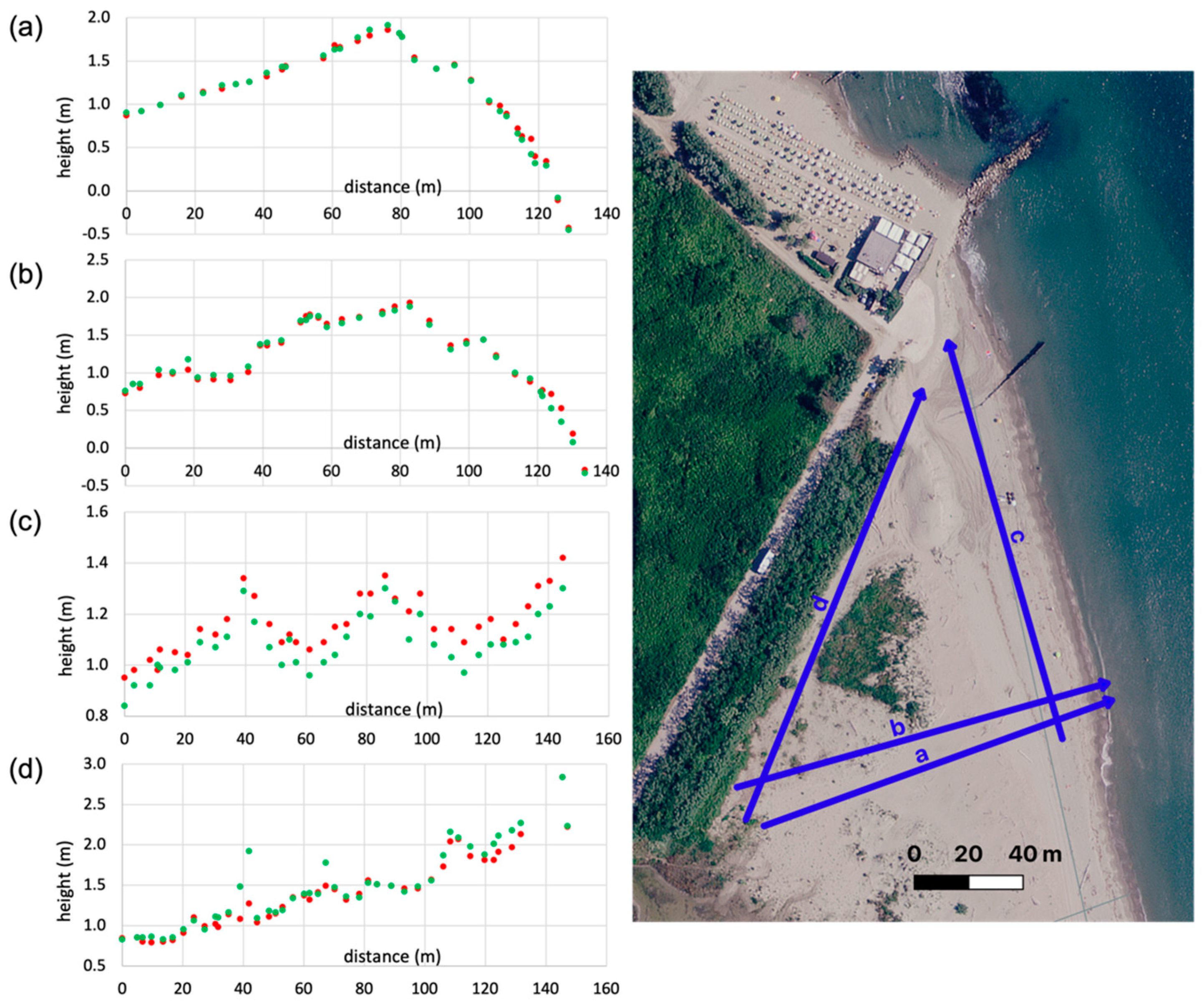
4.1. February 2019 Campaign
4.2. January–February 2020 Campaign
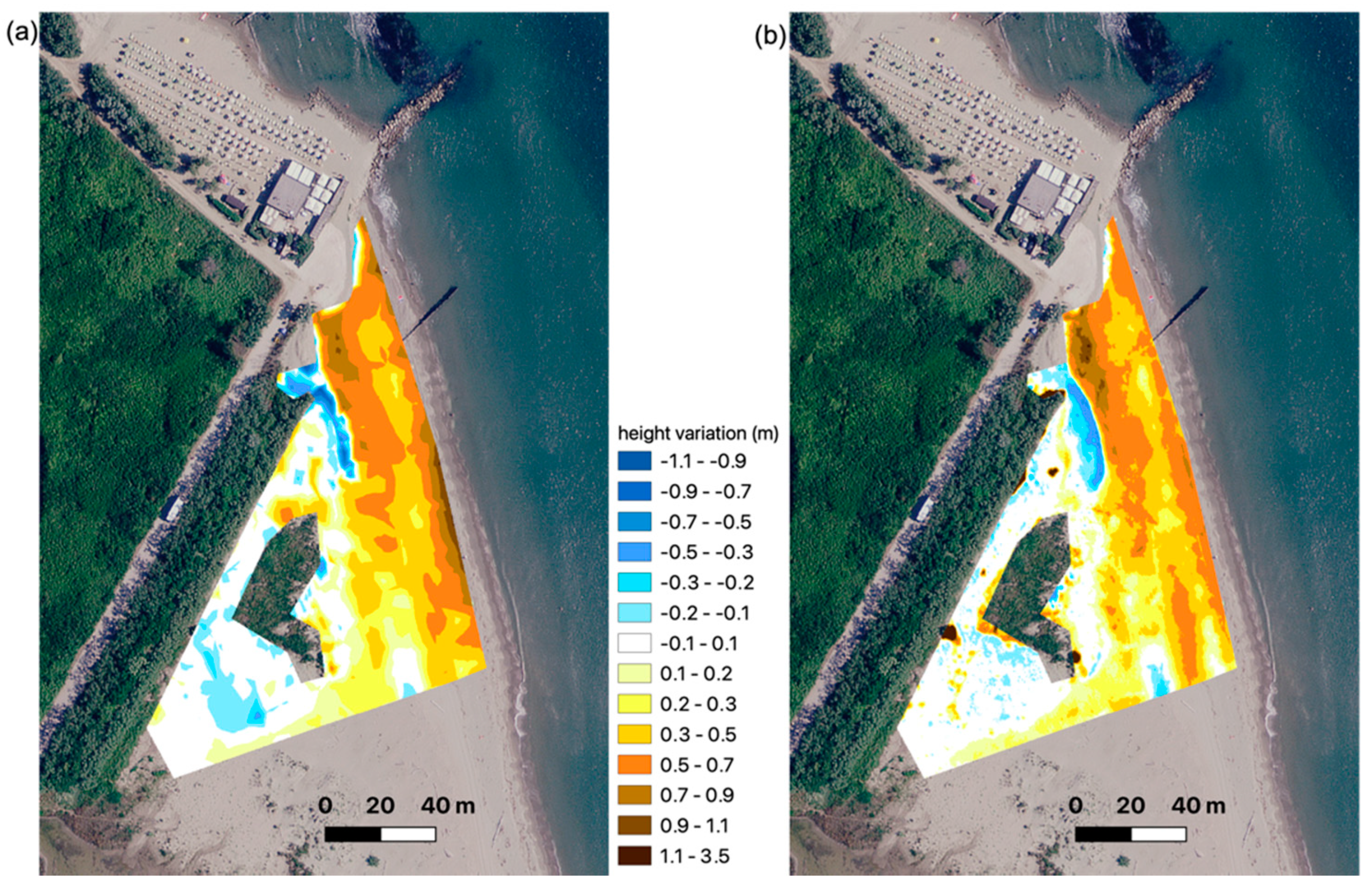
4.3. Volumes Monitoring
5. Discussion
6. Conclusions
Author Contributions
Funding
Conflicts of Interest
References
- Gonçalves, J.A.; Henriques, R. UAV photogrammetry for topographic monitoring of coastal areas. ISPRS J. Photogramm. Remote Sens. 2015, 104, 101–111. [Google Scholar] [CrossRef]
- Semeoshenkova, V.; Newton, A.; Contin, A.; Greggio, N. Development and application of an Integrated Beach Quality Index (BQI). Ocean Coast. Manag. 2017, 143, 74–86. [Google Scholar] [CrossRef]
- Duvat, V. Interest of quality-based policies for Integrated Coastal Zone Management implementation: Lessons learnt from a French case study. Ocean Coast. Manag. 2011, 54, 831–843. [Google Scholar] [CrossRef]
- Preti, M.; Zanuttigh, B.; De Nigris, N.; Martinelli, L.; Aguzzi, M.; Archetti, R.; Lamberti, A. Integrated beach monitoring at Igea Marina, Italy: Results of ten-years monitoring. Coast. Eng. Proc. 2011, 1, 199–226. [Google Scholar] [CrossRef] [Green Version]
- Perini, L.; Calabrese, L.; Salerno, G.; Luciani, P. Mapping of flood risk in Emilia-Romagna coastal areas. Nat. Hazards Earth Syst. Sci. Discuss. 2015, 3, 4315–4352. [Google Scholar]
- Gibbs, M. Coastal climate risk and adaptation studies: The importance of understanding different classes of problem. Ocean Coast. Manag. 2015, 103, 9–13. [Google Scholar] [CrossRef]
- Vecchi, E.; Aguzzi, M.; Albertazzi, C.; Nigris, N.D.; Gandolfi, S.; Morelli, M.; Tavasci, L. Third beach nourishment project with submarine sands along Emilia-Romagna coast: Geomatic methods and first monitoring results. Rend. Lincei Sci. Fis. E Nat. 2020, 31, 79–88. [Google Scholar] [CrossRef]
- Cohen, O.; Héquette, A. Recent Advances in Coastal Survey Techniques: From GNSS to LiDAR and Digital Photogrammetry-Examples on the Northern Coast of France. In Spatial Variability in Environmental Science-Patterns, Processes, and Analyses; IntechOpen: London, UK, 2020. [Google Scholar]
- Brunier, G.; Fleury, J.; Anthony, E.J.; Gardel, A.; Dussouillez, P. Close-range airborne Structure-from-Motion Photogrammetry for high-resolution beach morphometric surveys: Examples from an embayed rotating beach. Geomorphology 2016, 261, 76–88. [Google Scholar] [CrossRef]
- Pikelj, K.; Ružić, I.; Ilić, S.; James, M.R.; Kordić, B. Implementing an efficient beach erosion monitoring system for coastal management in Croatia. Ocean Coast. Manag. 2018, 156, 223–238. [Google Scholar] [CrossRef] [Green Version]
- Zanutta, A.; Lambertini, A.; Vittuari, L. UAV Photogrammetry and Ground Surveys as a Mapping Tool for Quickly Monitoring Shoreline and Beach Changes. J. Mar. Sci. Eng. 2020, 8, 52. [Google Scholar] [CrossRef] [Green Version]
- James, M.R.; Ilic, S.; Ruzic, I. Measuring 3D coastal change with a digital camera. Proc. Coast. Dyn. 2013, 24–28. Available online: https://xueshu.baidu.com/usercenter/paper/show?paperid=0290d01c329d043e494c14c39d6ef683&site=xueshu_se&hitarticle=1 (accessed on 24 October 2021).
- Gonçalves, R.M.; Awange, J.L. Three Most Widely Used GNSS-Based Shoreline Monitoring Methods to Support Integrated Coastal Zone Management Policies. J. Surv. Eng 2017, 143, 05017003. [Google Scholar] [CrossRef]
- Pitman, S.J.; Hart, D.E.; Katurji, M.H. Application of UAV techniques to expand beach research possibilities: A case study of coarse clastic beach cusps. Cont. Shelf Res. 2019, 184, 44–53. [Google Scholar] [CrossRef]
- Drummond, C.D.; Harley, M.D.; Turner, I.L.; A Matheen, A.N.; Glamore, W.C. UAV applications to coastal engineering. Eng. Aust. IPENZ 2015, 267–272. [Google Scholar] [CrossRef]
- Taddia, Y.; Corbau, C.; Zambello, E.; Russo, V.; Simeoni, U.; Russo, P.; Pellegrinelli, A. Uavs to assess the evolution of embryo dunes. In Proceedings of the International Archives of the Photogrammetry Remote Sensing and Spatial Information Sciences, Bonn, Germany, 4–7 September 2017; pp. 363–369. [Google Scholar]
- Milan, D.J.; Heritage, G.L.; Large, A.R.; Fuller, I.C. Filtering spatial error from DEMs: Implications for morphological change estimation. Geomorphology 2011, 125, 160–171. [Google Scholar] [CrossRef]
- Colomina, I.; Pere, M. Unmanned aerial systems for photogrammetry and remote sensing: A review. ISPRS J. Photogramm. Remote Sens. 2014, 92, 79–97. [Google Scholar] [CrossRef] [Green Version]
- Remondino, F.; Barazzetti, L.; Nex, F.; Scaioni, M.; Sarazzi, D. UAV photogrammetry for mapping and 3D modelling—Current status and future perspectives. ISPRS Int. Arch. Photogramm. Remote. Sens. Spat. Inform. Sci. 2011, 38, 25–31. [Google Scholar]
- Ružić, I.; Marović, I.; Benac, Č.; Ilić, S. Coastal cliff geometry derived from structure-from-motion photogrammetry at Stara Baška, Krk Island, Croatia. Geo-Mar. Lett. 2014, 34, 555–565. [Google Scholar] [CrossRef]
- Pajares, G. Overview and Current Status of Remote Sensing Applications Based on Unmanned Aerial Vehicles (UAVs). Photogramm. Eng. Remote Sens. 2015, 81, 281–329. [Google Scholar] [CrossRef] [Green Version]
- Turner, I.L.; Harley, M.D.; Drummond, C.D. UAVs for coastal surveying. Coast. Eng. 2016, 114, 19–24. [Google Scholar] [CrossRef]
- Jaud, M.; Grasso, F.; Le Dantec, N.; Verney, R.; Delacourt, C.; Ammann, J.; Deloffre, J.; Grandjean, P. Potential of UAVs for Monitoring Mudflat Morphodynamics (Application to the Seine Estuary, France). ISPRS Int. J. Geo-Inf. 2016, 5, 50. [Google Scholar] [CrossRef] [Green Version]
- Taddia, Y.; Stecchi, F.; Pellegrinelli, A. Coastal Mapping Using DJI Phantom 4 RTK in Post-Processing Kinematic Mode. Drones 2020, 4, 9. [Google Scholar] [CrossRef] [Green Version]
- Scarelli, F.M.; Sistilli, F.; Fabbri, S.; Cantelli, L.; Barboza, E.G.; Gabbianelli, G. Seasonal dune and beach monitoring using photogrammetry from UAV surveys to apply in the ICZM on the Ravenna coast (Emilia-Romagna, Italy). Remote Sens. Appl. Soc. Environ. 2017, 7, 27–39. [Google Scholar] [CrossRef]
- Mancini, F.; Dubbini, M.; Gattelli, M.; Stecchi, F.; Fabbri, S.; Gabbianelli, G. Using Unmanned Aerial Vehicles (UAV) for High-Resolution Reconstruction of Topography: The Structure from Motion Approach on Coastal Environments. Remote Sens. 2013, 5, 6880–6898. [Google Scholar] [CrossRef] [Green Version]
- Casella, E.; Rovere, A.; Pedroncini, A.; Stark, C.P.; Casella, M.; Ferrari, M.; Firpo, M. Drones as tools for monitoring beach topography changes in the Ligurian Sea (NW Mediterranean). Geo-Mar. Lett. 2016, 36, 151–163. [Google Scholar] [CrossRef]
- Andriolo, U.; Gonçalves, G.; Sobral, P.; Fontán-Bouzas, Á.; Bessa, F. Beach-dune morphodynamics and marine macro-litter abundance: An integrated approach with Unmanned Aerial System. Sci. Total Environ. 2020, 749, 141474. [Google Scholar] [CrossRef] [PubMed]
- Hoffmeister, D.; Tilly, N.; Curdt, C.; Aasen, H.; Ntageretzis, K.; Hadler, H.; Timo, W.; Andreas, V.; Georg, B. Terrestrial laser scanning for coastal geomorphologic research in western Greece. Int. Arch. Photogramm. Remote Sens. Spat. Inf. Sci. 2012, 39, 511–516. [Google Scholar] [CrossRef] [Green Version]
- Delacourt, C.; Allemand, P.; Jaud, M.; Grandjean, P.; Deschamps, A.; Ammann, J.; Cuq, V.; Suanez, S. DRELIO: An unmanned helicopter for imaging coastal areas. J. Coast. Res. 2009, 2, 1489–1493. [Google Scholar]
- Wheaton, J.M.; Brasington, J.; Darby, S.E.; Sear, D.A. Accounting for uncertainty in DEMs from repeat topographic surveys: Improved sediment budgets. Earth Surf. Process. Landf. J. Br. Geomorphol. Res. Group 2010, 35, 136–156. [Google Scholar] [CrossRef]
- Gandolfi, S.; De Nigris, N.; Morelli, M.; Tavasci, L.; Poluzzi, L.; Cenni, N. La Rete Geodetica Costiera della Regione Emilia-Romagna. ASITA 2017, 599–604. Available online: http://atti.asita.it/ASITA2017/ (accessed on 24 October 2021).
- Merloni, N. Gli habitat di interesse comunitario (Direttiva 92/43/CEE) nella Riserva Naturale Sacca di Bellocchio (province di Ravenna e Ferrara). Fitosociologia 2007, 44, 83–88. [Google Scholar]
- Merloni, M.; Piccoli, F. Comunità rare e minacciate dalle stazioni ravennati del Parco del Delta del Po. Fitosociologia 2007, 44, 67–76. [Google Scholar]
- Bertoni, D.; Armaroli, C.; Ciavola, P. Fast retreat of a barrier system due to reduced sediment supply (Bellocchio, Northern Adriatic Sea, Italy). In Proceedings of the 3rd CM2 Coastal Maritime Mediterranean Conference, Ferrara, Italy, 25–27 November 2015; pp. 7–10. [Google Scholar]
- Gaeta, M.G.; Bonaldo, D.; Samaras, A.G.; Carniel, S.; Archetti, R. Wave-2D Hydrodynamics Modeling at the Reno River Mouth (Italy) under Climate Change Scenarios. Water 2018, 10, 1380. [Google Scholar] [CrossRef] [Green Version]
- Aguzzi, M.; Costantino, R.; De Nigris, N.; Morelli, M.; Romagnoli, C.; Unguendoli, S.; Vecchi, E. Stato Del Litorale Emiliano-romagnolo al 2018: Erosione e Interventi di Difesa; ARPAE Emilia-Romagna: Emilia-Romagna, Italy, 2020; p. 224. [Google Scholar]
- Perini, L.; Lorito, S.; Calabrese, L. Il Catalogo delle opere di difesa costiera della Regione Emilia-Romagna. Studi Costieri 2008, 15, 39–56. [Google Scholar]
- Semeoshenkova, V.; Newton, A. Overview of erosion and beach quality issues in three Southern European countries: Portugal, Spain and Italy. Ocean. Coast Manag. 2015, 118, 12–21. [Google Scholar] [CrossRef]
- Van Rijn, L.C. Coastal erosion and control. Ocean Coast Manag. 2011, 54, 867–887. [Google Scholar] [CrossRef]
- Parisot, J.P.; Capo, S.; Castelle, B.; Bujan, S.; Moreau, J.; Gervais, M.; Réjas, A.; Hanquiez, V.; Almar, R.; Marieu, V. Treatment of topographic and bathymetric data acquired at the Truc-Vert Beach during the ECORS Field Experiment. J. Coast. Res. 2009, SI56, 1786–1790. [Google Scholar]


| Survey Data | 2019 | 2020 |
|---|---|---|
| Camera model | FC6310R | FC6310R |
| Resolution (px) | 5472 × 3648 | 5472 × 3648 |
| Focal length (mm) | 8 | 8 |
| Pixel size (µm) | 2.41 × 2.41 | 2.41 × 2.41 |
| N° frames | 563 | 638 |
| Flight altitude (m) | 104 | 108 |
| GSD (cm/px) | 2.87 | 2.64 |
Publisher’s Note: MDPI stays neutral with regard to jurisdictional claims in published maps and institutional affiliations. |
© 2021 by the authors. Licensee MDPI, Basel, Switzerland. This article is an open access article distributed under the terms and conditions of the Creative Commons Attribution (CC BY) license (https://creativecommons.org/licenses/by/4.0/).
Share and Cite
Vecchi, E.; Tavasci, L.; De Nigris, N.; Gandolfi, S. GNSS and Photogrammetric UAV Derived Data for Coastal Monitoring: A Case of Study in Emilia-Romagna, Italy. J. Mar. Sci. Eng. 2021, 9, 1194. https://doi.org/10.3390/jmse9111194
Vecchi E, Tavasci L, De Nigris N, Gandolfi S. GNSS and Photogrammetric UAV Derived Data for Coastal Monitoring: A Case of Study in Emilia-Romagna, Italy. Journal of Marine Science and Engineering. 2021; 9(11):1194. https://doi.org/10.3390/jmse9111194
Chicago/Turabian StyleVecchi, Enrica, Luca Tavasci, Nunzio De Nigris, and Stefano Gandolfi. 2021. "GNSS and Photogrammetric UAV Derived Data for Coastal Monitoring: A Case of Study in Emilia-Romagna, Italy" Journal of Marine Science and Engineering 9, no. 11: 1194. https://doi.org/10.3390/jmse9111194