Article

Investigation on Resistance, Squat and Ship-Generated Waves of Inland Convoy Passing Bridge Piers in a Confined Waterway

1
Research & Development Institute, Northwestern Polytechnical University, Shenzhen 518000, China
2
School of Marine Science and Technology, Northwestern Polytechnical University, Xi’an 710072, China
3
Roberval Laboratory, UT Compiègne-Sorbonne University, CS 60319, 60203 Compiègne, France
4
Cerema, CS 60039, 60200 Compiègne, France
5
ICUBE Laboratory, UMR 7357 CNRS, University of Strasbourg, 67000 Strasbourg, France
*
Author to whom correspondence should be addressed.
J. Mar. Sci. Eng. 2021, 9(10), 1125; https://doi.org/10.3390/jmse9101125
Submission received: 11 September 2021 / Revised: 8 October 2021 / Accepted: 11 October 2021 / Published: 14 October 2021
(This article belongs to the Special Issue Computational Fluid Mechanics)

Abstract

:
The average and unsteady hydrodynamics of an inland convoy passing bridge piers in a confined waterway were investigated using both numerical and experimental approaches. The numerical simulations are realized by solving the RANS (Reynolds-averaged Navier–Stokes) equations accounting for the solid body motion using the sliding mesh technique, while the experiments were carried out in the towing tank. The advancing resistance, trim, sinkage and ship-generated waves were analyzed as functions of the water depth, distance between bridge piers, draught and velocity. The existence of the piers is found to only influence the transient hydrodynamics of the convoy, but not the averaged properties. The ship-generated waves, especially the wave profiles at a specific lateral position, were characterized. Two wave crests exist at the pier position because of the additional reflections, creating a very complex wave pattern in the confined waterway.

1. Introduction

The interactions between ships and structures in water are of great importance, and include ship overtaking, passing moored vessels, crossing bridge piers, etc. They can influence the kinematic and kinetic properties of ships, and have to be considered during ship design and manufacture. When ships are maneuvered near these structures, special attention should be given to the rudder action and propulsion of the ship to avoid instabilities and possible collisions. Among these phenomena, the first three (ship encountering, overtaking, the passage of moored vessels) have been widely investigated [1,2,3,4,5,6], either by theoretical analysis, experiments or numerical simulations. However, the passage of bridge piers has not been studied in depth, but is equally important for ship navigation, especially in confined waters. Normally, there exist multiple bridge piers in water, which increase the restriction level of the waterway. When the distance between piers is very small (less than 4 times the ship breadth), this interaction becomes evident. Accidents are prone to happen at the pier position if the vessel is not properly controlled, causing damage to both the ship and bridge, especially in shallow waters. The hydrodynamics during the passage are therefore extremely significant to avoid accidents under these conditions.
Some work has been done to investigate the impact during a ship-bridge collision, with emphasis on the impact force of the collision and the damage [7,8,9,10,11,12,13,14,15,16]. However, the hydrodynamics during the passage are rarely investigated [17,18,19,20,21]. Tan and Gan [22] mathematically studied the influence of water level on ship-bridge collision. They concluded that the turbulence area near the bridge pier has a negative impact on safe passage. Li et al. [17] developed a 3-D Rankine boundary element method and simulated the unsteady hydrodynamic interaction during the process. A free surface re-meshing algorithm was proposed to treat the relevant moving boundary problem. The characteristics of the hydrodynamic loads were specified and the critical positions for the peak values have been identified. Zhang et al. [18] used a 3-D Rankine source boundary element method fully based on NURBS (non-uniform rational B-spline). The interaction forces and moments were numerically predicted. Zhang et al. [23] used CFD (computational fluid dynamics) techniques for this problem, where the unsteady viscous effect was considered. The transient forces and moments were predicted and the influence of the distance between the ship and the pier was analyzed. Xiang et al. [24] extended a method for evaluating the calm water-interacting loads with a submerged floating tube bridge up to the point of collision. Guo et al. [20] proposed an empirical formula relating to the minimum distance between the navigation ship and the bridge, which demonstrated that this distance increases logarithmically with flow velocity, and linearly with the pier’s diameter in the channel. Zheng [25] found that pier scouring made the bending moments of pier bodies increase under the same ship impact force and the reduction effect of the ship impact resistance force on piers by scouring cannot be ignored. Khangaonkar et al. [21] presented an assessment of zone of influence (ZOI) from the Hood Canal Bridge in the Salish Sea, Washington. The results confirmed that this bridge obstructs the brackish outflow surface layer, which induces increased local mixing near the bridge, causes pooling of water (up-current) during ebb and flood, and results in shadow/sheltering of water (down-current). The study of this phenomenon is still worthy, which is promising to uncover the unsteady hydrodynamic process and give useful insights and suggestions for ship maneuvering actions.
In this study, an inland convoy passing bridge piers was simulated using CFD methods to investigate the influence of the piers on the inland convoy in a confined waterway. The advancing resistance, squat and wave patterns are analyzed and characterized.

2. Numerical and Experimental Details

2.1. Governing Equations Accounting for Solid Body Motions
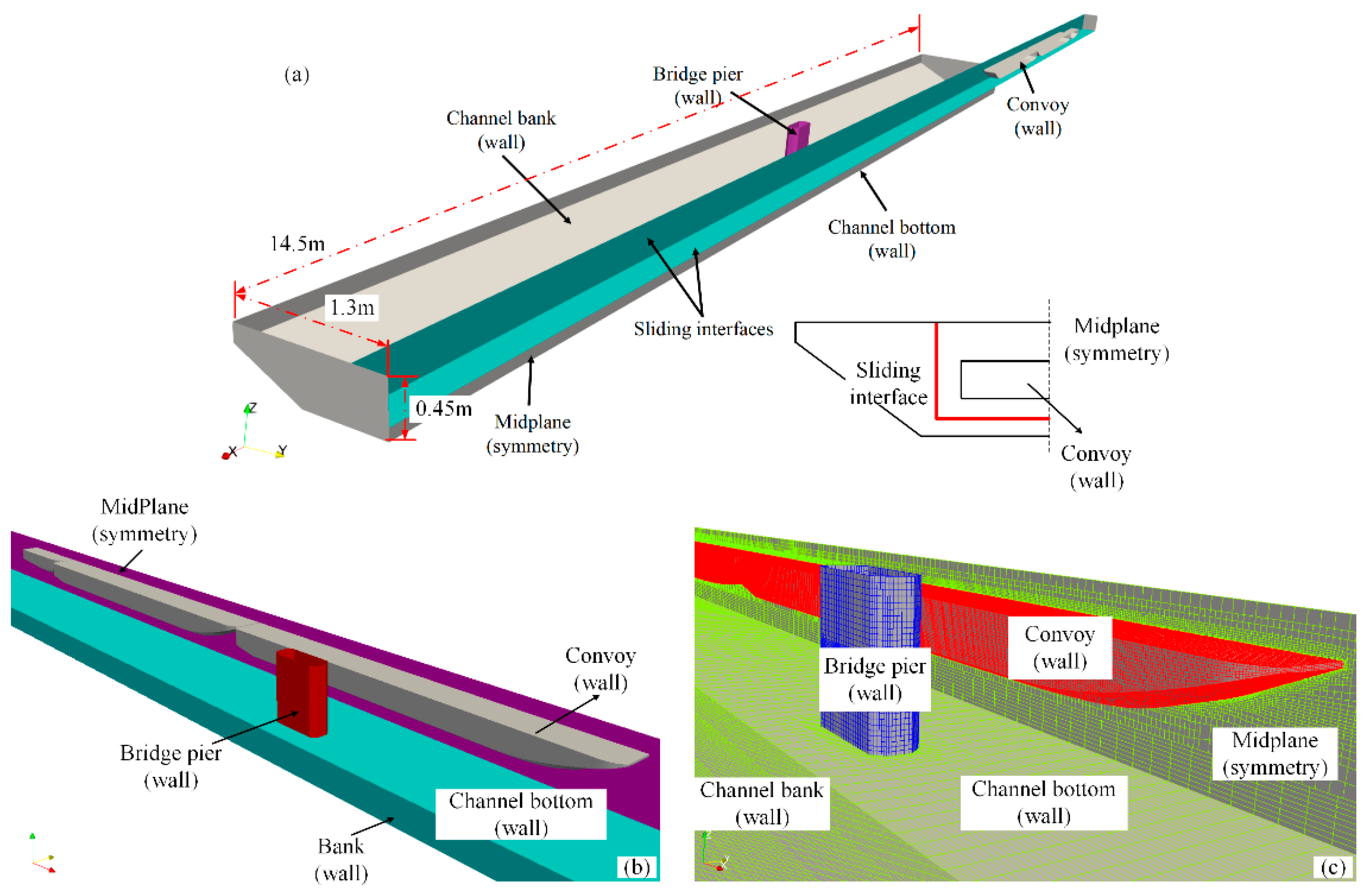
The governing equations of fluid flow (RANS) are as follows [26,27]:
u = 0 ,
u t + ( u u ) = p ρ + ( ν e f f u ) + g + f σ ,
where u , ρ and p are the velocity, density and pressure of the fluid. The fluid is treated as incompressible ( ρ = const ). The open-source code OpenFOAM is used throughout this work. The pressure and velocity are decoupled using the merged-PISO-SIMPLE scheme, which allows larger time steps and thus accelerates the simulations. ν e f f = ν + ν t is the effective dynamic viscosity, consisting of the fluid viscosity ( ν ) and the eddy viscosity ( ν t ) calculated from a certain turbulence model. The S S T   k ω model is adopted in this study. It is a two-equation eddy-viscosity model which combines the advantages of the k ϵ and k ω models. The k ω model is used in the boundary layer and the k ϵ model is used in the free stream flow. Thereby it is less sensitive to free stream conditions and has better performance predicting the flow separation and reattachment. Different turbulence models, including the k ε , k w and S S T   k ω models, were all tested as in Figure 1. It can be observed that the S S T   k ω model produces the most accurate resistance coefficient among them. The S S T   k ω model was ultimately selected, on account of its precision performance.
The VOF (volume-of-fluid) model is adopted to capture the free surface between water and air:
α t + ( α u ) + [ α ( 1 α ) u r ] = 0 ,
where u r is the compressive velocity field acting in the normal direction towards the interface. α = V w / V is the phase fraction, also called the indicator function, where V w is the volume of water inside a control volume V. The VOF method is conservative because α is bounded between 0 and 1. α = 0 and α = 1 correspond with air and water. The last term of Equation (3) can prevent excessive smearing of the free surface.
When the solid in the computational domain moves, the surrounding cells should also be moved to maintain their shapes, i.e., the mesh quality. The grid velocity u g should thus be added into the momentum Equation (2) through the ALE (arbitrary Lagrangian–Eulerian) approach:
u t + ( ( u u g ) u ) = p ρ + ( ν e f f u ) + g + f σ ,
where the grid velocity u g can be determined by the space conservation law:
t V d V S u g d S = 0 ,
During the simulation, the sliding mesh technique is utilized to account for the process of the convoy passing the bridge piers. Interfaces are created between the domains of the convoy and the piers. The adjacent mesh domains exchange information through interpolation at the interfaces. Each cell face of the local patch (slave patch) accepts contributions from the overlapping faces of the neighbor patch (master patch) at the sliding interface, with the weights defined as a fraction of the intersecting areas. For each face, the sum of the weights should be 1. Interpolation weights at the interface are constructed such that the interpolation results in conservation. Conservation errors are introduced as the sum of weights deviates from 1 where the patch geometries are not well matched. Consistent and conservative discretization across the interface is achieved using weighted interpolation [29,30].
For the flow variables from the master patch to the slave patch [31]:
ϕ S i = n W M n S i ϕ M n ,
where ϕ and W denote the flow variable and the weight. The subscripts ’M’ and ’S’ represent the master and slave patches, respectively. It can be observed that the value of the flow variable at the slave patch is calculated from the weighted sum of that at the master patch.
For the ones from the slave patch to the master patch:
ϕ M j = m W S m M j ϕ S m ,
in order for the interface discretization to remain conservative, the following three constraints are obeyed:
W M n S i = 1.0 ,
W S m M j = 1.0 ,
W M n S i | S M n | = W S m M j | S M j | = | S M S | ,
with the additional symmetry constraint:
W M n S i > 0     W S i M n > 0 ,
where ϕ S and ϕ M are the variables of the slave and master patch, respectively. i and j denote the ith and jth facets at the slave and master patches. n is the number of master facets neighboring the slave facet i, and m is the number of the slave facets neighboring the master facet j. W M S and W S M are the master-to-slave and slave-to-master weighting factors, respectively. | S M | , | S S | and | S M S | are the surface area of the master facet, the surface area of the slave facet and the intersection between the master and slave facets, respectively.
The value of the weighting factors is basically the percentage of the surface intersection between two overlapping facets deduced from Equation (10):
W M S i = | S M S i | | S M n |     [ 0.0 , 1.0 ] ,
W S M i = | S S M j | | S S n |     [ 0.0 , 1.0 ] ,
Because of the domain discretization, the two meshes may not overlap with each other, making the weighting factors underestimated (smaller than 1.0), i.e., the simulation will not be conservative. It is therefore suggested to use enough mesh resolution at the interface and use similar mesh sizes between the master and slave patches for the sake of accuracy. If this cannot be satisfied, remedies can be adopted. Corrections for low weight are used here, which rescale the face weighting factors so they will sum up to 1.0. For each neighboring face involved, the rescaling will be proportional to the initial value of the neighbor face weighting factor, so the overall correction for each face ends up being weight interpolated.

2.2. Testing Setups

The experiments were carried out in the ANAST laboratory of the University of Liège. The testing setup and parameter definitions can be found in Figure 2. The towing tank was adjusted with trapezoidal banks with a slope of 2:1, resembling the real conditions of an inland waterway. Two bridge piers were designed and placed symmetrically in the channel. An inland convoy model with one pusher and one barge was used with the scale ratio 1/25, according to the dimension of the towing tank. The length of the convoy in model scale was 7.0 m. This convoy is widely-used during inland waterway transport in Europe. In the experiments, the convoy model was towed by the carriage with a specific velocity. It passed through the space between the piers, which are composed of two concrete blocks with the dimensions 40   cm × 16   cm . A six-component dynamometer balance was used to measure the forces and moments on the vessel. The system was calibrated before the experiments, with reported uncertainty of 8% for the force. More details about the experiments can be found in [32,33].
The computational domain was designed as the experiments in Figure 2. The length of the channel was 14.5 m. Since the domain is symmetrical in the y direction, only one-half was simulated with the symmetry boundary condition to reduce the grid number. The boundary conditions and principal dimensions of the domain are denoted in the figure. The advective boundary condition was adopted to avoid wave reflections at both ends of the channel. The sliding interfaces were designed between the convoy and the bridge pier/channel bottom [6]. The area near the pier is zoomed in Figure 3b to demonstrate their relative position. The computational mesh is shown in Figure 3c. The areas of the convoy, free surface and the bridge pier are clearly refined to capture the complex flow and accurately calculate the forces. Boundary layers were added near the hull with the dimensionless wall distance y + being about 60. The converged solution of a towed case was used as an initial condition to reduce the influence of the impulsive start.
The channel dimensions and testing conditions were designed as in Table 1. All tests were performed with the channel bottom width 1.44 m. Two pier distances, two draughts, three water depths and several velocities were tested during the simulations and experiments. The maximum Froude number was 0.738, which means that all our tests were in sub-critical conditions ( F r h < 1 ). The initial position of the convoy was placed 6.5m away from the pier to guarantee the fully-developed wakes generated by the vessel. The vessel took about 16~18 s to finish the whole passing process in the current domain. The dimensions of the channel and pier resemble real conditions during inland waterway transport. The mesh was generated using the snappyHexMesh utility in OpenFOAM. The mesh numbers can be found in Table 1.
Verification and Validation (V & V) studies were carried out in advance using the standard hull forms KCS and KVLCC2. A grid convergence study with three mesh resolutions and a time step convergence study with four timesteps were performed to select appropriate mesh generation strategy and time steps. The resistance was also validated with the ITTC benchmarks. Details of the grid and the time step independence study can be found in our earlier work [34]. The accuracy of the simulation can thus be guaranteed. A fixed time step of 0.001s was selected in this work.
During the solution of the RANS equations, the time derivative term was discretized using the implicit Euler scheme. The convection terms in the momentum and VOF equations were discretized with the second-order linear upwind scheme and the second-order TVD (total variation diminishing) scheme with van Leer’s flux limiter. The diffusion term was discretized by a second order central differencing scheme with non-orthogonal correction. Five outer corrections and two pressure corrections were employed for the velocity–pressure coupling. All equations were solved to the tolerance of O ( 8 ) [35,36]. Each case used 52 processors and takes about 12 CPU hours to finish. The actual physical time was about the same level.
To characterize the process of the convoy passing bridge piers, a parameter ξ s b similar to that of ship–ship interaction is defined in this study.
ξ s b = x s b / L m ,
where ξ s b is the longitudinal distance between the convoy and the bridge pier. L m = ( L s + L b ) / 2 is the average length of the convoy and the pier. The unsteady forces and wave changes can then be characterized as functions of the relative position between the amidships of the convoy and the pier. Figure 4 demonstrates the three most important positions of the passing process. When ξ s b = 1 , the convoy meets the piers. When ξ s b = 0 , the centers of the convoy and the pier are located at the same longitudinal position. When ξ s b = 1 , the passing ends. The positions within 1 < ξ s b < 1 are important for the transient properties of the convoy.

3. Results and Discussions

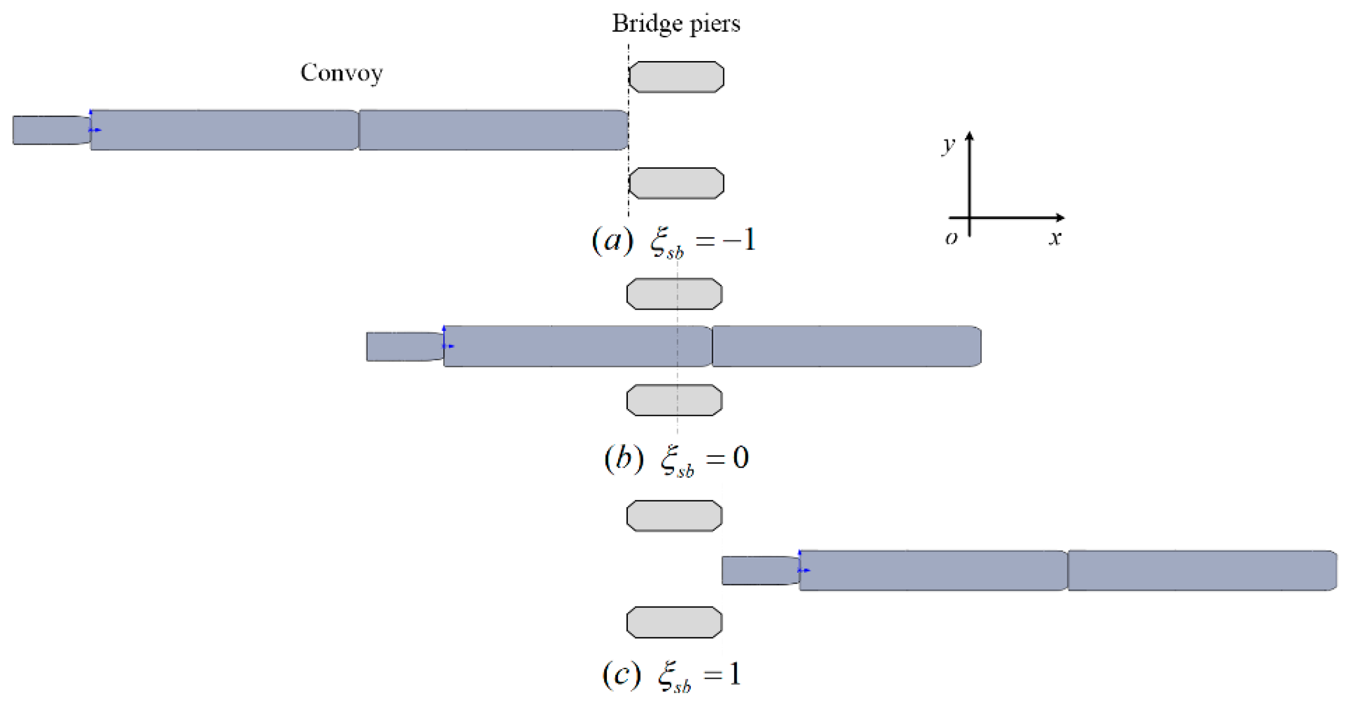
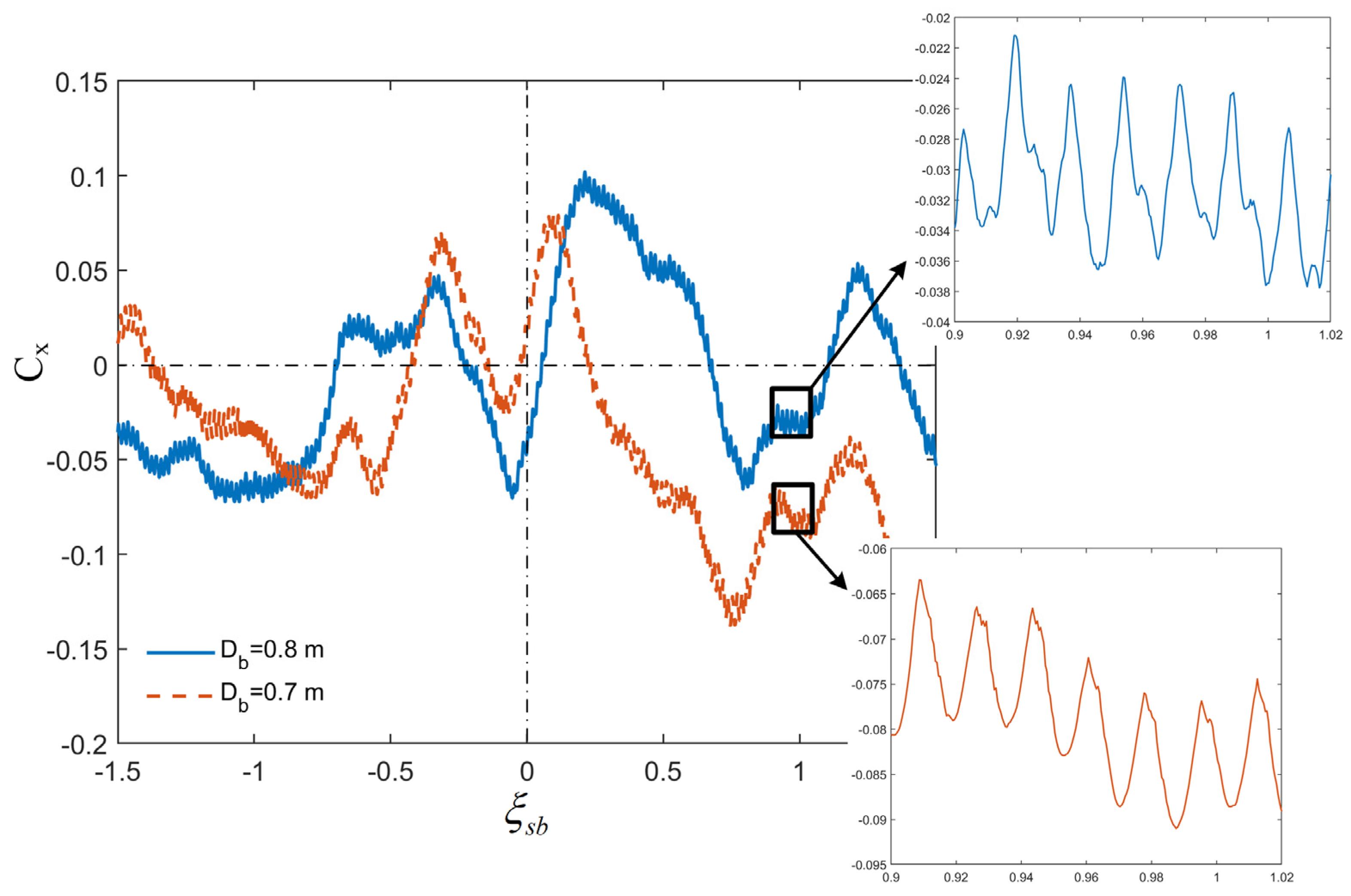
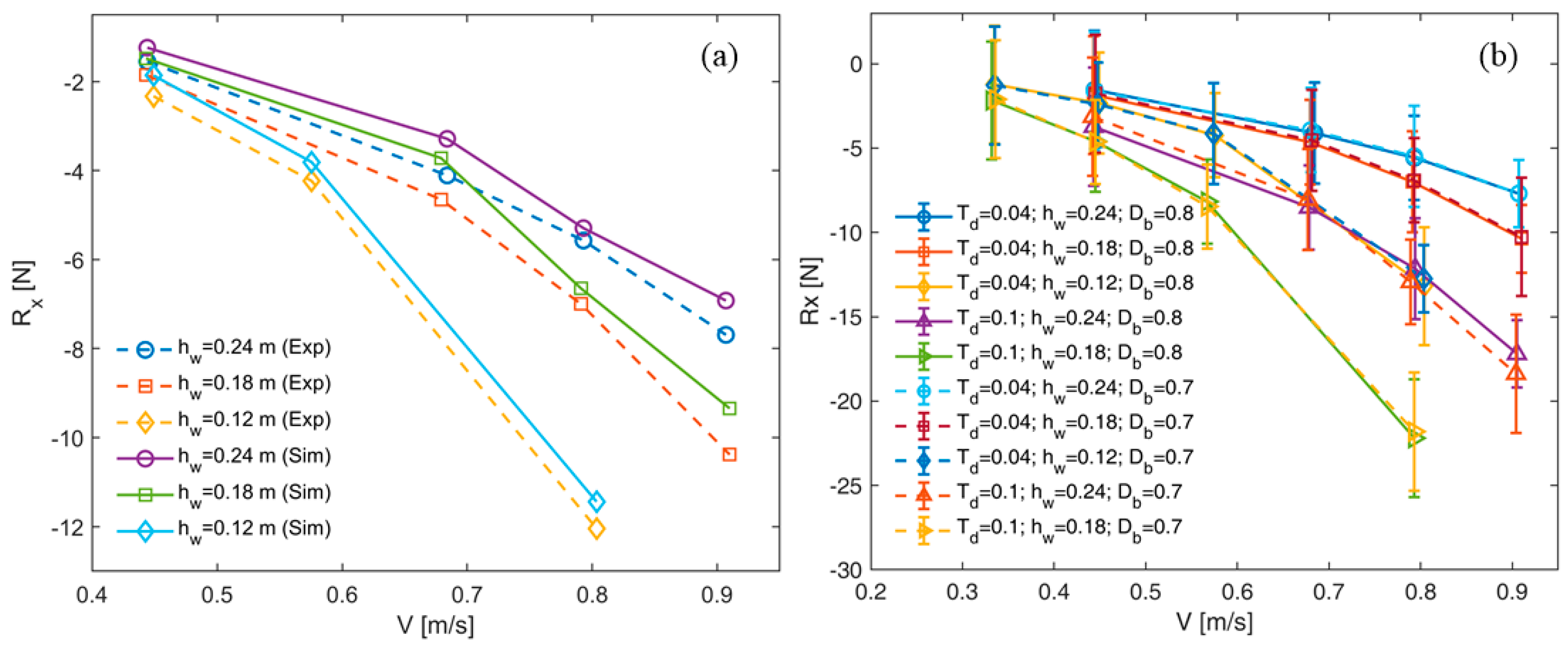
3.1. Advancing Resistance during the Convoy Passing Bridge Piers

The transient effects while the convoy is passing bridge piers are significant since they may change the unsteady hydrodynamics and maneuverability during the crossing. The instantaneous resistance coefficient ( C x = R x 1 2 ρ v 2 B T , B and T are the width and draught of the vessel) is plotted against the relative position ( ξ s b ) in Figure 5 as a function of the pier distance, with two smaller windows showing a shorter period of time. To concentrate on the transient process, the average value is removed from the resistance directly obtained from the simulations. With a smaller pier distance, the oscillation of the resistance is stronger since the space restriction is increased. The force oscillation mainly lies in the range of 1 < ξ s b < 1 . The resistance changes intensively near the position ξ s b = 0 where the centers of the convoy and the piers coincide during the passing process. This means that the convoy experiences the strongest time-varying interactions with the piers at this position, to which attention should be paid during real maneuvering. Similar trends can be found in Figure 6 as a function of the water depth. The oscillation is higher with a smaller water depth. However, slight unsteady effects can also be observed when ξ s b < 1 and ξ s b > 1 . This can be caused by the disturbances introduced by the evolution of the system, because the initial conditions may not be realistic at the beginning.
The average resistance during the passing process is measured in the experiment. In Figure 7a, the simulated values are compared with the experiments. The direction of the convoy advancement is defined as positive, which is the reason why the resistance values are all negative in the results. The simulations agree with the experimental data, but the resistance was underestimated. The largest error between the two was about 7%. This means that our simulations can predict the unsteady process with acceptable accuracy.
All the advancing resistances with various water depths, pier distances, draughts and velocities are demonstrated in Figure 7b. Clearly, the resistance increases with the convoy velocity and draught. With the decrease of the water depth, the advancing resistance increases because of the enhancement of the confinement level, which makes the convoy consume more fuel and increases the difficulty of ship maneuvering. When the water depth is too small, the possibility of grounding also increases. This relates to the squat effect, a combination of trim and sinkage, which will be analyzed later. Similar to the water depth, the resistance is reckoned to increase with the decrease of the pier distance, which also increases the confinement of the waterway. However, this is not evident in the figure. The distance between the bridge piers does not seem to influence the average resistance of the convoy. The bridge piers do increase the confinement, however, because of their small size, their influences are temporary and instantaneous. The unsteady effect of the passing process will counteract it. Therefore, the appearance of structures near the convoy only influences transient properties, but not averaged ones, which means that the overall fuel consumption is not affected by the passing process.

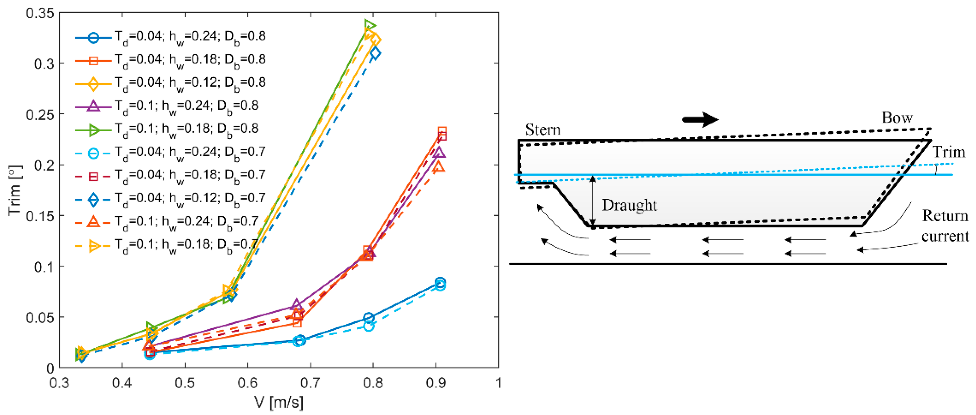
3.2. Trim and Sinkage Analysis

Squat is caused by the overall reduction in under keel clearance (UKC) forward or aft between a convoy at rest and underway due to the accelerated flow around the moving body [37,38,39,40]. It greatly influences resistance and maneuverability. In shallow water, a large squat can lead to grounding, posing potential dangers to the ship navigation. Squat is actually the combination of the trim and sinkage of the convoy. As the resistance, averaged trim and sinkage values are plotted against the water depth h w , distance between bridge piers D b , draught T d and velocity V. Their definitions can be observed in Figure 8 and Figure 9. The trim is defined as the pitch angle underway. It can be seen that the trim increases with the augmentation of the draught and velocity, and the reduction of the water depth. The same trend can be observed for the sinkage. However, the distance between the bridge piers does not influence the averaged properties. The trim and sinkage are caused by the return current around the convoy. When the space is restricted, the flow there will be accelerated, which leads to pressure reduction. Thus, an attracting force to the nearest wall is generated, causing the so-called sinkage. Because of the flow direction and the hull form, the motions of the bow and stern are different, a pitching moment is also generated; the trim then appears.

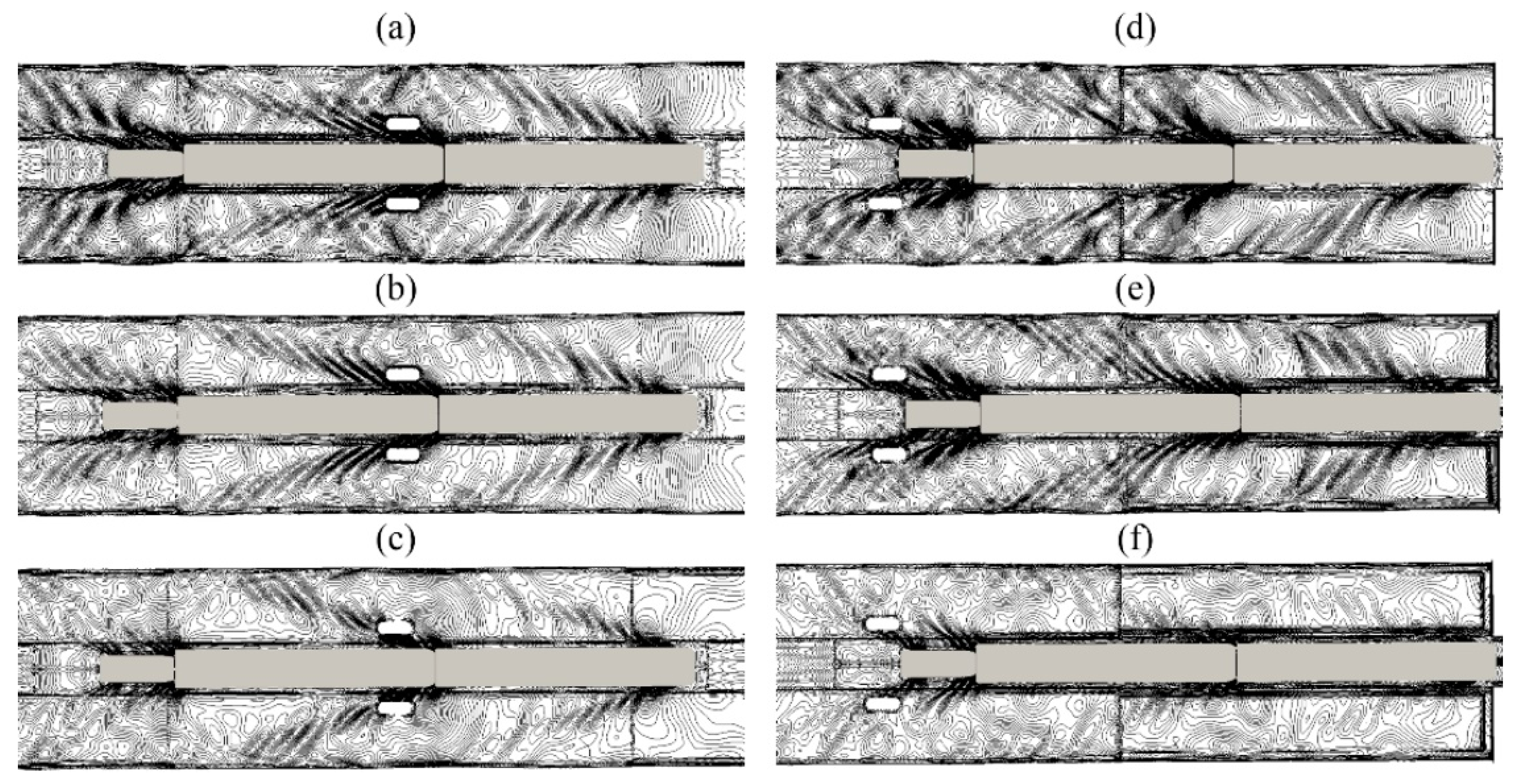
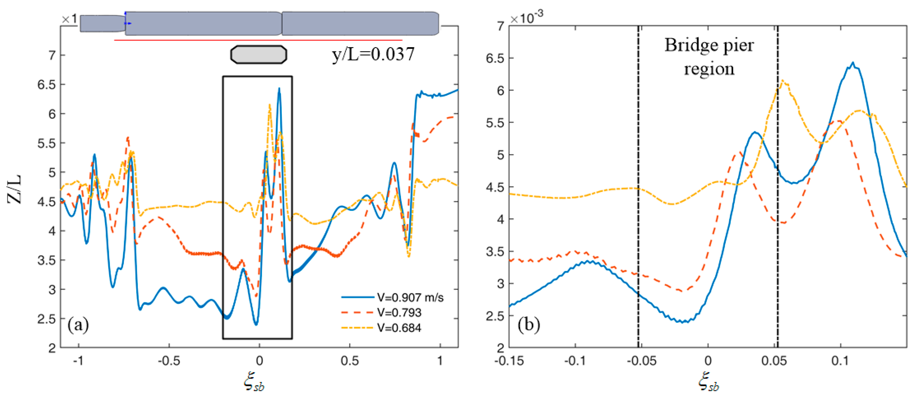
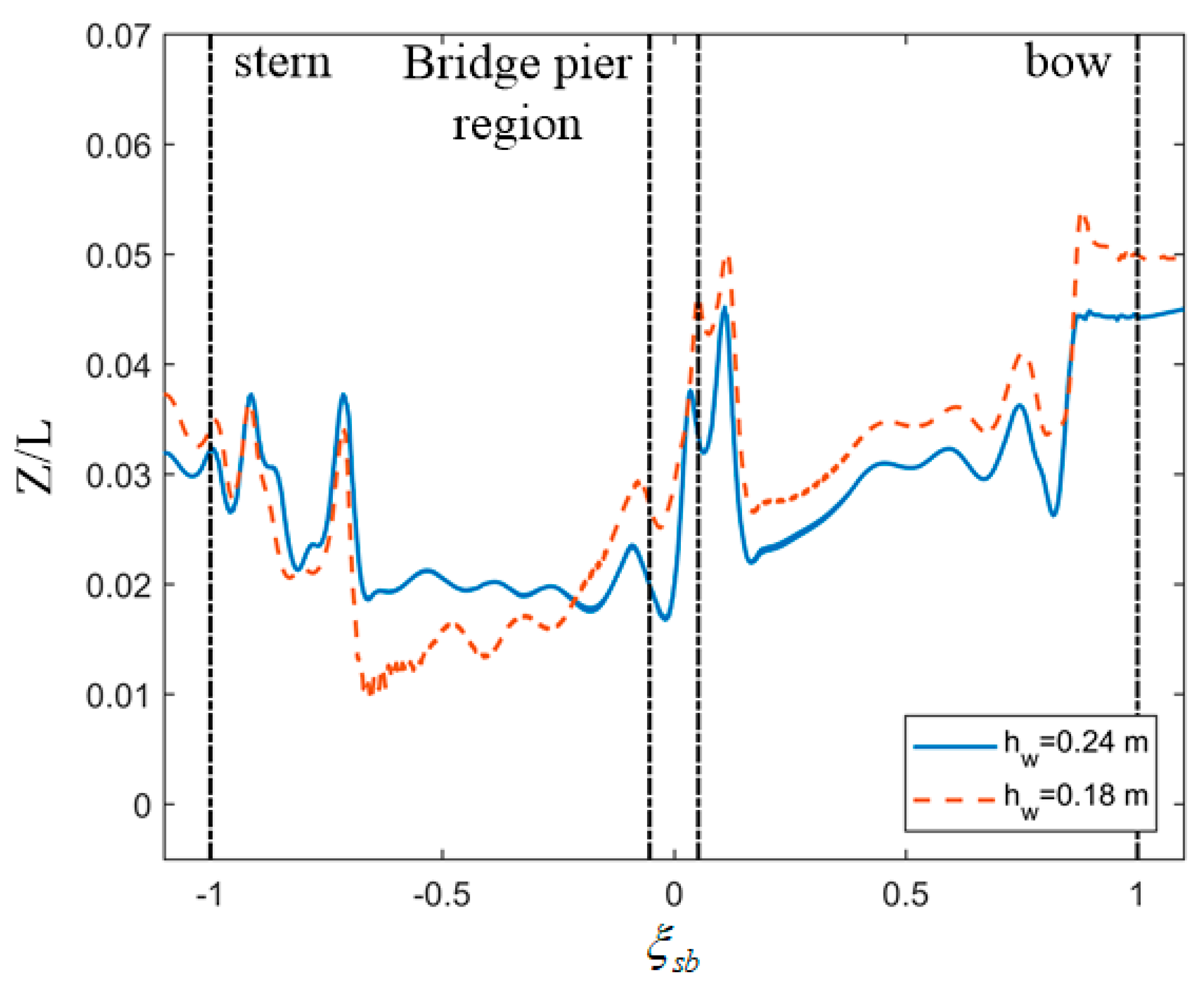
3.3. Ship-Generated Waves Influenced by Bridge Piers

The appearance of the bridge piers will inevitably influence the wave pattern generated by the convoy. The ship waves with different speeds are shown in Figure 10, and were well captured by our simulations. Two important positions with ξ s b = 0 and ξ s b = 1 are demonstrated. The traditional Kelvin wave pattern can be clearly observed [41]. The waves generated by the bows of the two barges and the pusher are the most evident. Because of the bank, the waves are reflected and then superposes with the original ones, creating a very complicated wave pattern. With a higher velocity, the wave change becomes more intensive, which can be observed by the isolines in the figure. It is clear that the wave fields are disturbed by the bridge piers. To quantitatively characterize the wave properties, the wave profiles at the lateral position y / L = 0.037 (the center between the convoy and the bridge pier) are extracted for comparison in Figure 11. The overall ship waves are lower than the initial water level. The wave crests originate from the bows and sterns. A larger speed makes the wave profile higher in front of the convoy and lower in the middle. The wave change is more violent with a higher convoy velocity. At the position of the pier, two wave crests were observed. The waves there are zoomed in Figure 11b. It can be seen that this is caused by the wave reflection of the pier, which further superimposed with the original wave pattern. Because of the restricted space, the wave change becomes more intensive.
Figure 12 demonstrates the influence of water depth. The wave contours are different for the two water depths, especially near the pusher. The waves created by the two barges finally superimpose with the pusher waves and form a very complex wave pattern. The influence becomes clearer in the extracted wave profiles in Figure 13. The positions of the wave crests remain the same. With a smaller water depth and pier distance, the wave elevation becomes higher because of the space restriction. The water level is more easily influenced by the channel bottom when the water depth is lower, creating a more deformed wave pattern.
The influence of the pier distance can be found in Figure 14. Since the pier distances are small, no significant differences can be observed. However, they are evident enough in the extracted profiles (Figure 15). The pier will create a more confined condition beside the channel, and the water level will be elevated. A smaller pier distance will create a more confined condition, which will make the water level higher. Nevertheless, the pier distance will not influence the overall wave pattern because the wave crests and troughs are at the same positions. This is also the reason why no significant differences can be seen in Figure 14.

4. Conclusions

During inland shipping, vessels will inevitably pass bridges, where the bridge piers exert stronger confinement apart from the channel banks. The ship dynamics and maneuverability change during this process. In this study, the hydrodynamics including the advancing resistance, trim, sinkage and ship-generated waves of the inland convoy passing the bridge piers in a confined waterway were investigated using the CFD and experimental approaches. The RANS equations were solved during the numerical simulations, using the sliding mesh technique for the motion of the convoy. The experiments were carried out in the towing tank of the ANAST laboratory in the University of Liège.
The averaged and transient resistances were both analyzed as functions of water depth, pier distance, draught and velocity. The averaged values agree well between simulations and experiments. The averaged resistance was found to increase with the increase of the draught and velocity and the decrease of the water depth. The influence of the bridge piers on the mean properties is not evident, since the averaged resistance does not change with the distance between the piers according to our results. In reality, this means that the fuel consumption remains the same with or without the bridge piers. However, the appearance of the piers has great influence on the transient properties of the convoy. A parameter of the relative position between the convoy and the pier was defined to characterize the crossing process. The fluctuation of the resistance during the procedure clearly increased when the space restriction of the piers increased.
The increase of the squat may lead to grounding. To characterize the squat in a confined waterway, the trim and sinkage were first analyzed as functions of the water depth, pier distance, draught and velocity. The averaged characteristics were emphasized here. Similar conclusions with the resistance can be drawn for the averaged squat.
The ship-generated waves were successfully captured by our simulations. Wave crests were found to originate from the bow and stern. In a confined waterway where both sides and the bottom are restricted, the ship waves are reflected at these positions, and further superpose with the original ones, creating a very complex wave pattern in the waterway. When influenced by the bridge piers, the waves will reflect once more, leading to the appearance of two wave crests near the pier.
As a result, the averaged and transient parameters were analyzed for a convoy passing bridge piers. The wave pattern near the bridge pier was analyzed to characterize the flow fields. These data provide insights into this phenomenon and can be used for their further predictions.

Author Contributions

Conceptualization, P.D. and A.O.; methodology, P.D.; software, P.D.; validation, P.D.; formal analysis, P.D., A.O., Y.H. and H.H.; investigation, P.D., A.O. and H.H.; resources, P.S.; data curation, P.D.; writing—original draft preparation, P.D.; writing—review and editing, P.D., Y.H. and H.H.; visualization, P.D.; supervision, A.O. and P.S.; project administration, A.O. and P.S.; funding acquisition, P.D. and A.O. All authors have read and agreed to the published version of the manuscript.

Funding

This research was funded by the Guangdong Basic and Applied Basic Research Foundation (Grant No. 2019A1515110863), Fundamental Research Funds for the Central Universities (Grant No. 3102020HHZY030004, 3102019JC006), National Natural Science Foundation of China (Grant No. 51979226, 52171324), Natural Science Basic Research Program of Shaanxi (Program No.2020JC-18) and Shaanxi Provincial Key R&D Program (2021KW-38).

Conflicts of Interest

The authors declare no conflict of interest.

References

  1. Xie, N.; Iglesias, G.; Hann, M.; Pemberton, R.; Greaves, D. Experimental study of wave loads on a small vehicle in close proximity to a large vessel. Appl. Ocean Res. 2019, 83, 77–87. [Google Scholar] [CrossRef]
  2. Xu, H.F.; Zou, L.; Zou, Z.J.; Yuan, Z.M. Numerical study on hydrodynamic interaction between two tankers in shallow water based on high-order panel method. Eur. J. Mech. B Fluids 2019, 74, 139–151. [Google Scholar] [CrossRef] [Green Version]
  3. Gourlay, T. Sinkage and trim of two ships passing each other on parallel courses. Ocean Eng. 2009, 36, 1119–1127. [Google Scholar] [CrossRef] [Green Version]
  4. Wang, J.; Zou, L.; Wan, D. Numerical simulations of zigzag maneuver of free running ship in waves by rans-overset grid method. Ocean Eng. 2018, 162, 55–79. [Google Scholar] [CrossRef]
  5. Mousaviraad, S.M.; Sadat-Hosseini, S.H.; Carrica, P.M.; Stern, F. Ship–Ship interactions in calm water and waves. Part 2: URANS validation in replenishment and overtaking conditions. Ocean Eng. 2016, 111, 627–638. [Google Scholar] [CrossRef] [Green Version]
  6. Wang, H.Z.; Zou, Z.J. Numerical study on hydrodynamic interaction between a berthed ship and a ship passing through a lock. Ocean Eng. 2014, 88, 409–425. [Google Scholar] [CrossRef]
  7. Wuttrich, R.; Wekezer, J.; Yazdani, N.; Wilson, C. Performance Evaluation of Existing Bridge Fenders for Ship Impact. J. Perform. Constr. Facil. 2001, 15, 17–23. [Google Scholar] [CrossRef]
  8. Wang, L.; Yang, L.; Tang, C.; Zhang, Z.; Chen, G.; Lu, Z. On the Impact Force and Energy Transformation in Ship-Bridge Collisions. Int. J. Prot. Struct. 2012, 3, 105–120. [Google Scholar] [CrossRef]
  9. Wang, L.; Yang, L.; Huang, D.; Zhang, Z.; Chen, G. An impact dynamics analysis on a new crashworthy device against ship-bridge collision. Int. J. Impact Eng. 2008, 35, 895–904. [Google Scholar] [CrossRef]
  10. Svensson, H. Protection of bridge piers against ship collision. Steel Constr. 2009, 2, 21–32. [Google Scholar] [CrossRef]
  11. Zhi-Qiang, H.; Yong-Ning, G.; Zhen, G.; Ya-Ning, L. Fast evaluation of ship-bridge collision force based on nonlinear numerical simulation. J. Mar. Sci. Appl. 2005, 4, 8–14. [Google Scholar] [CrossRef]
  12. Fan, W.; Liu, Y.; Liu, B.; Guo, W. Dynamic Ship-Impact Load on Bridge Structures Emphasizing Shock Spectrum Approximation. J. Bridg. Eng. 2016, 21, 04016057. [Google Scholar] [CrossRef]
  13. Proske, D.; Curbach, M. Risk to historical bridges due to ship impact on German inland waterways. Reliab. Eng. Syst. Saf. 2005, 90, 261–270. [Google Scholar] [CrossRef]
  14. Chu, L.M.; Zhang, L.M. Centrifuge Modeling of Ship Impact Loads on Bridge Pile Foundations. J. Geotech. Geoenvironmental Eng. 2011, 137, 405–420. [Google Scholar] [CrossRef]
  15. Xie, Z.; Zhang, Y.; Zhou, J.; Zhu, W. Theoretical and experimental research on the micro interface lubrication regime of water lubricated bearing. Mech. Syst. Signal Process. 2021, 151, 107422. [Google Scholar] [CrossRef]
  16. Xie, Z.; Zhu, W. An investigation on the lubrication characteristics of floating ring bearing with consideration of multi-coupling factors. Mech. Syst. Signal Process. 2022, 162, 108086. [Google Scholar] [CrossRef]
  17. Li, L.; Yuan, Z.-M.; Ji, C.; Li, M.-X.; Gao, Y. Investigation on the unsteady hydrodynamic loads of ship passing by bridge piers by a 3-D boundary element method. Eng. Anal. Bound. Elem. 2018, 94, 122–133. [Google Scholar] [CrossRef] [Green Version]
  18. Zhang, X.; Teng, B.; Liu, Z.; Zhang, L.W. Unsteady computation of hydrodynamic interaction forces and moments between ship hull and pier based on NURBS. J. Ship Mech. 2003, 7, 47–53. [Google Scholar]
  19. Li, Z.; Du, P.; Ouahsine, A.; Hu, H. Ship Hydrodynamics of Several Typical Scenes During Inland Waterway Transport. IOP Conf. Ser. Earth Environ. Sci. 2021, 697, 012003. [Google Scholar] [CrossRef]
  20. Guo, J.; Ai, W.Z.; Wang, J.H. The minimum distance between navigation ship and bridge. In Design, Manufacturing and Mechatronics: Proceedings of the 2015 International Conference on Design, Manufacturing and Mechatronics (ICDMM2015); World Scientific: Singapore, 2016; pp. 1447–1453. [Google Scholar]
  21. Khangaonkar, T.; Nugraha, A.; Wang, T. Hydrodynamic zone of influence due to a floating structure in a Fjordal Estuary-Hood Canal Bridge Impact Assessment. J. Mar. Sci. Eng. 2018, 6, 119. [Google Scholar] [CrossRef] [Green Version]
  22. Tan, Z.; Gan, L. Risk Assessment of Water Level Effect on Ship-Bridge Collision. In Proceedings of the 2008 International Symposium on Safety Science and Technology, Shanghai, China, 6–9 August 2008; pp. 290–293. [Google Scholar]
  23. Zhang, C.X.; Zou, Z.J.; Wang, H.M. Numerical prediction of the unsteady hydrodynamic interaction between a ship and a bridge pier. Chin. J. Hydrodynam. 2012, 27, 359–364. [Google Scholar]
  24. Xiang, X.; Eidem, M.E.; Sekse, J.H.; Minoretti, A. Hydrodynamic loads on a submerged floating tube bridge induced by a passing ship or two ships in maneuver in calm water. In International Conference on Offshore Mechanics and Arctic Engineering; American Society of Mechanical Engineers: New York, NY, USA, 2016; Volume 49989, p. V007T06A047. [Google Scholar]
  25. Zheng, G.D. Cross-sectional Curvature Method in Bridge Ship Impact Resistance Force Calculation. In Proceedings of the International Conference on Mechanics, Building Material and Civil Engineering (MBMCE), Guilin, China, 15–16 August 2015; pp. 893–898. [Google Scholar]
  26. Rusche, H. Computational Fluid Dynamics of Dispersed Two-Phase Flows at High Phase Fractions. Ph.D. Thesis, Imperial College London (University of London), London, UK, 2003. [Google Scholar]
  27. Jasak, H. Error Analysis and Estimation for the Finite Volume Method with Applications to Fluid Flows. Ph.D. Thesis, Imperial College London (University of London), London, UK, 1996. [Google Scholar]
  28. Pereira, F.; Eça, L.; Vaz, G. Verification and Validation exercises for the flow around the KVLCC2 tanker at model and full-scale Reynolds numbers. Ocean Eng. 2017, 129, 133–148. [Google Scholar] [CrossRef]
  29. Beaudoin, M.; Jasak, H. Development of a generalized grid interface for turbomachinery simulations with OpenFOAM. In Proceedings of the Open Source CFD International Conference, Berlin, Germany, 4 December 2008; Volume 2. [Google Scholar]
  30. Darwish, M.; Geahchan, W.; Moukalled, F. Fully implicit method for coupling multiblock meshes with nonmatching interface grids. Numer. Heat Transf. B Fundam. 2017, 71, 109–132. [Google Scholar] [CrossRef]
  31. Farrell, P.E.; Maddison, J.R. Conservative interpolation between volume meshes by local Galerkin projection. Comput. Methods Appl. Mech. Eng. 2011, 200, 89–100. [Google Scholar] [CrossRef]
  32. Linde, F.; Ouahsine, A.; Huybrechts, N.; Sergent, P. Three-dimensional numerical simulation of ship resistance in restricted waterways: Effect of ship sinkage and channel restriction. J. Waterw. Port Coast. Ocean Eng. 2017, 143, 06016003. [Google Scholar] [CrossRef]
  33. Kaidi, S.; Smaoui, H.; Sergent, P. Numerical estimation of bank-propeller-hull interaction effect on ship manoeuvring using CFD method. J. Hydrodyn. B 2017, 29, 154–167. [Google Scholar] [CrossRef]
  34. Du, P.; Ouahsine, A.; Hoarau, Y. Solid body motion prediction using a unit quaternion-based solver with actuator disk. Comptes Rendus Mécanique 2018, 346, 1136–1152. [Google Scholar] [CrossRef]
  35. Jiao, J.; Huang, S.; Soares, C.G. Numerical investigation of ship motions in cross waves using CFD. Ocean Eng. 2021, 223, 108711. [Google Scholar] [CrossRef]
  36. Jiao, J.; Huang, S. CFD simulation of ship seakeeping performance and slamming loads in bi-directional cross wave. J. Mar. Sci. Eng. 2020, 8, 312. [Google Scholar] [CrossRef]
  37. Yuan, Z.M.; Zhang, X.; Ji, C.Y.; Jia, L.; Wang, H.; Incecik, A. Side wall effects on ship model testing in a towing tank. Ocean Eng. 2018, 147, 447–457. [Google Scholar] [CrossRef] [Green Version]
  38. Pompée, P.J. About modelling inland vessels resistance and propulsion and interaction vessel-waterway key parameters driving restricted/shallow water effects. In Proceedings of the Smart Rivers 2015, Buenos Aires, Argentina, 7–11 September 2015. [Google Scholar]
  39. Barrass, C.B. The phenomena of ship squat. Int. Shipbuild. Prog. 1979, 26, 44. [Google Scholar] [CrossRef]
  40. Gourlay, T.P. A brief history of mathematical ship-squat prediction, focusing on the contributions of EO Tuck. J. Eng. Math. 2011, 70, 5–16. [Google Scholar] [CrossRef]
  41. Wang, J.; Wan, D. Cfd study of ship stopping maneuver by overset grid technique. Ocean Eng. 2020, 197, 106895. [Google Scholar] [CrossRef]
Figure 1. (a) Convergence histories of the drag (Fx) and (b) comparison of resistance coefficients with different turbulence models of a KVLCC2 model. CT, CF, CP are the total, frictional and pressure resistance coefficients, respectively. The experimental data can be found in [28].
Jmse 09 01125 g001
Figure 2. Schematic and photo of the inland convoy passing the bridge piers.
Jmse 09 01125 g002
Figure 3. (a) Computational domain, (b) zoom view and (c) meshes near the bridge pier. The boundary conditions are denoted next to the boundary names.
Jmse 09 01125 g003
Figure 4. Relative position ( ξ s b ) between the convoy and bridge piers.
Jmse 09 01125 g004
Figure 5. Resistance coefficient ( C x ) with the relative position ( ξ s b ) under different pier distances ( D b ). The velocity, draught and water depth of the convoy are 0.91 m/s, 0.04 m and 0.24 m, respectively.
Jmse 09 01125 g005
Figure 6. Resistance coefficient ( C x ) with the relative position ( ξ s b ) under different water depths ( h w ). The velocity and draught of the convoy are 0.91 m/s and 0.04 m, respectively. The pier distance is 0.8 m.
Jmse 09 01125 g006
Figure 7. (a) Comparison between experimental and numerical resistances of the convoy passing the bridge piers; (b) Advances vs. water depths, pier distances, draughts and velocities. R x ,   h w ,   V ,   D b ,   T d are the resistance, water depth, convoy speed, distance between the bridge piers and the draught, respectively. The units of h w ,   D b ,   T d are (m). The error bar denotes the error between the experimental and simulation results.
Jmse 09 01125 g007
Figure 8. Trim as functions of the water depth h w , distance between bridge piers D b , draught T d , ship velocity V.
Jmse 09 01125 g008
Figure 9. Sinkage as functions of the water depth h w , distance between bridge piers D b , draught T d and ship velocity V.
Jmse 09 01125 g009
Figure 10. Ship-generated waves with different speeds. ξ s b = 0 for (ac). ξ s b = 1 for (df). V = 0.907 m/s for (a,d). V = 0.793 m/s for (b,e). V = 0.684 m/s for (c,f). The draught, water depth and pier distance are 0.04, 0.24 and 0.8 m, respectively.
Jmse 09 01125 g010
Figure 11. Wave profiles at the lateral position y / L = 0.037 (the center between the convoy and the bridge pier) with different speeds. L is the ship length. The red line denotes the sampling position of the wave. (b) is the zoomed view of the box in (a). The draught, water depth and pier distance are 0.04, 0.24 and 0.8 m, respectively. The dotted lines in (b) represent the position of the pier.
Jmse 09 01125 g011
Figure 12. Ship-generated waves with different water depths. ξ s b = 0 for (a,b). ξ s b = 1 for (c,d). h w = 0.24 m for (a,c). h w = 0.18 m for (b,d). The convoy speed, draught and pier distance are 0.91 m/s, 0.04 m and 0.8 m, respectively.
Jmse 09 01125 g012
Figure 13. Ship wave profiles at the lateral position y / L = 0.037 (the center between the convoy and the bridge pier) with different water depths. L is the ship length. The water levels are adjusted using the initial value for comparison. The convoy speed, draught and pier distance are 0.91 m/s, 0.04 m and 0.8 m, respectively. The dotted lines denote the positions of the convoy and pier.
Jmse 09 01125 g013
Figure 14. Ship-generated waves with different distances of the bridge piers. ξ s b = 0 for (a,b). ξ s b = 1 for (c,d). D b = 0.8 m for (a,c). D b = 0.7 m for (b,d). The convoy speed, draught and water depth are 0.91 m/s, 0.04 m and 0.24 m, respectively.
Jmse 09 01125 g014
Figure 15. Ship wave profiles at the lateral position y / L = 0.037 (the center between the convoy and the bridge pier) with different pier distances. L is the ship length. The convoy speed, draught and water depth are 0.91 m/s, 0.04 m and 0.24 m, respectively. The dotted lines denote the convoy and pier positions.
Jmse 09 01125 g015
Table 1. Test configurations and mesh numbers of the convoy passing the bridge piers. The units of the channel bottom width W b , distance between bridge piers D b , draught T d and water depth h w are (m). The unit of the maximum velocity V m a x is (m/s). F r h m a x is the maximum depth-Froude number in each case, corresponding with V m a x . N m e s h is the mesh number.
Case W b D b T d h w V m a x F r h m a x N m e s h
11.440.70.040.120.800.7381,284,531
20.180.910.6851,423,626
30.240.910.5931,426,806
40.10.180.800.6021,340,223
50.240.910.5931,437,711
60.80.040.120.800.7381,278,281
70.180.910.6851,419,086
80.240.910.5931,534,598
90.10.180.800.6021,331,889
100.240.910.5931,471,276
Publisher’s Note: MDPI stays neutral with regard to jurisdictional claims in published maps and institutional affiliations.

