Article

Radial Basis Function Neural Network Sliding Mode Control for Ship Path Following Based on Position Prediction

Navigation College, Dalian Maritime University, Dalian 116026, China
*
Authors to whom correspondence should be addressed.
J. Mar. Sci. Eng. 2021, 9(10), 1055; https://doi.org/10.3390/jmse9101055
Submission received: 19 August 2021 / Revised: 15 September 2021 / Accepted: 18 September 2021 / Published: 24 September 2021
(This article belongs to the Special Issue Manoeuvring and Control of Ships and Other Marine Vehicles)

Abstract

:
In the process of ship navigation, due to the characteristics of large inertia and large time delay, overshoot can easily occur in the process of path following. Once the ship deviates from the waypoint, it is prone to grounding and collision. Considering this problem, a sliding mode control algorithm based on position prediction using the radial basis function (RBF) neural network is proposed. The desired heading angle is designed according to a backstepping algorithm. The hyperbolic tangent function is used to design the sliding surface, and the course is controlled by sliding mode control. The second-order Taylor expansion is used to predict the future position, the current error and future error functions are constructed, and the total errors are fed back to the desired heading angle. In the sliding mode control system, the RBF neural network is used to approximate the total unknown term, and a velocity observer is introduced to obtain the surge velocity and sway velocity. To verify the effectiveness of the algorithm, the mathematical model group (MMG) model is used for simulation. The simulation results show the effectiveness and superiority of the designed controller. Therefore, the RBF neural network sliding mode controller based on predicted position has robustness for ship path following.

1. Introduction

Ship transportation is an important mode of transportation, and it can transport a large number of heavy cargoes. However, due to the ship’s low velocity, long sailing time, and heavy workload of crew, in order to reduce the workload of the crew and improve the safety of the ship, many ships adopt the automatic navigation system to automatically track the preset course [1].
Many achievements have been made in the research of ship motion control, [2,3,4] such as sliding mode control, [5,6] adaptive control [7,8,9], model predictive control [10], and so on. In [11] a novel predictor-based line-of-sight (PLOS) guidance law for the path following of underactuated marine surface vehicles was proposed, but only simple PID control was used In [12], sliding mode control was introduced into the design of heading autopilot, and the control law was derived by Lyapunov method. In [13], a pre-filter-based sliding mode approach to control the steering system in oceangoing vessels was proposed and it was compared with the PID controller. However, whether the parameters of the PID controller were optimal remains to be discussed. In order to solve the problem of underactuated with less control input, the path following control problem is transformed into the heading control problem by the line-of-sight (LOS) guidance method [14]. LOS was originally used in automobile guidance, and later, Fossen applied it in the field of ships [15,16].On the basis of LOS guidance, reference [17] and reference [10] proposed a method of using a variable circle instead of a fixed circle to improve LOS performance, which can automatically adjust the radius of the receiving circle according to the angle between adjacent paths, so as to reduce the overshoot of ship path following. Based on the parameterized LOS framework, a new sailing guidance principle was proposed [18]. In [19], an integral line-of-sight guidance law was presented, which was combined with a sinusoidal gait pattern and a directional controller that steers the robot toward and along the desired path. The guidance principle includes the mechanism of observing the crab angle and generating a reference heading angle. In order to solve the overshoot problem in the process of control path following, a tracking prediction model based on curve was proposed [1], and the first-order position prediction and the second-order position prediction were compared, but the results showed that their performance was almost the same. An estimator-based backstepping controller was presented with an estimator designed to provide a precise estimation of the disturbance and uncertainties in [20]. In [21], an original ship course-keeping algorithm based on a knowledge base was proposed. In [22],a novel data-driven sideslip observer-based adaptive sliding-mode path-following control scheme was proposed for underactuated marine vessels in the presence of large and time-varying sideslip.
The radial basis function (RBF) can determine the corresponding network topology according to specific problems. It has the functions of self-organization, self-learning, and self-adaptation. It has uniform approximation to nonlinear continuous functions and fast learning speed, so it is well respected by the majority of scientific research workers. A recursive neural network maneuvering simulation model for surface ships was proposed in [23]. A model predictive control (MPC) method [24] was proposed for the path following problem of underactuated surface ships with input saturation, parameter uncertainty, and environmental disturbance. It was used to compensate unknown factors such as parameter uncertainty and environmental disturbance. In [25], the dynamic surface control technique was introduced into the neural network adaptive control design framework, and the backstepping-based control design was carried out for a class of nonlinear systems with arbitrary uncertainties and strict feedback forms. In [26], neural networks were utilized to identify the unknown nonlinear terms induced by uncertainties and actuator faults. To reduce the computational burden caused by estimating the weight vectors, the norms of weight vectors were used for the estimation. In [27], a new neural network finite-time formation control algorithm was proposed to solve the problem of actuator failure of underactuated surface ships, and the error was approximated by the neural network. In [28], the RBF neural network was applied to the path following problem of the underactuated cable-laying ship to solve the problem that the model of the cable-laying ship was uncertain and has an external interference. In [29], based on the sliding data window observer to adjust the structure and parameters in real time, an online prediction model of ship rolling motion based on the variable structure radial basis function neural network is proposed. On the basis of the above research, this paper proposes a new RBF neural network sliding mode control algorithm for ship path following based on position prediction. The main contributions of this paper are as follows:
(1)
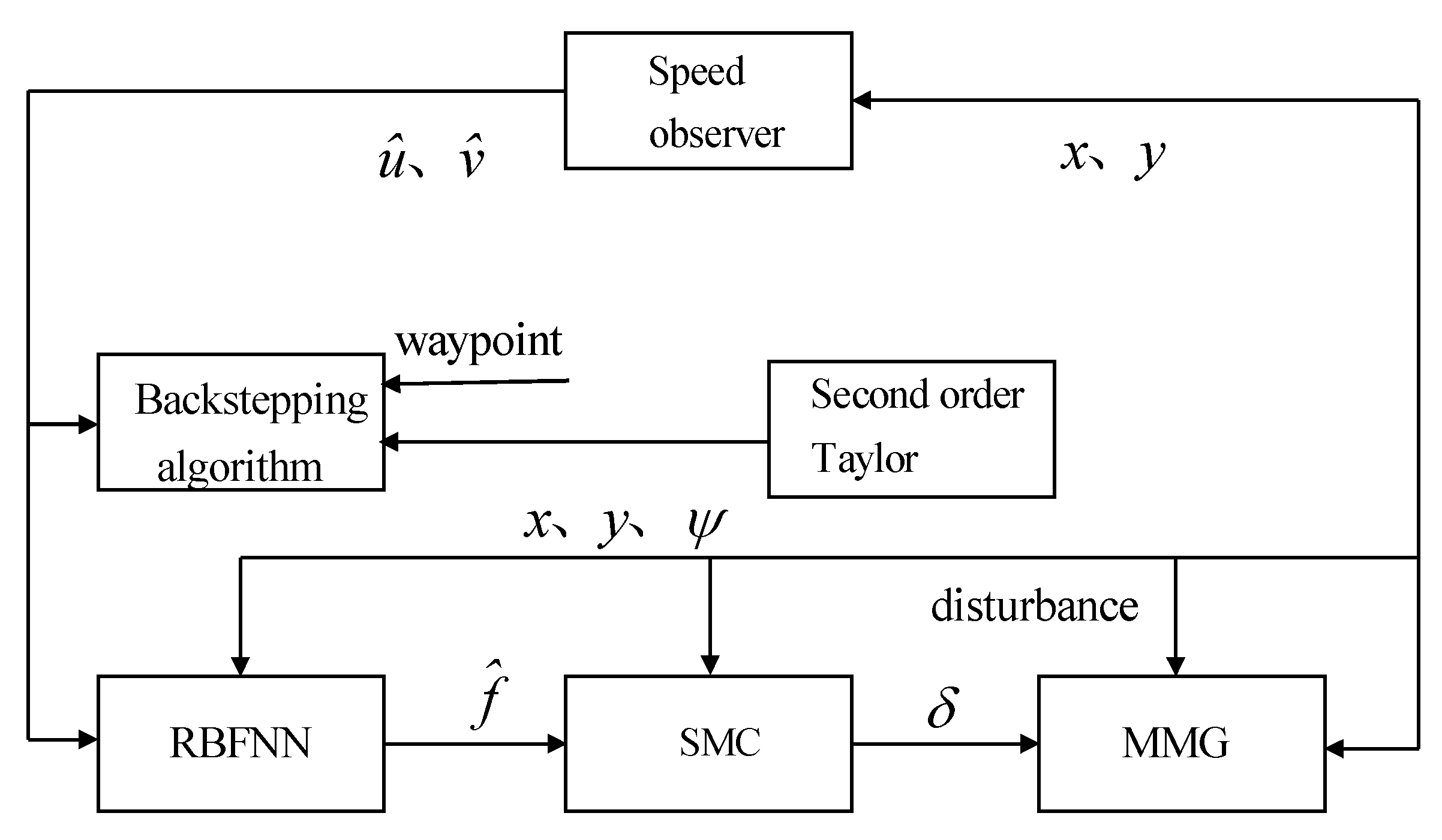
Three-degree-of-freedom track tracking control is transformed into course control by the backstepping algorithm, and the future position is predicted by the second-order Taylor expansion method. The current error and future total error functions are constructed, and the errors are fed back to backstepping to form the desired heading angle in order to solve the problem of the inability to track the waypoint without overshoot in the process of following.
(2)
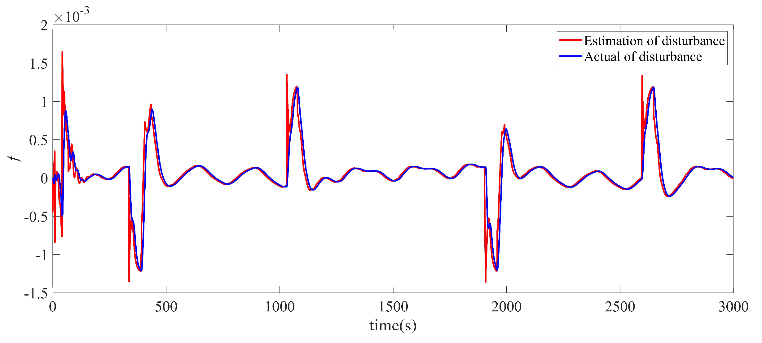
The RBF neural network and sliding mode control are combined to estimate unknown disturbance by the RBF neural network and feedback to the sliding mode controller to solve the external interference and the internal model uncertainty.
(3)
The nonlinear observer is used to obtain the velocity and solve the problem of unknown ship velocity.
The paper is constructed as follows: Firstly, Section 2 introduces the mathematical model of ship motion, including the simulation model and design model. Next, Section 3 describes the design process of the ship motion controller, including backstepping, the RBF neural network, and second-order Taylor formula. Then, Section 4 presents numerical simulation results. The ship path following effect based on position prediction is compared with that without prediction, and the algorithm proposed in this paper is compared with other algorithms. Finally, Section 5 provides the conclusions of this paper.

2. Ship Motion Model

2.1. Simulation Model

With the development of autonomous ship technology, the modeling technique for ship maneuvering motion has attracted wide attention. A reliable mathematical model has a highly practical value for providing accurate motion predictions or designing a control system [30]. In this paper, MMG (the mathematical model group) [31] is used as the mathematical model of ship motion. The MMG model is based on profound theoretical analysis and a large number of experiments. It decomposes the hydrodynamic force (moment) acting on the ship into the hydrodynamic force (moment) acting on the ship, propeller, and rudder, and considers the interaction between the hydrodynamic forces (moments). Figure 1 shows coordinate systems used to describe ship motion. In a world coordinate system, x 0 axis points toward north and y 0 axis points towards east. Here, ( x , y ) is the position of the ship in the world coordinate system. The angle between the center line of the ship’s head and tail and the x0 axis is a course angle called ψ . In a local coordinate system ( u , v ) that is fixed to the ship, u and v axis point toward a surge direction of the ship and a sway direction of the ship, respectively. u and v are the surge velocity and the sway velocity in the local coordinate system. r is the yaw rate of the ship. Total velocity relative to the ground is V = ( u 2 + v 2 ) 1 / 2 , drift angle b = arctan ( v / u ) . δ is the rudder angle.
{ x ˙ = u r cos ψ v r sin ψ + V c cos ψ c = u cos ψ v sin ψ y ˙ = u r sin ψ + v r cos ψ + V c sin ψ c = u sin ψ + v cos ψ ψ ˙ = r u ˙ = [ ( m + m y ) v r + X H + X P + X W + X W A V E + ( m x m y ) V c sin ( ψ c ψ ) r ] / ( m + m x ) v ˙ = [ ( m + m x ) u r + Y H + Y P + Y W + Y W A V E + ( m x m y ) V c cos ( ψ c ψ ) r ] / ( m + m y ) r ˙ = ( N H + N P + N R + N W + N W A V E ) / ( I Z Z + J Z Z )
In Equation (1), m is the mass of the ship; m x and m y are added mass; X H , Y H , and N H are the hydrodynamic forces and moments on the naked hull; X P , Y P , and N P are propeller force (moment); ψ c and V c are flow direction and velocity, respectively, X W , Y W , and NW are wind force (moment); X w a v e , Y w a v e , and N w a v e are wave force (moment); I z z is the moment of inertia of the ship around the vertical axis; J z z is additional moment of inertia; and X R , Y R , and N R are rudder forces (moment), which are calculated as follows:
{ X R = ( 1 t R ) F N sin δ Y R = ( 1 + a H ) F N cos δ N R = ( x R + a H x H ) F N cos δ
In Equation (2), t R is the reduction in rudder resistance, a H is the ratio of additional lateral force caused by the rudder and rudder lateral force, x H is the distance from the center of action of lateral force induced by the rudder to the center of gravity of ship, and F N is the positive pressure of the rudder.

2.2. Design Model

Path following does not need to consider the time factor, so in this paper, the propeller speed is set as a fixed value, only considering the rudder angle input. Therefore, Equation (1) can be simplified as the design model of Equation (3) [17].
{ x ˙ = u cos ψ v sin ψ = u 2 + v 2 cos ( ψ + β ) y ˙ = u sin ψ + v cos ψ = u 2 + v 2 sin ( ψ + β ) ψ ˙ = r r ˙ = r T + K T δ + f β = arctan ( v / u ) f = f 1 + d
In Equation (3), K is the ship’s cyclicity index; T is the following index; f 1 is the internal model uncertainty; d is the external interference uncertainty; and f is the sum of the model uncertainty f 1 and external interference d , that is, the total unknown term. It is difficult to measure the surge velocity u and sway velocity v in practice.

2.3. Wind and Wave Interference Model

In order to verify the effectiveness of the controller below, this section introduces the simulation ship Yulong ship used in this paper. The MMG model in Equation (1) is taken as the simulation model. The parameters of Yulong wheel are the same as [32].
The wind force (moment) X w , Y w and N w in Equation (1) are calculated as follows [33]:
{ X w = 1 2 ρ a A f U R 2 C w x ( α R ) Y w = 1 2 ρ a A s U R 2 C w y ( α R ) N w = 1 2 ρ a A s L o a U R 2 C w n ( α R )
where ρ a is the air density; α R is the relative wind direction angle; U R is the relative wind speed; A f and A s are the forward projection area and side projection area above the waterline of the ship; L o a is the total length of the ship; and C X w ( λ ), C Y w ( λ ), and C N w ( λ ) are the wind pressure (moment) coefficients.
Since large ships can resist the first-order wave interference in their navigation, this paper only considers the second-order wave interference, and the wave forces (moments) X w a v e , Y w a v e , and N w a v e are calculated as follows [34]:
{ X w a v e = 1 2 ρ L α 2 cos χ C X w ( λ ) Y w a v e = 1 2 ρ L α 2 sin χ C Y w ( λ ) N w a v e = 1 2 ρ L α 2 sin χ C N w ( λ )
In Equation (5), λ is wave wavelength; χ is wave encounter angle; ρ is sea water density; α is wave amplitude; L is ship length; and C X w ( λ ), C Y w ( λ ), and C N w ( λ ) are wave drift force (moment) coefficients.

2.4. Assumptions

Since the longitudinal displacement is not considered in the path following, the ship can follow the path by stabilizing the lateral displacement y to 0. Therefore, the control objective of this paper is to set the propeller speed in advance and design the appropriate rudder angle so that the ship can track the reference path, that is, the lateral displacement deviation ye = 0. In the process of designing the controller, the following assumptions are required:
(1)
The ship state values, x , y , and ψ can be obtained.
(2)
The uncertainty f is bounded, that is | f | < f m a x .
(3)
The second derivative of displacements x and y is bounded, i.e., | x ¨ |≤ x ¨ m a x , | y ¨ | < y ¨ m a x .
(4)
The motion of the ship in roll, pitch, and heave directions was neglected.
(5)
The ship had neutral buoyancy, and the origin of the body-fixed coordinate was located at the center of mass [35].

3. Path following Controller

In this paper, the path following controller consists of two parts. The first part is designing the desired heading angle based on the predicted future error and backstepping algorithm; the second part is using the nonlinear sliding mode controller and RBF neural network to realize the course control. The control structure is shown in Figure 2.

3.1. Backstepping Algorithm

This section uses the backstepping algorithm designing the desired heading angle according to the predicted future error. Firstly, the derivation of the lateral displacement deviation y ˙ e = y ˙ y ˙ d is obtained, and Equation (3) is substituted by:
y ˙ e = y ˙ y ˙ d = u 2 + v 2 sin ( ψ + β ) d y d d x d x d t = u 2 + v 2 sin ( ψ + β ) tan θ x ˙ = u 2 + v 2 sin ( ψ + β ) sin θ cos θ u 2 + v 2 cos ( ψ + β ) = cos θ u 2 + v 2 sin ( ψ + β ) sin θ u 2 + v 2 cos ( ψ + β ) = u 2 + v 2 s i n ( ψ + β θ )
According to Equation (6), the desired heading angle is designed as follows:
ψ d = c 0 tanh ( c 1 y e ) β + θ
In Equation (7), c 0 and c 1 are positive design parameters, the Lyapunov function V ˙ 1 = ( 1 / 2 ) y e 2 is selected, and its derivative is obtained:
V ˙ 1 = y e y ˙ e = y e u 2 + v 2 sin ( ( c 0 tanh ( c 1 y e ) β + θ ) + β ) = y e u 2 + v 2 sin ( c 0 tanh ( c 1 y e ) )
Because the value of c0tanh ( c 1 y e ) is between ( π/3, π/3), sin ( c 0 tanh ( c 1 y e ) is an odd function, and the sign is the same as y e . It can be obtained by y e u 2 + v 2 sin ( c 0 tanh ( c 1 y e ) ) ≤ 0; thus, V ˙ ≤ 0. Therefore, the designed reference course Equation (7) can make the path deviation y e tend to 0.
However, in most studies, only the path deviation ye at the current time is considered, which can easily generate overshoot at the turning point. In view of this, this paper predicts the ship’s future position and then considers the path deviation in the present and future time domains. This allows the ship to predict the path ahead of time, thus turning as early as possible to avoid overshooting. First, according to Equation (3) and second-order Taylor expansion, all ship positions in the future time domain n are predicted:
{ y ¯ ( k + 1 ) = y ( k ) + j = 0 0 ( T y ˙ ( k + j ) ) + 1 2 j = 0 0 ( T 2 y ¨ ( k + j ) ) y ¯ ( k + 2 ) = y ( k ) + j = 0 1 ( T y ˙ ( k + j ) ) + 1 2 j = 0 1 ( T 2 y ¨ ( k + j ) ) y ¯ ( k + n ) = y ( k ) + j = 0 n 1 ( T y ˙ ( k + j ) ) + 1 2 j = 0 n 1 ( T 2 y ¨ ( k + j ) )
In Equation (9), y ¯ ( k + n ) is the predicted value of y at k + n , T is the predicted sampling time, and y ˙ ( k + j ) is the discretization result of the second term in Equation (3).
y ˙ ( k + j ) = u ( k ) sin ψ ( k ) + v ( k ) cos ψ ( k )
The future error y ˙ ( k + j ) , j = 1 , 2 , ... n is calculated by the predicted value of Equation (9) and reference path yd; n is as follows:
{ e ¯ y ( k + 1 ) = y ¯ ( k + 1 ) y d ( k + 1 ) e ¯ y ( k + 2 ) = y ¯ ( k + 2 ) y d ( k + 2 ) e ¯ y ( k + n ) = y ¯ ( k + n ) y d ( k + n )
According to Equation (11), the total path error including current time and future time is constructed as follows:
y E ( y , y d ) = P e ¯ y ( k ) + j = 1 n Q e ¯ y ( k + j )
In Equation (12), P and Q are weights to adjust the balance between current time error and future error.
According to Equation (12), the virtual reference course is designed as follows:
ψ d = c 1 tanh ( c 0 y E ) β + θ

3.2. Design of RBF Neural Network Controller

The RBF neural network can approximate any nonlinear function, deal with the laws that are difficult to analyze in the system, has a good generalization ability, and has a fast learning convergence speed [24]. In the RBF network, x = ( x i ) T is the input of the network, the output of the hidden layer of the network is h = ( h j ) T , and h j is the output of the j neuron of the hidden layer
h j = e x p ( x c i j 2 2 b j 2 )
In Equation (14), c i j is the coordinate vector of the center point of the Gaussian basis function of the j neuron in the hidden layer, and b j is the width of the Gaussian basis function of the j neuron in the hidden layer. The network weight of the RBF is w , and the output of the RBF network is y ( t ) = w T h .
The second-order ship motion system is a nonlinear system. δ and y are the input and output of the system, respectively. f is the external disturbance and the total disturbance of the system. The desired heading angle of the ship is calculated by the backstepping method. According to the error, nonlinear sliding surface are designed as
s = ψ ˙ e + c 2 tanh ( c 3 ψ e )
In Equation (15), c 2 and c 3 are positive design parameters. The derivation of Equation (15) is correct
{ s ˙ = ψ ¨ e + a ˙ a = c 2 tanh ( c 3 ψ e )
By substituting Equation (1) into Equation (16)
s ˙ = 1 T r + K T δ + f ψ ¨ d + a ˙
In order to make the sliding surface s tend to be stable, let
s ˙ = c 4 s
Equation (18) c 4 is a positive design parameter. Then, the sliding mode control law is designed as follows:
δ = T K ( c 4 s + ψ ¨ d + r T f a ˙ )
Since f is an unknown term, it is approximated by the RBF, so the RBF neural network is used to approximate f , where
f = W * T h ( x ) + e
where W * is the ideal weight of the network, ε is the approximation error of the network, and | e | e M and f are the output of the ideal RBF network. If the input of the network is defined as ψ e , the output of the RBF is
f ^ = W ^ T h ( x )
where f ^ is the estimated value of f . Then, Equation (19) can be written as
δ = T K ( c 4 s + ψ ¨ d + r T f ^ a ˙ )
By substituting Equation (22) into Equation (17),
f ˜ = f ^ f = W ^ T h ( x ) W * T h ( x ) e = W ˜ T h ( x ) e
s ˙ = W ˜ T h ( x ) e c 4 s
In Equation (23), f ˜ is the estimation error of the unknown term f and W ^ is the estimation weight. The Lyapunov function is selected as follows:
V 2 = 1 2 s 2 + 1 2 ξ ( W ^ W ) 2
In Equation (25), ξ is a positive coefficient and the derivative of V2 is as follows:
V ˙ 2 = s s ˙ + ξ ( W ^ W ) W ^ ˙ = s ( c 4 s + f f ^ ) + ξ ( W ^ W ) W ^ ˙ = c 4 s 2 + ( W ^ W ) ( s h ( x ) ξ W ^ ˙ ) + e s
Let W ^ ˙ = s h ( x ) / ξ ; then, V ˙ 2 = c 4 s 2 + e s , because e is the approximation error of the network, which can be limited enough in theory, so
V ˙ 2 = c 4 s 2 + e s 0
Thus, the proofs of RBF sliding mode control were investigated.

3.3. Nonlinear Velocity Observer

In this section, a nonlinear velocity observer is used to estimate surge velocity u and sway velocity v . First, the derivatives of displacement x ˙ and y ˙ are estimated:
{ x ^ ˙ = x ˙ ^ k x 1 ( x ^ x ) x ˙ ^ ˙ = k x 2 tanh ( x ^ x ) y ^ ˙ = y ˙ ^ k y 1 ( y ^ y ) y ˙ ^ ˙ = k y 2 tanh ( y ^ y )
In Equation (28) x ^ , x ˙ ^ , y ^ , and y ˙ ^ represent x , x ˙ , y , and y ˙ , respectively, while k x 1 , k x 2 , k y 1 , and k y 2 are the design parameters. Taking x as an example, the Lyapunov function is selected:
V 3 = 1 2 γ ( x ^ x ) 2 + 1 2 ( x ˙ ^ x ˙ ) 2
In Equation (29), γ is a positive coefficient, and the derivation of Equation (29) is as follows:
{ V ˙ 3 = γ ( x ^ x ) ( x ^ ˙ x ˙ ) + ( x ˙ ^ x ˙ ) ( x ˙ ^ ˙ x ¨ ) = γ ( x ^ x ) ( x ˙ ^ k x 1 ( x ^ x ) x ˙ ) + ( x ˙ ^ x ˙ ) ( k x 2 tanh ( x ^ x ) x ¨ ) = γ k x 1 ( x ^ x ) 2 z 1 z 2 z 3 z 1 = x ˙ ^ x ˙ z 2 = k x 2 tanh ( x ^ x ) γ k x 1 ( x ^ x ) z 3 = x ¨ ( x ˙ ^ x ˙ )
According to assumption (3), z 3 is negligible. Since the hyperbolic tangent function is strictly bounded, choosing the appropriate positive parameter k x 1 > k x 2 can make z 2 and the different sign; that is, when z 2 is greater than 0, at this time, the second term in Equation (30) will be greater than 0, and then it will be increased, meaning that z 1 and z 2 will be greater than zero. Similarly, if z 2 is less than 0, the second term in Equation (30) will also be less than 0, and, thus, it will be reduced so that z 1 and z 2 will both be less than zero and will still be a problem. The proof process of y is the same, so it is not described here. According to the estimated values of x ˙ and y ˙ , the kinematic equation in Equation (3) is transformed:
{ u ^ = y ˙ ^ sin ψ + x ˙ ^ cos ψ v ^ = y ˙ ^ cos ψ x ˙ ^ sin ψ

4. Simulation Results

4.1. Comparative Experiment for Position Prediction

In this section, the position prediction strategy is compared with the without-position prediction strategy, and some interesting conclusions can be obtained. The following waypoints are shown in Table 1, and the simulation results are shown in Figure 3 and Figure 4.
In Figure 3, the red line indicates that there is no path following effect based on position prediction, the blue line is the tracking effect based on position prediction, and the black line is the reference path. For the quantified analysis, the important performance index ‘overshoot’ is presented to verify the conclusion. When the path following has no predicted position, the prediction range is n = 0, and the overshoot of path following is 97.1 m. When the path following has a predicted position, the prediction range is n = 45. Considering the future path and deviation, the steering point can be steered in advance, so the path following has basically no overshoot.
In Figure 4, the red line indicates the value of path following error without position prediction, and the blue line indicates the value of path following error based on position prediction. It can be seen from the figure that the initial error of path following is 300 m. Under the action of the controller, the error begins to decrease slowly, and the path following based on prediction has a better effect. There is basically no overshoot compared with no prediction.

4.2. Comparative Experiment for Control Algorithm

To verify the performance of the proposed control algorithm, a comparison with the method used in [32] is given in this section. The ship initial states are shown in Table 2. External interference: wind speed: 10 m/s; wind direction: 30sin (0.02t) + 45; velocity: 1.0 m/s; flow direction: 10sin (0.005t) + 45; wave wavelength: 83 m; wave encounter angle: 135°–30°sin(0.02t). The controller parameters are c 0 = 0.003, c 1 = π/3, c 2 = 0.1, c 3 = 0.4, and c 4 = 0.1; the speed observer parameters are k x 1 = 0.58, k x 2 = 0.15, k y 1 = 0.55, and k y 2 = 0.1; the parameters of Gaussian function are (−5 −2.5 0 2.5 5), b j = 0.25.For more details about the parameter setting of the compared algorithm, the readers are suggested to refer to [32].
The final comparative results are presented in Figure 5, Figure 6 and Figure 7. Figure 5 shows the path following effect of different algorithms. It is noted that both schemes could achieve the effective path following for the designed reference path. Moreover, through attentive observation, it is obvious that the proposed algorithm in this paper has a better follow effect than that of the algorithm proposed in [32]. Figure 6 shows the course changes of the two algorithms in the process of ship motion. Due to the influence of time-varying wind, wave, and current interference, there are small amplitude oscillations in the course to resist the external effect of disturbance. Figure 7 shows the curve of the rudder angle changing with time. Similarly, due to the influence of time-varying wind, wave, and current interference, the rudder angle oscillates slightly. However, careful observation shows that the average rudder angle of the algorithm proposed in this paper is significantly reduced compared with the algorithm in [32]. Because the high steering frequency will cause the crew discomfort and reduce the stability of the ship during navigation, the algorithm proposed in this paper has better navigation practicality.
For the quantitative purpose, some popular performance indexes (Equation (32)) are utilized to evaluate the comparison result [18], e.g., the mean absolute error (MAE) and the mean absolute control effort (MAC). MAE reveals the stabilizing performance of the control system. MAC indicates energy consumption. The specific data are shown in Table 3. It can be observed that the proposed control algorithm has more advantages in many aspects.
MAE = 1 t f t 0 t 0 t f | y e | dt MAC = 1 t f t 0 t 0 t f | δ r | dt

4.3. Verification of Effectiveness of Neural Network and Velocity Observer

Figure 8, Figure 9 and Figure 10 show the observation effect of the speed observer and the estimation effect of the RBF neural network.
Figure 8 describes the observation ability of the designed nonlinear observer for longitudinal velocity u and transverse velocity v . It is obvious that the designed observer can accurately estimate u and v . Figure 9 shows the observation error of the speed observer. Because the initial speed of the ship is not zero and the wind and wave disturbance sometimes changes, the velocity observer has a large error at the beginning. With the increase in time, the error tends to zero, and the error of the observer is not more than 0.2 m/s, showing the effectiveness of the speed observer. Figure 10 shows the approximation ability of the introduced RBF neural network in regard to the total unknown term. The results show that the designed RBF neural network can approach f effectively.

5. Conclusions

In order to solve the problems of velocity measurement, uncertain model, and external interference in the under-drive ship path following, a sliding mode control algorithm is used based on position prediction with the radial basis function. Firstly, in order to make the ship turn ahead of time at the turning point, the ship position is predicted. Based on the predicted value and the reference path value, the future error of the path is calculated in advance, and the reference heading angle is designed by a backstepping algorithm. Secondly, the hyperbolic tangent function is used to design the sliding surface, and the course is controlled by sliding mode control. In order to improve the robustness of the controller, an RBF neural network is introduced to approach the external interference and uncertain parameters. The u and v are estimated by using nonlinear observers to avoid the problem of a velocity difficult to obtain. The simulation results show that the controller can keep the ship accurately tracking the reference path under wind and wave disturbance and turn the rudder in advance at the turning point to avoid overshoot. These results verify the effectiveness of the proposed control algorithm. Because the computer simulation is only used in this paper, and no real ship simulation is adopted, our next study will consider the problem of ship path following in the case of a real ship.

Author Contributions

Conceptualization, H.Z.; methodology, H.Z.; software, H.Z.; validation, H.Z.; formal analysis, H.Z.; writing—original draft preparation, H.Z.; writing—review and editing, X.Z. and R.B.; visualization, H.Z.; supervision, X.Z. and R.B.; funding acquisition, X.Z. All authors have read and agreed to the published version of the manuscript.

Funding

This research was funded by the National Science Foundation of China, grant number 51679024.

Institutional Review Board Statement

Not applicable.

Informed Consent Statement

Not applicable.

Data Availability Statement

The data that support the findings of this study are available from the corresponding author upon reasonable request.

Acknowledgments

Much appreciation to each reviewer for their valuable comments and suggestions to improve the quality of this note. This work is partially supported by the National Science Foundation of China (Grant No.51679024) The authors would like to thank anonymous reviewers for their valuable comments to improve the quality of this article.

Conflicts of Interest

The authors declare no conflict of interest.

References

  1. Nagai, T.; Watanabe, R. Applying Position Prediction Model for Path Following of Ship on Curved Path. In Proceedings of the 2016 IEEE Region 10 Conference (TENCON), Singapore, 22–25 November 2016; pp. 3675–3678. [Google Scholar]
  2. Hu, X.; Wei, X.; Zhu, G.; Wu, D. Adaptive synchronization for surface vessels with disturbances and saturated thruster dynamics. Ocean Eng. 2020, 216, 107920. [Google Scholar] [CrossRef]
  3. Hu, X.; Wei, X.; Han, J.; Zhu, X. Adaptive Disturbance Estimation and Cancelation for Ships under Thruster Saturation. Int. J. Robust Nonlinear Control. 2020, 30, 5004–5020. [Google Scholar] [CrossRef]
  4. Zhang, H.; Zhang, X.; Bu, R. Active Disturbance Rejection Control of Ship Course Keeping Based on Nonlinear Feedback and ZOH Component. Ocean Eng. 2021, 233, 109136. [Google Scholar] [CrossRef]
  5. Vu, M.T.; Le Thanh, H.N.N.; Huynh, T.-T.; Thang, Q.; Duc, T.; Hoang, Q.-D.; Le, T.-H. Station-Keeping Control of a Hovering Over-Actuated Autonomous Underwater Vehicle Under Ocean Current Effects and Model Uncertainties in Horizontal Plane. IEEE Access 2021, 9, 6855–6867. [Google Scholar] [CrossRef]
  6. Vu, M.T.; Le, T.-H.; Thanh, H.L.N.N.; Huynh, T.-T.; Van, M.; Hoang, Q.-D.; Do, T.D. Robust Position Control of an Over-Actuated Underwater Vehicle under Model Uncertainties and Ocean Current Effects Using Dynamic Sliding Mode Surface and Optimal Allocation Control. Sensors 2021, 21, 747. [Google Scholar] [CrossRef]
  7. Zhang, G.; Zhang, X. Concise Robust Adaptive Path-Following Control of Underactuated Ships Using DSC and MLP. IEEE J. Ocean. Eng. 2014, 39, 685–694. [Google Scholar] [CrossRef]
  8. Peng, Z.; Wang, J.; Han, Q.-L. Path-Following Control of Autonomous Underwater Vehicles Subject to Velocity and Input Constraints via Neurodynamic Optimization. IEEE Trans. Ind. Electron. 2019, 66, 8724–8732. [Google Scholar] [CrossRef]
  9. Deng, Y. Model-Based Event-Triggered Tracking Control of Underactuated Surface Vessels With Minimum Learning Parameters. IEEE Trans. Neural Netw. Learn. Syst. 2020, 31, 14. [Google Scholar] [CrossRef]
  10. Liu, C.; Negenborn, R.R.; Chu, X.; Zheng, H. Predictive Path Following Based on Adaptive Line-of-Sight for Underactuated Autonomous Surface Vessels. J. Mar. Sci. Technol. 2018, 23, 483–494. [Google Scholar] [CrossRef]
  11. Liu, L.; Wang, D.; Peng, Z.; Wang, H. Predictor-Based LOS Guidance Law for Path Following of Underactuated Marine Surface Vehicles with Sideslip Compensation. Ocean Eng. 2016, 124, 340–348. [Google Scholar] [CrossRef]
  12. Xu, H.; Fossen, T.I.; Guedes Soares, C. Uniformly Semiglobally Exponential Stability of Vector Field Guidance Law and Autopilot for Path-Following. Eur. J. Control 2020, 53, 88–97. [Google Scholar] [CrossRef]
  13. Perera, L.P.; Guedes Soares, C. Pre-Filtered Sliding Mode Control for Nonlinear Ship Steering Associated with Disturbances. Ocean Eng. 2012, 51, 49–62. [Google Scholar] [CrossRef]
  14. Fossen, T.I.; Breivik, M.; Skjetne, R. Line-of-Sight Path Following of Underactuated Marine Craft. IFAC Proc. Vol. 2003, 36, 211–216. [Google Scholar] [CrossRef]
  15. Lekkas, A.M.; Fossen, T.I. Integral LOS Path Following for Curved Paths Based on a Monotone Cubic Hermite Spline Parametrization. IEEE Trans. Contr. Syst. Technol. 2014, 22, 2287–2301. [Google Scholar] [CrossRef]
  16. Moreira, L.; Fossen, T.I.; Guedes Soares, C. Path Following Control System for a Tanker Ship Model. Ocean Eng. 2007, 34, 2074–2085. [Google Scholar] [CrossRef]
  17. Li, Z.; Li, R.; Bu, R. Path Following of Under-Actuated Ships Based on Model Predictive Control with State Observer. J. Mar. Sci. Technol. 2021, 26, 408–418. [Google Scholar] [CrossRef]
  18. Deng, Y.; Zhang, X.; Zhang, G. Line-of-Sight-Based Guidance and Adaptive Neural Path-Following Control for Sailboats. IEEE J. Ocean. Eng. 2020, 45, 1177–1189. [Google Scholar] [CrossRef]
  19. Kelasidi, E.; Liljeback, P.; Pettersen, K.Y.; Gravdahl, J.T. Integral Line-of-Sight Guidance for Path Following Control of Underwater Snake Robots: Theory and Experiments. IEEE Trans. Robot. 2017, 33, 610–628. [Google Scholar] [CrossRef] [Green Version]
  20. Qu, Y.; Xiao, B.; Fu, Z.; Yuan, D. Trajectory Exponential Tracking Control of Unmanned Surface Ships with External Disturbance and System Uncertainties. ISA Trans. 2018, 78, 47–55. [Google Scholar] [CrossRef] [PubMed]
  21. Borkowski, P.; Zwierzewicz, Z. Ship Course-Keeping Algorithm Based On Knowledge Base. Intell. Autom. Soft Comput. 2011, 17, 149–163. [Google Scholar] [CrossRef]
  22. Weng, Y.; Wang, N.; Guedes Soares, C. Data-Driven Sideslip Observer-Based Adaptive Sliding-Mode Path-Following Control of Underactuated Marine Vessels. Ocean Eng. 2020, 197, 106910. [Google Scholar] [CrossRef]
  23. Moreira, L.; Guedes Soares, C. Dynamic Model of Manoeuvrability Using Recursive Neural Networks. Ocean Eng. 2003, 30, 1669–1697. [Google Scholar] [CrossRef]
  24. Li, R.; Huang, J.; Pan, X.; Hu, Q.; Huang, Z. Path Following of Underactuated Surface Ships Based on Model Predictive Control with Neural Network. Int. J. Adv. Robot. Syst. 2020, 17. [Google Scholar] [CrossRef]
  25. Wang, D.; Huang, J. Neural Network Based Adaptive Dynamic Surface Control for Nonlinear Systems in Strict-Feedback Form. In Proceedings of the 40th IEEE Conference on Decision and Control (Cat. No.01CH37228), Orlando, FL, USA, 4–7 December 2001; pp. 3524–3529. [Google Scholar]
  26. Yu, Z.; Zhang, Y.; Liu, Z.; Qu, Y.; Su, C.-Y.; Jiang, B. Decentralized Finite-Time Adaptive Fault-Tolerant Synchronization Tracking Control for Multiple UAVs with Prescribed Performance. J. Frankl. Inst. 2020, 357, 11830–11862. [Google Scholar] [CrossRef]
  27. Yin, J.-C.; Perakis, A.N.; Wang, N. A Real-Time Ship Roll Motion Prediction Using Wavelet Transform and Variable RBF Network. Ocean Eng. 2018, 160, 10–19. [Google Scholar] [CrossRef]
  28. Zhang, G.; Zhang, C.; Li, J.; Zhang, X. Improved Composite Learning Path-Following Control for the Underactuated Cable-Laying Ship via the Double Layers Logical Guidance. Ocean Eng. 2020, 207, 107342. [Google Scholar] [CrossRef]
  29. Yin, J.; Zou, Z.; Xu, F. On-Line Prediction of Ship Roll Motion during Maneuvering Using Sequential Learning RBF Neural Networks. Ocean Eng. 2013, 61, 139–147. [Google Scholar] [CrossRef]
  30. Wang, Z.; Xu, H.; Xia, L.; Zou, Z.; Soares, C.G. Kernel-Based Support Vector Regression for Nonparametric Modeling of Ship Maneuvering Motion. Ocean Eng. 2020, 216, 107994. [Google Scholar] [CrossRef]
  31. Zhang, W.; Zou, Z.-J.; Deng, D.-H. A Study on Prediction of Ship Maneuvering in Regular Waves. Ocean Eng. 2017, 137, 367–381. [Google Scholar] [CrossRef]
  32. Li, R.; Jia, B.; Fan, S.; Pan, X. A Novel Active Disturbance Rejection Control with Hyperbolic Tangent Function for Path Following of Underactuated Marine Surface Ships. Meas. Control 2020, 53, 1579–1588. [Google Scholar] [CrossRef]
  33. Wang, J.; Zou, Z.; Wang, T. Path Following of a Ship Sailing in Restricted Waters Based on an Extended Updated-Gain High-Gain Observer. In Proceedings of the International Conference on Offshore Mechanics and Arctic Engineering, Madrid, Spain, 17 June 2018; p. V07BT06A030. [Google Scholar]
  34. Xiaobin, Q.; Yong, Y.; Helong, S.; Xiaofeng, S.; Xiufeng, Z. Simulation System for Testing Ship Dynamic Positioning Control Algorithm. J. Syst. Simul. 2016, 28, 2028–2034. [Google Scholar]
  35. Vu, M.T.; Van, M.; Bui, D.H.P.; Do, Q.T.; Huynh, T.-T.; Lee, S.-D.; Choi, H.-S. Study on Dynamic Behavior of Unmanned Surface Vehicle-Linked Unmanned Underwater Vehicle System for Underwater Exploration. Sensors 2020, 20, 1329. [Google Scholar] [CrossRef] [PubMed] [Green Version]
Figure 1. Ship plane position and motion parameters.
Jmse 09 01055 g001
Figure 2. Whole control structure.
Jmse 09 01055 g002
Figure 3. Simulation comparison of ship path following with and without position prediction.
Jmse 09 01055 g003
Figure 4. Simulation comparison of ship path following with and without position prediction.
Jmse 09 01055 g004
Figure 5. Comparison of path following: proposed algorithm and control method in [32].
Jmse 09 01055 g005
Figure 6. Comparison of course angle: proposed algorithm and control method in [32].
Jmse 09 01055 g006
Figure 7. Comparison of rudder angle: proposed algorithm and control method in [32].
Jmse 09 01055 g007
Figure 8. Comparison of estimated velocity and actual velocity.
Jmse 09 01055 g008
Figure 9. Error duration curve of estimated velocity and actual velocity.
Jmse 09 01055 g009
Figure 10. Estimation of disturbance and actual disturbance.
Jmse 09 01055 g010
Table 1. Ship reference waypoint.
Desired WaypointCoordinate
Waypoint 1(0,0)
Waypoint 2(2000,0)
Waypoint 3(4000,2000)
Waypoint 4(8000,2000)
Waypoint 5(10,000,4000)
Table 2. Ship initial parameters.
Ship Initial StatesValue
surge velocity u7.2 m/s
sway velocity v0 m/s
yaw rate r0 m/s
course
position coordinate (x,y)(0,300)
Table 3. Quantitative performance comparison of both algorithms.
Algorithm TypesMAEMAC
The proposed algorithm3.82 m8.12 deg
The algorithm in [32]5.12 m9.07 deg
Publisher’s Note: MDPI stays neutral with regard to jurisdictional claims in published maps and institutional affiliations.

