Article

RANS Computation of the Mean Forces and Moments, and Wave-Induced Six Degrees of Freedom Motions for a Ship Moving Obliquely in Regular Head and Beam Waves

1
Key Laboratory of High Performance Ship Technology, Wuhan University of Technology, Ministry of Education, Wuhan 430070, China
2
School of Naval Architecture, Ocean and Energy Power Engineering, Wuhan University of Technology, Wuhan 430070, China
*
Authors to whom correspondence should be addressed.
J. Mar. Sci. Eng. 2021, 9(11), 1176; https://doi.org/10.3390/jmse9111176
Submission received: 28 September 2021 / Revised: 19 October 2021 / Accepted: 20 October 2021 / Published: 26 October 2021
(This article belongs to the Special Issue Manoeuvring and Control of Ships and Other Marine Vehicles)

Abstract

:
Ship maneuvering performance in waves has attracted much attention in recent years. One of main research efforts for this problem has been devoted to the high-accuracy computation of hydrodynamic forces and moments, as well as wave-induced motions, for ships performing maneuvering motions in waves. The objective of this article is to present a numerical study on the computation of the mean forces and moments, and wave-induced six degrees of freedom motions for a ship moving obliquely in regular head and beam waves. The RANS (Reynolds-Averaged Navier-Stokes) solver based on OpenFOAM is used for this purpose. The RANS computations herein are carried out in a horizontal coordinate system. The numerical wave maker with prescribing values of flow variables on the domain boundaries is applied for the wave generation in the computational domain. However, in order to prevent wave reflection, relaxed zones adjacent to the wave maker boundaries are set up. A new program module is inserted into OpenFOAM to update the flow velocity and wave evaluation on the wave-maker boundaries and in the relaxed zones during the RANS computation. The mesh deformation method is employed to allow the ship to perform motions in space. However, a virtual spring system is attached to the ship so as to restrain the surge, sway and yaw, while heave, pitch and roll are completely free, so that the ship is able to oscillate periodically around a certain position in space. The computed mean forces and moments with the inertia effects agree fairly well with the experimental data, and the computed wave-induced motions are also in quite reasonable agreement with the experimental data. This study shows a very successful computation, as well as the procedure of the RANS results processing.

1. Introduction

Nowadays, demands for green ships are strongly increasing, in line with the requirements of energy-saving and emission reduction. To this end, we need to use lower-power ship machineries for the reduction of energy consumption. However, ships are bound to encounter severe environments when travelling, which in reverse requires that ships must have sufficient power to overcome the severe environment for safe navigation. Thus, the accurate and efficient evaluation of ship performance in real sea conditions becomes more and more imperative at the initial stage of ship design.
When controlling a ship in waves, the ship trajectory will be affected by wave drift effects, e.g., the ship’s turning circle becomes twisted during a turning motion, compared with that in calm water. Meanwhile, the ship will oscillate in space, mainly due to the first-order wave forces and moments. These phenomena increase the risk of ship getting out of control, or even capsizing in an extreme wave environment.
Unfortunately, the development of an acceptable method of predicting ship maneuverability in waves has remained a great challenge so far. Generally speaking, the challenge may be mainly due to the difficulties in computing the hydrodynamic forces and moments acting on a ship with high accuracy and efficiency, because as long as the forces and moments in ship motion equations are of high accuracy, ship maneuverability can be accurately predicted by solving the motion equations. Carrica et al. [1] solved 6DOF (Six Degrees of Freedom) ship motion equations to predict rudder maneuvers in waves, where the forces and moments in motion equations are computed by RANS (Reynolds-Averaged Navier-Stokes) method. Note that the ship motion equations solved by the authors were transient. To instantly compute the forces and moments by RANS method is still time-consuming at present, especially considering ship 6DOF motions and real rotating propellers. Another method usually used for ship maneuvering prediction in waves is based on system simulation. This kind of method often separates the transient ship motion problem into a coupling problem of maneuvering and seakeeping. The former is a low-frequency ship motion problem, whereas the latter is of high frequency. In order to analyze them separately, it first requires us to clarify the mechanical mechanism of the coupling problem, e.g., to identify and separate the low-frequency and high-frequency forces and moments correctly.
The two time-scale method is very popular now for predicting maneuverability and seakeeping separately, e.g., in the works of Yasukawa [2,3], Skejic and Faltinsen [4], Zhang et al. [5] and Lee et al. [6]. For such a method, maneuvering performance and seakeeping performance are separately predicted by solving a group of low-frequency ship motion equations and a group of high-frequency ship motion equations. Yao et al. [7] recommended the pure low-frequency and pure high-frequency ship motion equations in regular waves. The low-frequency wave forces and moments in the group of low-frequency motion equations, and high-frequency wave forces and moments in the group of high-frequency motion equations, could be computed by means of a numerical method based on PFT (Potential Flow Theory). The PFT-based methods have advantages in computational efficiency. However, it is generally recognized that the maneuvering forces and moments in calm water computed by PFT-based methods are of low accuracy in practice. The accuracy of the ship maneuvering forces and moments in waves computed by PFT-based methods may be questionable as well. High-accuracy computations of wave forces and moments for coupling cases of maneuvering and seakeeping using PFT-based methods have not yet been reported, although many efforts have been devoted to that, e.g., in the works of Yasukawa et al. [8] and Zhang et al. [9].
Although the numerical method based on the solution of RANS equations is time-consuming for the computation of the hydrodynamic forces and moments acting on ships in waves, this kind of method is more accurate in theory. The relevant non-linear hydrodynamics can be dealt with in a more reasonable manner, especially for maneuvering problems. Until now, just a few studies on the computation of the hydrodynamic forces and moments, as well as the motions, for a maneuvering ship in waves by the RANS method have been reported, e.g., the works by Zhu et al. [10] and Uharek [11]. However, RANS accuracy needs to be further investigated. In addition, the way in which to extract the low-frequency and high-frequency components of forces, moments or motions from RANS results is of great interest, as it is quite essential for the development of new modelling approaches to predict ship maneuverability in waves.
In this work, we employ the RANS technique based on OpenFOAM to compute the mean forces and moments and wave-induced 6DOF Motions for the container ship S-175 moving obliquely in regular head and beam waves. The relevant methodologies, including RANS method and the post processing of RANS results, etc., are described. Great efforts are devoted to the implementation of a new boundary condition module into OpenFOAM, by which the values of freestream flow relative to the ship can be specified on the wave boundaries. The other concern is the post processing of RANS results, e.g., the procedure to compute the mean forces and moments with inertia effects. The numerical results are compared with experimental data, and good agreements are observed. This study shows a very successful computation, as well as the procedure of RANS results processing.

2. Methodology

2.1. Description of the Problem

In order to investigate a ship’s hydrodynamic performance in waves by means of a towing tank test, it is generally required to use something like soft rope or a spring to restrict the ship’s slow-drift motions of surge, sway and yaw due to the waves. 
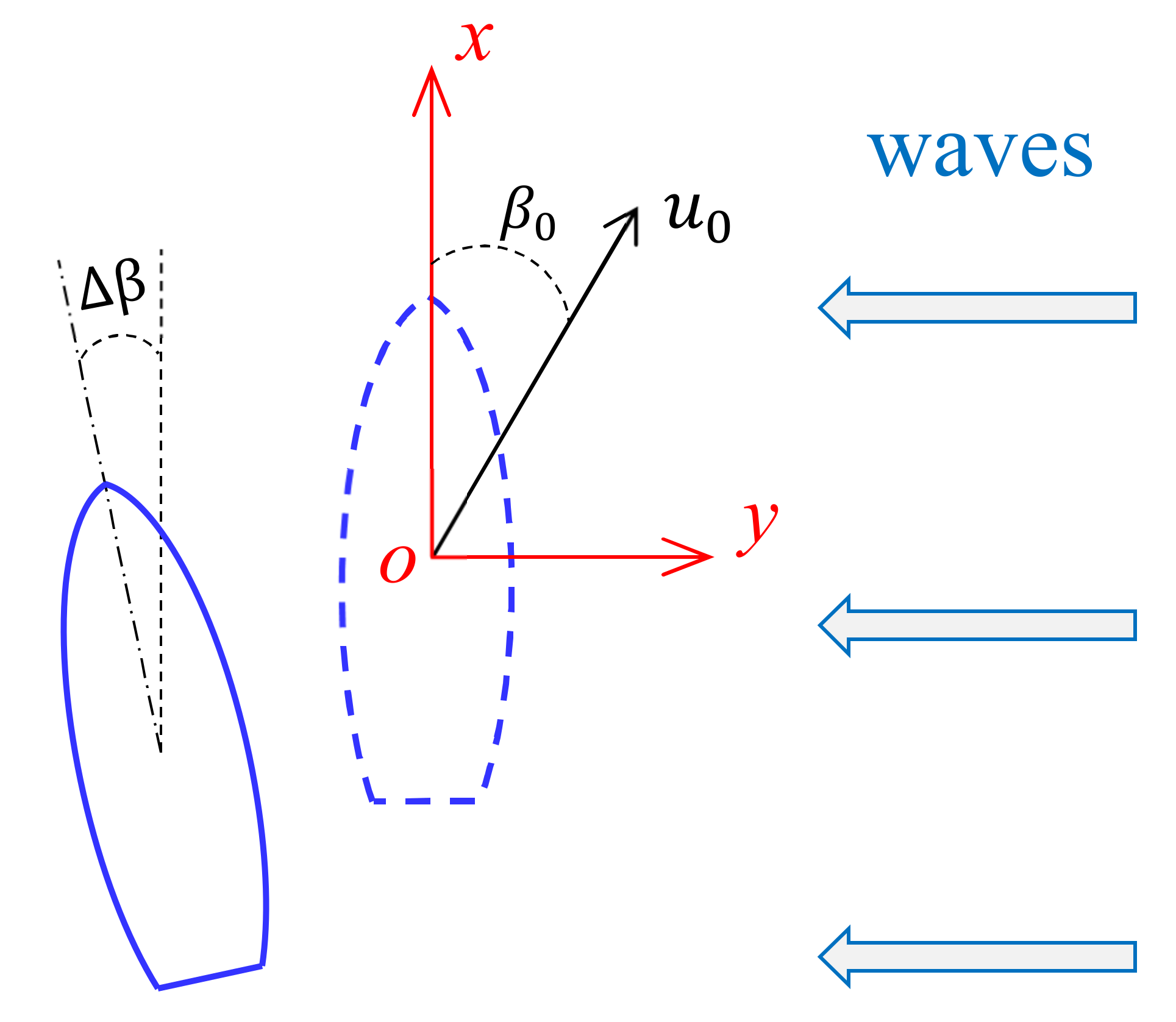
Figure 1 illustrates the situation of a ship model towed obliquely in regular beam waves. The oblique angle β 0 is defined in the horizontal plane when the ship (shown by the dashed line in Figure 1) is towed obliquely with a velocity of u 0 in calm water. Due to the actions of both the waves and spring, the ship will oscillate periodically around a mean position in space. The mean position, e.g., the position of the ship shown by the solid line in Figure 1, is determined by u 0 , β 0 , spring stiffness, wave length, wave height, and wave incident angle. In such a situation, the mean ship heading is different from the ship heading in calm water, and the mean oblique angle can be assumed as β ¯ = β 0 + β , where β is caused by the spring and slow-drift effects of waves. Note that β is not zero when the ship moves obliquely, even in calm water, because the deformation of the spring system will occur, producing forces and moments which balance the hydrodynamic forces and moments acting on the ship. Therefore, the real oblique angle β in calm water is also a sum of β 0 and β . It is the same thing for the wave incident angle. If the wave incident angle χ 0 is defined in the horizontal plane when the ship is at rest in calm water, the real-time incident wave angle χ will change periodically as the ship oscillates in the waves, and the mean incident wave angle χ ¯ is then χ 0 + χ , where χ is caused by the spring and slow-drift effects of waves as well.
For the problem of ship maneuvering in waves, we sometimes prefer to analyze maneuvering and seakeeping separately, although they are coupled in nature. The problem of maneuvering is regarded as a problem of low-frequency ship motion, whereas seakeeping is of high frequency, as mentioned above. It is necessary to separate these two kinds of forces, moments and ship motions, when analyzing them separately. For the situation shown in Figure 1, because the ship oscillates periodically, the transient force or moment acting on the ship, as well as the transient ship motion, may be generally expressed in series form:
ϕ = ϕ 0 + ϕ w + ϕ s ϕ w = n = 1 a n cos n ω e t + b n sin n ω e t ϕ s = m = 1 c m cos m ω s t + d m sin m ω s t
where ϕ represents a general variable of force, moment or ship motion; ω e is wave encounter frequency, which should be understood as the mean encounter frequency; and ω s is natural frequency of the spring. The wave-induced component ϕ w contains the terms with the frequencies n ω e , where n runs from 1 to . The component ϕ s arises from the spring.
For ship maneuvering, the low-frequency forces and moments acting on the ship, as well as low-frequency motions, are usually of more concern. Note that ϕ is a transient variable. If we perform a time average operation to ϕ over an appropriate time interval, the components ϕ w and ϕ s can be completely filtered out, and it then results in ϕ ¯ = ϕ 0 . Obviously, ϕ 0 is a constant of the zeroth order. It may be assumed that the frequency of ϕ 0 is zero or its period is . Thus, ϕ 0 or ϕ ¯ are of low frequency. For seakeeping, the wave-induced high-frequency component ϕ w is more interesting. The interference of the spring is undesirable or even harmful to component analysis, as the components ϕ 0 and ϕ w will be disturbed by the spring, and do not include just the pure effects of the ship maneuvering motions and waves. In order to reduce the interference, ω s must be far from ω e , avoiding resonance. Certainly, the ship maneuvering motions, waves and spring will contribute to the components ϕ 0 , ϕ w and ϕ s .
In this study, we attempt to compute the mean forces and moments, and the wave-induced 6DOF motions for the container ship S-175 moving obliquely in regular head and beam waves by employing the RANS technique based on OpenFOAM, as mentioned. The principal dimensions of S-175 are listed in Table 1. All of the RANS computations are performed for a bare ship model 3.5 m long. The ship towing speed u 0 is 0.879 m/s, corresponding to the Froude number F n = 0.15 and the Reynolds number R e = 3.08 × 10 6 . The oblique angles β 0 considered are 5 ° , 0 ° , 5 ° and 10 ° 
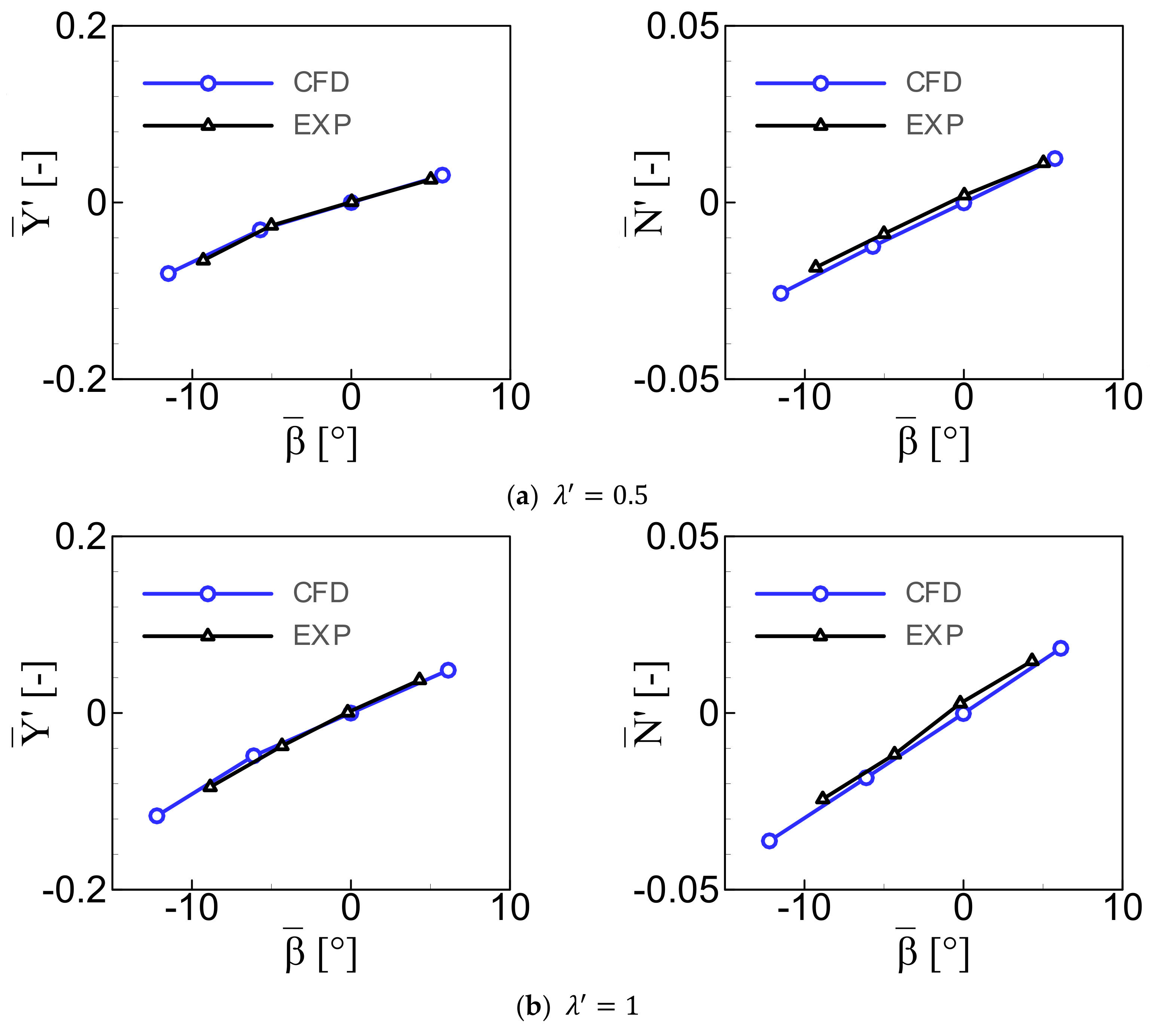
. A few head and beam waves (five wave lengths and one wave amplitude) are taken into account. The non-dimensional wave lengths λ are 0.5 ,   0.7 ,   1 ,   1.2 ,   and   1.5 , and the non-dimensional wave amplitude A is 0.01 , where λ and A are defined by λ / L p p and A / L p p , respectively.
The above case setup accords with that in the experiment by Yasukawa [12]. In addition, a virtual spring system consisting of one longitudinal spring and two transverse springs is attached to the ship model during RANS computations, according to the test conditions in the towing tank as well. The longitudinal spring with stiffness 529.2 N/m is attached at the center of gravity, and the two transverse springs with stiffness 313.6 N/m are attached at the positions 1.15 m and 1.22 m before and behind the center of gravity, respectively.

2.2. RANS Method

A right-handed Cartesian coordinate system in the horizontal plane is used to describe the flow around the ship. When the ship is at rest in calm water, the origin is positioned at the intersection of the mid-ship sections and the water’s surface, with the x -axis forward, the y -axis starboard, and the z -axis vertically downwards (see the coordinate system o - x y z shown in Figure 1). Because the horizontal coordinate system is always fixed during RANS computations, in order to simulate the ship oblique motion, the uniform oblique flow relative to the ship is set on the far-field boundaries. However, the available method of dynamic grid deformation is used to allow the ship to perform 6DOF motions in space due to the actions of the waves and spring system.
Under the assumption of an incompressible Newtonian fluid, the conservation equations of mass (continuity equation) and momentum (RANS equation) can be expressed as
U i x i = 0
U i t + U i U j x j = 1 ρ P x i + x j ν U i x j + U j x i U i U j ¯ ,
where x i = x ,   y ,   z and U i = U ,   V ,   W are independent Cartesian coordinates and flow velocity components, respectively; ρ is the fluid density; ν is the kinematic viscosity coefficient; P is pressure; and ρ U i U j ¯ is the Reynolds stress tensor.
According to the Bousinesq hypothesis, the specific Reynolds stress is assumed to be
U i U j ¯ = ν t U i x j + U j x i 2 3 δ i j k ,
where ν t is the eddy viscosity; k is the turbulent kinetic energy; and δ i j is the Kronecker symbol.
The k - ω SST turbulence model [13] is employed to approximate the eddy viscosity in Equation (4), where SST is the acronym of Shear-Stress-Transport, and ω is the specific dissipation rate. The method of VOF (Volume of Fluid) is applied to capture the free surface of the water–air flow.
The computational domain is limited by a box, which ranges from 2.5 L p p to 1.5 L p p along the longitudinal direction, from 2.0 L p p to 1.0 L p p along the transverse direction, and from 1.0 L p p to 1.0 L p p along the vertical direction. Computational grids are generated by using the commercial software Hexpress. Figure 2 presents a grid arrangement. The beam waves in the present consideration propagate from the starboard side to the port side. The longitudinal and transversal cell size is expanded downstream of the wave propagation, as seen in Figure 2. The purpose of the cell size expansion is to reduce the cell number, and to dampen the wave amplitude downstream.
Because wall functions are employed to model the flow in the boundary layer, the spacing of the first grid point to the hull surface is justified to satisfy the use condition that the near-wall points locate in the log-layer (usually the dimensionless distance y + . is more than 30) after a few pre-computations. The present mean y + is around 80. For resistance, the ITTC (International Towing Tank Conference) committee of resistance recommends that y + should range from 30 to 300.
In this study, a new module of the wave boundary condition was programed into OpenFOAM. The method of prescribing flow values on the far domain boundaries is employed to generate waves in the computational domain. In the horizontal coordinate system, the freestream flow velocity in the far field is superposed by the uniform oblique flow velocity, i.e., u 0 cos β 0 ,   u 0 sin β 0 ,   0 , and the wave orbital velocity from the solution of the potential theory of linear waves. If freestream wave evaluation is expressed as
ζ = A sin ω e t + k w x cos χ 0 + k w y sin χ 0 ,
the velocity components of the freestream flow are
U f = u 0 cos β 0 A ω 0 cosh k w h z sinh k w h sin ω e t + k w x cos χ 0 + k w y sin χ 0 cos χ 0
V f = u 0 sin β 0 A ω 0 cosh k w h z sinh k w h sin ω e t + k w x cos χ 0 + k w y sin χ 0 sin χ 0
W f = A ω 0 sinh k w h z sinh k w h cos ω e t + k w x cos χ 0 + k w y sin χ 0 ,
where k w is the wave number and ω 0 is the natural frequency of the waves.
The four far boundaries at x = 2.5 L p p , L p p and y = L p p , 2 L p p are considered to be wave boundaries, on which the wave evaluation and flow velocities are specified by Equation (5) and Equations (6)–(8), respectively. In order to prevent wave reflection, relaxation zones adjacent to these boundaries are set up. A relaxation function α R l d is applied inside the relaxation zones. The function expression [14] is below.
α R l d = 1 e l d 3.5 1 e 1 ,
where l d 0 , 1 is the relative distance, as illustrated in Figure 3. l d is always zero at the interface between the non-relaxed part of the computational domain and the relaxation zone, and 1 at the wave maker boundary. α R varies from 0 to 1, depending on l d .
During RANS computations, the wave evaluation and flow velocity in the relaxation zone are updated at each time step in the following way:
Φ = α R Φ computed + 1 α R Φ taget ,
where Φ is either the flow velocity component or the wave evaluation; Φ computed is the value from RANS; and Φ taget is the freestream value prescribed by Equation (5) or Equations (6)–(8).
The bottom boundary at z = L p p is set as a free slip wall. The top boundary at z = L p p is set as a pressure outlet. The boundary types are listed in Table 2.
The RANS solver in OpenFOAM is based on a finite volume technique which permits the use of arbitrary polyhedral grids, including hexahedron, tetrahedron, and prism, etc. A suite of basic discretization schemes and solution algorithms are available. In the present applications, a second-order upwind difference scheme (UDS) and a central difference scheme (CDS) are selected to approximate the convective terms and diffusive terms, respectively. A second-order backward scheme is applied for time discretization. Turbulence is discretized with the second-order UDS. The systems of linear equations resulting from the discretization are solved by using iterative solvers, which here are Gauss-Seidel relaxation for the velocity, k and ω, and a Generalized Geometric Multi-Grid (GAMG) for pressure. The PIMPLE algorithm, which merges the PISO (Pressure Implicit with Splitting of Operators) and SIMPLE (Semi-Implicit Method for Pressure-Linked Equations) algorithms, is applied to couple the mass and momentum equations. More details about boundary conditions and numerical settings can be found in the previous publication by Yao et al. [15].
Besides this, in order to improve the numerical stability, the virtual wave maker is inactivated at the beginning, i.e., in calm-water conditions, until it reaches a steady flow. The calm-water simulation lasts for 100 s. Afterwards, the wave generation starts. For each case, around 2000 time steps per encounter period are performed, and ten outer-loop iterations are carried out during each time step. Each simulation runs for more than 20 encounter periods.

2.3. Post-Processing

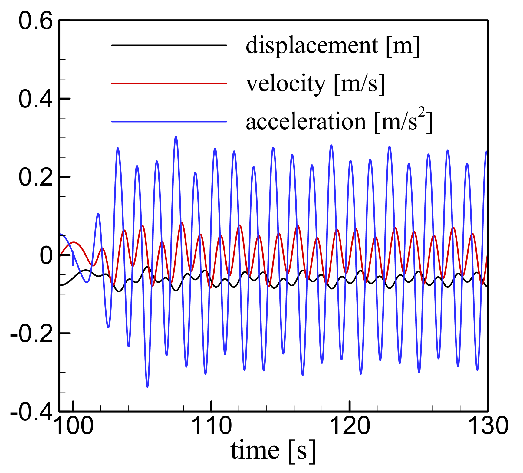
The forces and moments directly from RANS are obtained by integrating the pressure and viscous stress over the hull surface. The pressure is the total pressure, including the dynamic pressure and static pressure. In the present consideration, the forces and moments, as well as the ship motions, are evaluated at the center of gravity in the completely ship-fixed coordinate system. This means that the results from RANS have to be transformed from the horizontal coordinate system to the ship-fixed coordinate system during the data post-processing. The low-frequency components and high-frequency components of force, moment or motion can be extracted by regressing the time histories of the RANS results. Figure 4 presents the computed time histories of the displacement, velocity and acceleration of the surge motion for a case. The surge displacement contains the initial longitudinal elongation of the spring system which produces a force to balance the ship resistance in calm water. As observed, the traces are explicitly characterized by two different periods. One is excited by waves, which is definitely consistent with the wave period. The other is due to the spring system, and larger than the wave-induced one. In order to separate out the low-frequency component and high-frequency component from the time histories, Fourier series with double frequencies, i.e., Equation (1), are employed to regress the time histories. The Fourier series taken here are up to the fifth order. The spring frequency ω s obtained from regression analysis is around 1.604 s−1, corresponding to a period of 3.92 s.
During the towing tank test, the aforementioned forces and moments obtained by integrating the pressure and viscous stress over the hull surface cannot be directly measured, as the ship performs inertia motions in the waves. The inertia forces and moments are naturally included in the measured data. In this regard, it is very similar to the PMM (Planar Motion Mechanism) test or CMT (Circular Motion Test). For comparison purposes, we can first subtract the inertia forces and moments from the directly measured data of the PMM test or CMT, then compare the resulting data with the computed results for validation. The works by Uharek and Cura-Hochbaum [16] and Lengwinat and Cura Hochbaum [17] confirmed the contributions of inertia effects to the mean forces and moments acting on a ship in waves. The inertia forces and moments are not of small values for some cases, compared with that obtained by integrating the pressure and viscous stress over the hull surface.
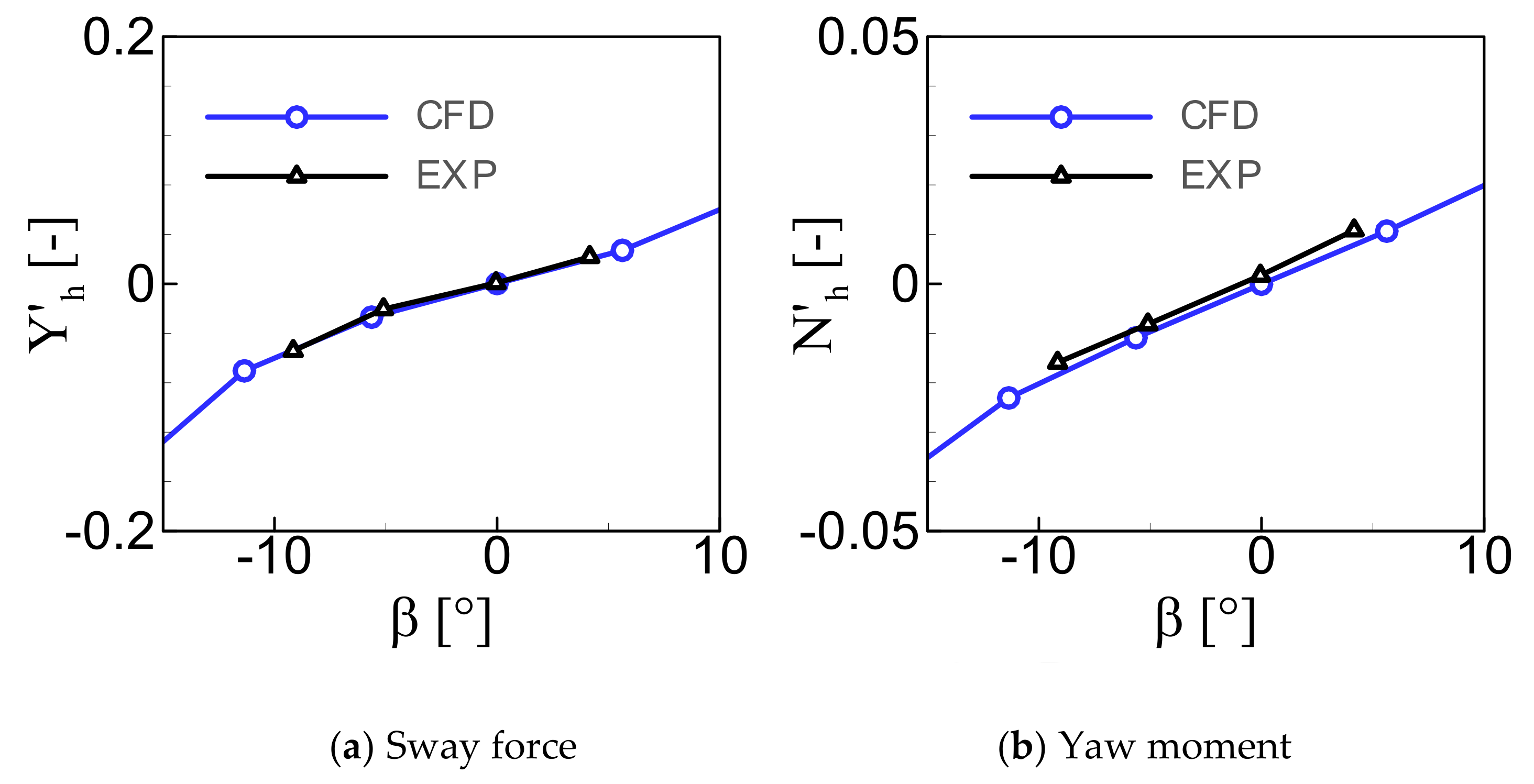
In order to validate the present computed results, they are compared with the experimental data published by Yasukawa [12]. The experimental data should include the inertia effects. The mean surge force, sway force and yaw moment, including inertia effects, may be expressed in a ship-fixed coordinate system as
X ¯ = X ¯ h m u ˙ ¯ + m v r ¯ m w q ¯ + m g T ¯ 31
Y ¯ = Y ¯ h m v ˙ ¯ + m w p ¯ m u r ¯ + m g T ¯ 32
N ¯ = N ¯ h I z r ˙ ¯ I y I x p q ¯ ,
where m is the ship mass; I x , I y and I z are inertia moments and I y = I z is assumed; g is the acceleration due to gravity; X h , Y h and N h are the force or moment due to both hydrodynamics and hydrostatics; u , v and w are components of ship linear velocity; p , q and r are components of ship angular velocity; T is the transformation matrix; and T 31 is the component at the third row of first column. The dot over a variable denotes a derivative with respect to time, and the bar over a variable denotes the mean of the variable.
For the data post-processing, the forces, moments and ship motions directly from RANS are first transformed from the horizontal coordinate system to the ship-fixed coordinate system, as mentioned. Then, Equation (1) is used to regress the resulting data, and X ¯ h , Y ¯ h , N ¯ h , u ˙ ¯ , v ˙ ¯ and r ˙ ¯ can be consequently obtained. For the mean terms of two coupling motion variables, such as v r ¯ , the time histories of their product are calculated at first, and then the resulting time histories are regressed using Equation (1).

3. Results and Analysis

In order to ensure enough grid resolution, grid dependency analysis is carried out for the case λ = 1 and β 0 = 10 ° in head-wave conditions. Coarse, medium and fine grids with around 0.26, 1.69 and 10.52 million cells are generated, respectively, by systematically doubling the cell size in three dimensions. As mentioned, during RANS computations, the virtual wave maker is inactive within the first 100 s, i.e., in calm-water condition, then afterwards wave generation starts. Table 3 presents the computed surge force, sway force and yaw moment in calm water using the three grids. As seen in the table, the change of force or moment becomes smaller with the increasing grid resolution. The maximum discrepancy between the results on the medium grid and fine grid is below 3%. The segments of the computed time histories of the surge force, sway force and yaw moment after activating the wave maker are shown in Figure 5, and the RMSE (Root-Mean-Square Error) is presented in Table 4. Note that the forces and moment in the figure are due to hydrodynamics and hydrostatics, without including inertia effects. The time traces also display the tendency towards convergence, as desired. The medium grid seems to be of enough resolution for the selected case. In order to reduce the computational time, the medium grid is therefore used for the other cases considered.
Figure 6 shows a comparison of the computed calm-water sway force and yaw moment with the experimental data. The force and moment are made non-dimensional by 0.5 ρ u 0 2 L p p 2 and 0.5 ρ u 0 2 L p p 3 , respectively. Very good agreement can be observed. It should be noted that the real oblique angle β in calm water or the mean oblique angle β ¯ in waves is a sum of β 0 and β , as mentioned, and β is obtained from RANS. Figure 7 shows β versus β 0 . As seen, β is almost proportional to β 0 in both clam water and waves. The change rate of β to β 0 becomes larger in waves, especially in head waves, compared with that in calm water.
The computed mean sway force and yaw moment with inertia effects for three head waves are compared with the experimental data in Figure 8. Most of the results show excellent agreements with the available experimental data. The errors for the yaw moments at λ = 1.5 are a little bit larger. The reason is as-yet unknown.
The comparisons of the numerical added resistance and RAOs (Response Amplitude Operator) of surge, heave and pitch for β 0 = 0 ° in head waves with the experimental data are presented in Figure 9. The added resistance is computed by subtracting the calm-water resistance from the mean resistance with the contributions of the inertia effects in the waves, and is made non-dimensional by ρ g A 2 B 2 / L p p , where B is the ship breadth. For short waves, i.e., λ = 0.5 ,   0.7 , the computed added resistances agree quite well with the experimental data. However, the added resistances for long waves are overestimated. Overestimation for surge RAOs is observed for long waves as well. Nevertheless, the computed RAOs of heave and pitch generally show fairly good agreements with the experimental data for both short and long waves.
The oblique angle β 0 has non-negligible influences on added resistance, especially for long waves, as shown in Figure 10. For a larger β 0 , the added resistance decreases in general, especially in long waves. The influences may be due to the different mean oblique angle β ¯ and the different mean encounter wave angle χ ¯ , as β ¯ = β 0 + β and χ ¯ = χ 0 + χ , where β and χ are related to β 0 and the wave length. However, these seem not to affect the RAOs of surge, heave and pitch (see Figure 10), as the curves of the RAO versus the wave length are almost coincident, although β 0 is different.
The RAOs of sway, roll and yaw in head waves at λ = 1 ,   1.5 are presented in Figure 11. When β 0 = 0 ° , both β and β ¯ are theoretically zero in head waves, and the RAOs of sway, roll and yaw are zero, as expected. The computed results show general good agreements with the experimental data. The wave length does not influence the RAOs of sway and yaw; however, the roll RAOs at λ = 1.5 become larger, compared with that at λ = 1 . In addition, the sway RAOs are generally of small value compared with the heave RAOs shown in Figure 9, and the yaw RAOs are also of small value compared with the pitch RAOs shown in Figure 9.
The computed mean sway force and yaw moment for three beam waves are compared with the experimental data in Figure 12. Very excellent agreements are found as well. Figure 13 presents the comparison of the computed motion RAOs in beam waves with the experimental data for λ = 1 ,   1.2   and   1.5 . It is observed that the computed RAOs of surge, sway, heave and pitch generally agree well with the experiments, whereas the errors for roll and yaw are large. Computations underestimate the RAOs of roll and yaw. Compared with the situation in head waves, sway RAOs in beam waves increase prominently.
Figure 14 presents the wave snapshots for S-175 performing straight head motion and oblique motion in head waves. For β 0 = 10 ° , the wave surface on the starboard side is squeezed due to the ship’s oblique motion. Green water on bow deck is observed. In addition, wave reflection from the side boundaries is not found, which indicates that the used method of generating waves works quite well.

4. Concluding Remarks

This article presents a study on the computation of the mean forces and moments, as well as the 6DOF motions, for a ship moving obliquely in regular head and beam waves. The RANS technique based on OpenFOAM is employed for this purpose. Great efforts have been made towards the implementation of new wave boundary conditions, and the post-processing of the RANS results. This shows that the computed mean surge force, sway force and yaw moment with the contributions of inertia effects generally agree quite well with the experimental data, which confirms the inertia effects due to waves. The computed motion RAOs show reasonable agreement with the experimental data as well. This explicitly demonstrates the reliability of the RANS solver and the correctness of the data post-processing.
To separate out the low-frequency component and high-frequency component of force, moment or motion purely induced by waves remains challenging, as the disturbances from the spring to the components always exist. The influences of the spring on the forces, moments and ship motions should be carefully investigated in the future. For numerical computations, in order to avoid the influences of the spring, constant forces and moments, which can offset the slow drift effects of waves right, could be added into ship motion equations during motion prediction. If so, the ship is able to oscillate around a certain potion in space, without a spring constraint. Nevertheless, a new problem may arise, as the required constant forces and moments are unknowns in advance.

Author Contributions

Conceptualization, J.Y.; methodology, J.Y.; software, J.Y.; validation, J.Y.; formal analysis, J.Y.; investigation, J.Y. and C.Z.; data curation, J.Y.; writing—original draft preparation, J.Y.; writing—review and editing, J.Y. and X.S.; supervision, Z.L.; project administration, X.C.; funding acquisition, Z.L. All authors have read and agreed to the published version of the manuscript.

Funding

This research was funded by the National Natural Science Foundation of China, grant numbers 51720105011, 51609188.

Institutional Review Board Statement

Not applicable.

Informed Consent Statement

Not applicable.

Data Availability Statement

The data used to support the findings of this study are available from the corresponding author upon request.

Conflicts of Interest

The authors declare no conflict of interest.

References

  1. Carrica, P.M.; Ismail, F.; Hyman, M.; Bhushan, S.; Stern, F. Turn and Zigzag Manoeuvres of a Surface Combatant Using a URANS Approach with Dynamic Overset Grids. J. Mar. Sci. Technol. 2013, 18, 166–181. [Google Scholar] [CrossRef]
  2. Yasukawa, H. Simulation of Wave-Induced Motions of a Turning Ship. J. Jpn. Soc. Nav. Archit. Ocean. Eng. 2006, 4, 117–126. (In Japanese) [Google Scholar]
  3. Yasukawa, H. Simulations of Ship Manoeuvring in Waves (1st report: Turning motion). J. Jpn. Soc. Nav. Archit. Ocean. Eng. 2006, 4, 127–136. (In Japanese) [Google Scholar]
  4. Skejic, R.; Faltinsen, O.M. A Unified Seakeeping and Manoeuvring Analysis of Ships in Regular Waves. J. Mar. Sci. Technol. 2008, 13, 371–394. [Google Scholar] [CrossRef]
  5. Zhang, W.; Zou, Z.; Deng, D. A Study on Prediction of Ship Manoeuvring in Regular Waves. Ocean. Eng. 2017, 137, 367–381. [Google Scholar] [CrossRef]
  6. Lee, J.; Nam, B.W.; Lee, J.H.; Kim, Y. Development of Enhanced Two-Time-Scale Model for Simulation of Ship Manoeuvring in Ocean Waves. J. Mar. Sci. Eng. 2021, 9, 700. [Google Scholar] [CrossRef]
  7. Yao, J.; Liu, Z.; Song, X.; Su, Y. Pure low-frequency and pure high-frequency ship motion equations in regular waves. Ocean Eng. 2021, 233, 109152. [Google Scholar] [CrossRef]
  8. Yasukawa, H.; Hirata, N.; Matsumoto, A.; Kuroiwa, R.; Mizokami, S. Evaluations of wave-induced steady forces and turning motion of a full hull ship in waves. J. Mar. Sci. Technol. 2019, 24, 1–15. [Google Scholar] [CrossRef]
  9. Zhang, W.; el Moctar, O.; Schellin, T.E. Numerical study on wave-induced motions and steady wave drift forces for ships in oblique waves. Ocean Eng. 2020, 196, 106806. [Google Scholar] [CrossRef]
  10. Zhu, Z.; Lee, J.H.; Kim, Y. CFD Analysis of Ship Oblique Towing in Waves. In Proceedings of the 11th International Workshop on Ship and Marine Hydrodynamics, Hamburg, Germany, 22–25 September 2019. [Google Scholar]
  11. Uharek, S. Numerical Prediction of Ship Manoeuvring Performance in Waves. Ph.D. Thesis, Technical University of Berlin, Berlin, Germany, 2019. [Google Scholar]
  12. Yasukawa, H.; Faizul, A.A. Experimental Study on Wave-Induced Motions and Steady Drift Forces of an Obliquely Moving Ship. J. Jpn. Soc. Nav. Arch. Ocean Eng. 2006, 3, 133–138. [Google Scholar] [CrossRef]
  13. Menter, F.R.; Kuntz, M.; Langtry, R. Ten Years of Industrial Experience with the SST Turbulence Model. In In Proceedings of the Turbulence, Heat and Mass Transfer 4, Antalya, Turkey, 12–17 October 2003. [Google Scholar]
  14. Jacobsen, N.G.; Fuhrman, D.R.; Fredsøe, J. A wave generation toolbox for the open-source CFD library: OpenFoam®. Int. J. Numer. Methods Fluids 2012, 70, 1073–1088. [Google Scholar] [CrossRef]
  15. Yao, J.; Liu, Z.; Su, Y.; Cheng, X.; Song, X.; Zhan, C. A Time-Averaged Method for Ship Maneuvering Prediction in Waves. J. Ship Res. 2020, 64, 203–225. [Google Scholar] [CrossRef]
  16. Uharek, S.; Cura-Hochbaum, A. The influence of inertial effects on the mean forces and moments on a ship sailing in oblique waves Part B: Numerical prediction using a RANS code. Ocean Eng. 2018, 165, 264–276. [Google Scholar] [CrossRef]
  17. Lengwinat, A.; Cura-Hochbaum, A. The influence of inertial effects on the mean forces and moments on a ship sailing in oblique waves part A: A new measurement device for wave forces. Ocean Eng. 2018, 166, 1–11. [Google Scholar] [CrossRef]
Figure 1. Illustration of a ship towed obliquely in regular beam waves.
Jmse 09 01176 g001
Figure 2. Grid arrangement.
Jmse 09 01176 g002
Figure 3. A sketch of the relaxation zone.
Jmse 09 01176 g003
Figure 4. Surge displacement, velocity and acceleration.
Jmse 09 01176 g004
Figure 5. Grid dependency analysis.
Jmse 09 01176 g005
Figure 6. Sway force and yaw moment versus β in calm water.
Jmse 09 01176 g006
Figure 7. β versus β 0 based on RANS.
Jmse 09 01176 g007
Figure 8. Mean sway force and yaw moment versus the mean oblique angle in head waves.
Jmse 09 01176 g008aJmse 09 01176 g008b
Figure 9. Added resistance and RAOs of the surge, heave and pitch for β 0 = 0 ° in head waves.
Jmse 09 01176 g009
Figure 10. Computed added resistance and RAOs of surge, heave and pitch for different β 0 in head waves.
Jmse 09 01176 g010
Figure 11. RAOs of sway, roll and yaw versus mean the oblique angle in head waves.
Jmse 09 01176 g011
Figure 12. Mean sway force and yaw moment versus the mean oblique angle in beam waves.
Jmse 09 01176 g012
Figure 13. Motion RAOs versus the mean oblique angle in beam waves.
Jmse 09 01176 g013aJmse 09 01176 g013b
Figure 14. Wave snapshots for S-175 in head waves λ = 1 .
Jmse 09 01176 g014
Table 1. Principal dimensions of S-175.
ItemsReal ShipModel for CFD (1:50)
L p p [m]175.003.500
B [m]25.400.508
T [m]9.50.190
C b 0.5720.572
x G [m]−2.55−0.051
G M ¯ [m]1.250.025
K M ¯ [m]10.50.21
i x / B 0.338
i z / L p p 0.272
Table 2. Boundary conditions.
BoundaryType
x = 2.5 L p p , L p p and y = L p p , 2 L p p wave boundary
z = L p p slip
z = L p p outlet
Table 3. Grid dependency analysis for oblique motion at β 0 = 10 ° in calm water.
GridSurge ForceSway ForceYaw Moment
Value [N]Diff (%)Value [N]Diff (%)Value [Nm]Diff (%)
coarse−4.288.35−20.1411.46−23.5413.45
medium−3.952.47−18.071.98−20.752.93
fine−4.05−17.72−20.16
Table 4. RMSE of the grid dependency analysis, as shown in Figure 4.
Grid X h Y h N h
coarse1.57012.48392.4549
medium0.26510.86361.0873
fine
Publisher’s Note: MDPI stays neutral with regard to jurisdictional claims in published maps and institutional affiliations.

