1. Introduction
Wind waves during propagation, especially in coastal zones, are subject to various changes associated primarily with the impact of nonlinear and dissipative processes. As shown by modern theoretical and experimental studies, the nonlinear processes are dominant for wave evolution both in deep and shallow water (for example, [
1,
2,
3]). Wave transformation leads to changes in the shape of the wave spectrum. Sometimes, the major peak frequency shifts to the low-frequency region—where so-called “frequency downshifting” is observed [
4,
5,
6,
7]. It is not completely understood in detail how the frequency downshift occurs. For example, is the process continuous or discrete? For deep water waves, a downshifting mechanism due to the development of Benjamin–Feir instability was proposed [
5]. It occurs discretely with a frequency step equal to the difference between the peak frequency and the most unstable low-frequency mode. Dissipation of wave energy during wave propagation accelerates the downshift of the peak frequency [
7,
8]. As shown by numerical and laboratory experiments, for steep waves, a cascade frequency downshift is possible, and that occurs at a spatial distance of less than 10 wavelengths. As a result of numerical modeling, it was noted that the downshifting process for waves at deep and intermediate water depths are different [
9]. The frequency downshift in wave spectra of shallow water is not observed always and the detailed mechanism is still not known. In most studies, it is assumed that this is the result of wave breaking and dissipation of wave energy in the high-frequency part of the spectrum. However, as was shown experimentally and numerically for the spatial evolution of frequency spectra of unidirectional narrow-banded waves (breaking and non-breaking) in deep water, frequency downshifting is explained by nonlinear energy transfer and the breaking processes are not necessarily responsible for it [
4]. Laboratory and numerical experiments with waves in shallow water have shown the importance of the shape of the initial spectrum for the frequency downshifting that is also an indirect confirmation of the main role of nonlinear processes [
6].
If we assume that nonlinearity is the main factor contributing to the downshifting, then the conditions for wave transformation in shallow water are important in which nonlinear processes will clearly manifest themselves, demonstrating all the effects. As noted in [
10], waves traveling a long distance over a very low sloping bottom will undergo more nonlinear evolution than those traveling over a steep sloping bottom, so the features of wave nonlinearity will depend on the propagation distance and water depth. In particular, additional frequency peaks can be formed due to spectrum broadening as a result of the backward transfer of energy from higher frequencies [
11] and lower (infragravity) frequencies to the main peak [
12]. The authors of [
12] analyzed in detail the occurrence of frequencies below the main peak due to three-wave interactions with frequencies of the infragravity range during the evolution of the wave spectrum at a shallow water depth above a mild and low bottom slope. In the studies presented in [
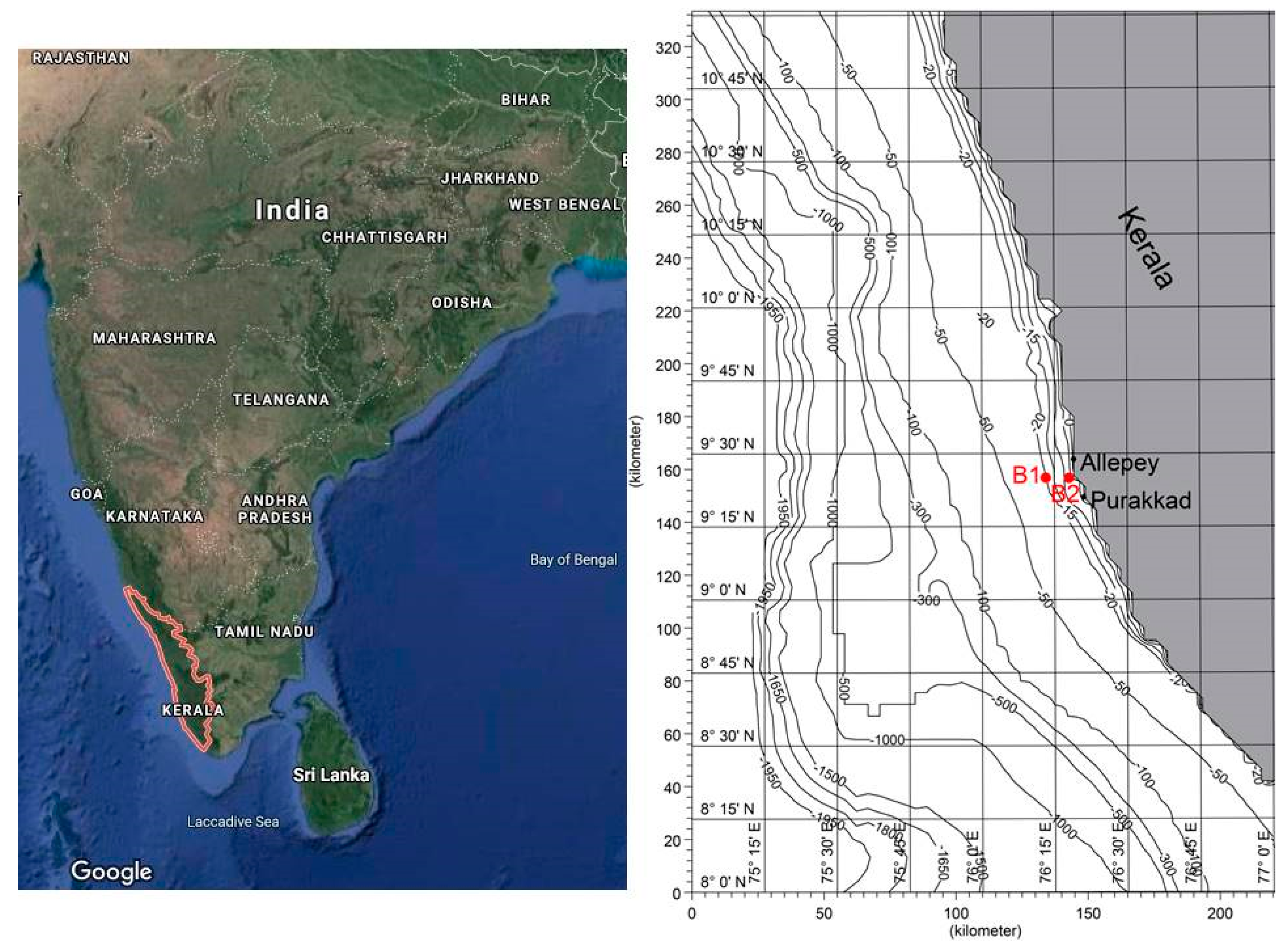
12], this peak does not become dominant. Therefore, short traveling over a sloping bottom or a steep slope could be the reason for why the frequency downshift in coastal zones is not observed regularly. However, there are areas where waves travel long distances over an almost flat bottom, for example, off Kerala, along the southwest coast of India. This region has a very low mild sloping bottom: waves traveling towards the shore bottom slope could be in the range 0.0007–0.0001 within 5–10 kms (
Figure 1). The Kerala coast is characterized by the presence of mudbanks, that form and exist during the southwest monsoon (May–September) period. As a natural phenomenon, mudbanks are of great importance for the economy, because they attract fish feeding on benthos and algae accumulating on banks and create calm wave conditions for fishing. General mechanisms for the formation of mudbanks are muddy bottom erosion and fluidization at intermediate water depth under the high waves during the monsoon period and then transport of fluid mud by waves and currents to the nearshore region where the localization of the mudbanks depend on wave refraction [
13]. However, the peculiarities and full details of these mechanisms are still unknown.
A field experiment was conducted off Alleppey, Kerala, in May–July 2014, during mudbank occurrence along the coast (detailed description is given in [
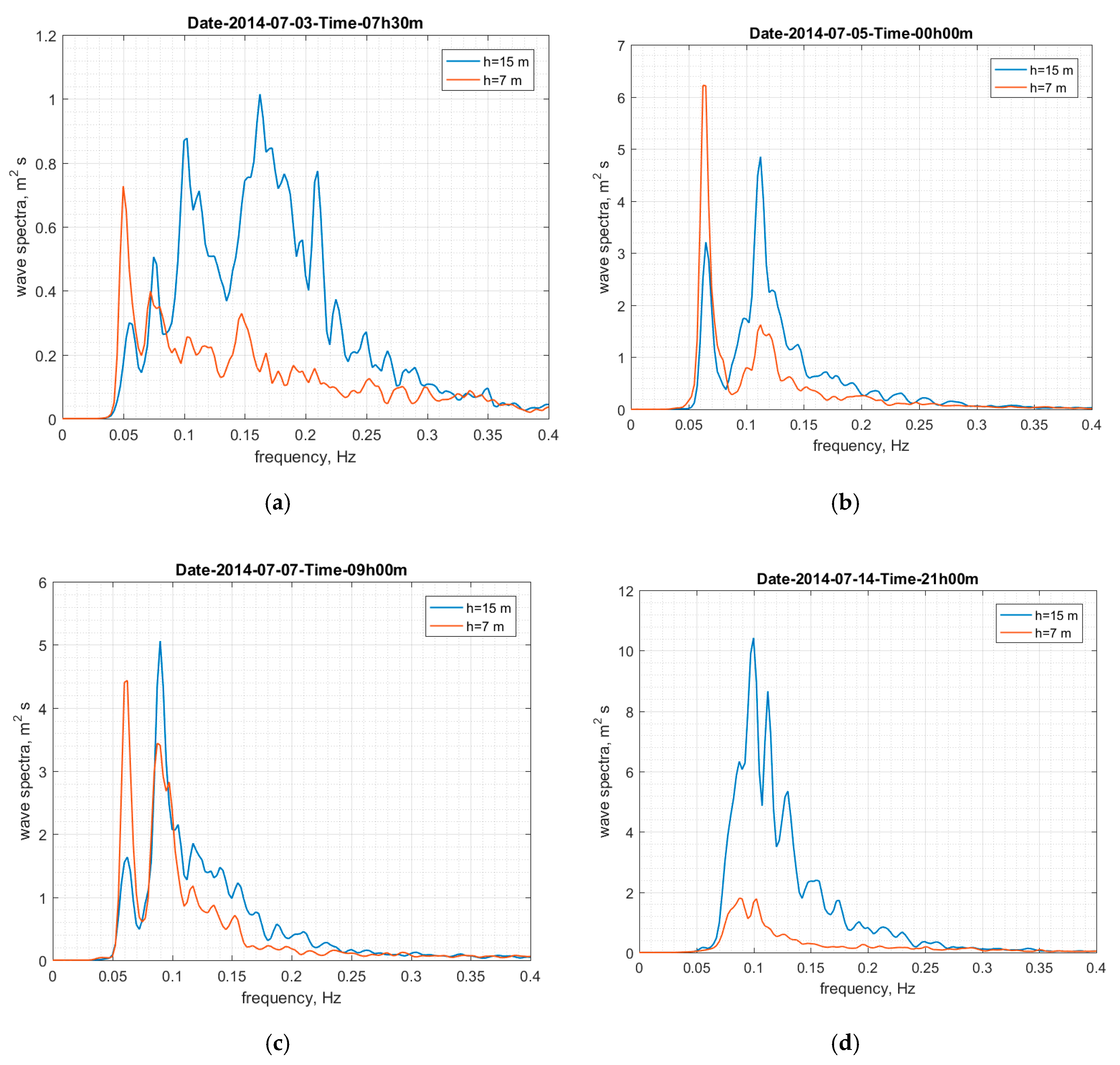
14]). A detailed analysis of wave spectral data showed that the wave spectrum follows a specific shape at both the field locations B1 and B2 (
Figure 1). It was observed that there is an additional frequency peak down the main peak of the wave spectrum and as the waves approach the shore, this peak becomes the main one, i.e., frequency downshifting occurs [
14]. Typical examples of such spectra calculated on wave chronograms measured by the Datawell buoys at water depths of 15 and 7 m are shown in
Figure 2. Similar wave spectra with two peaks off the Kerala coastal zone are presented in [
15].
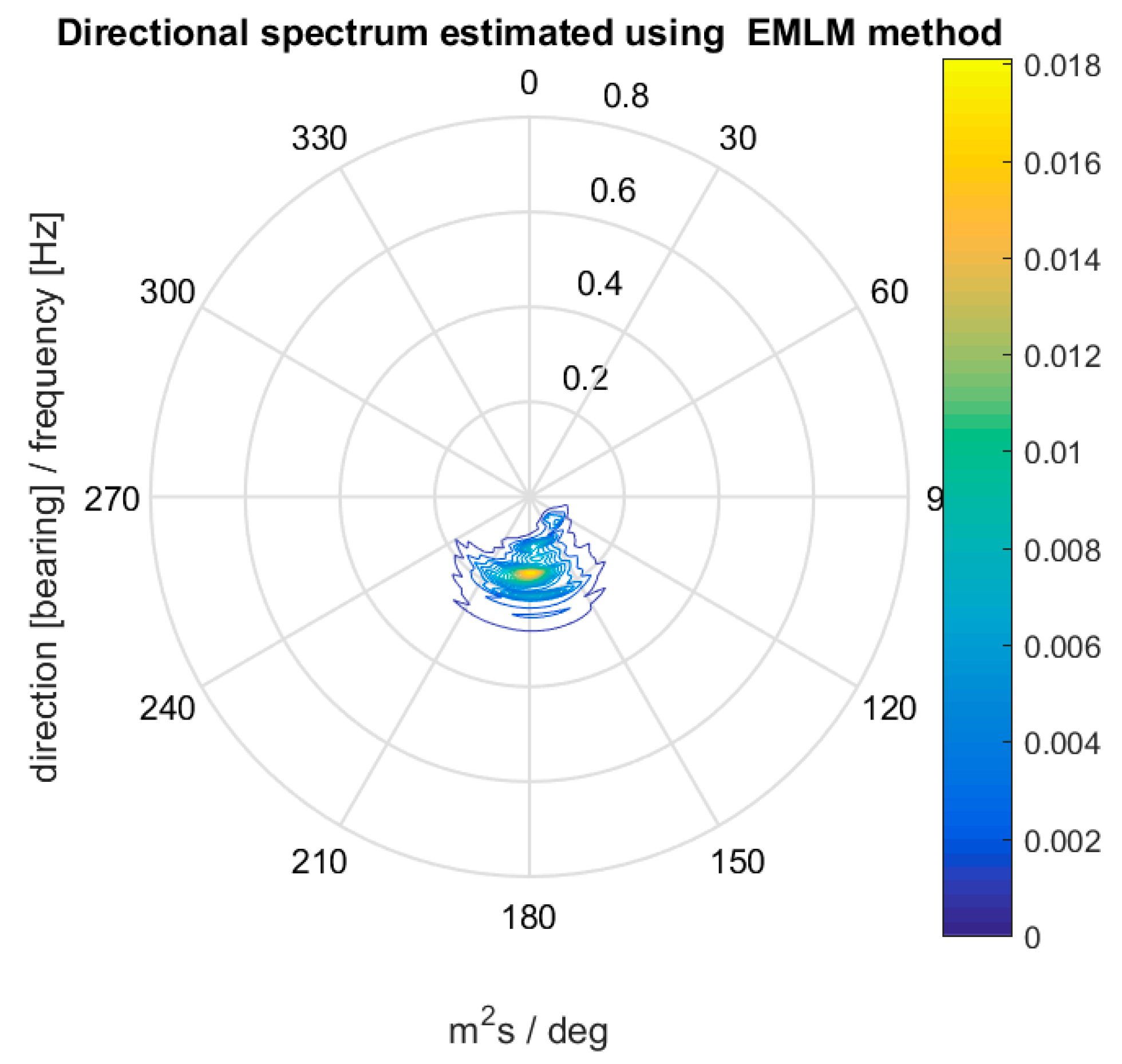
The genesis of this low-frequency peak is often interpreted as the presence of swell waves at mixed sea state. However, calculated directional wave spectra of wave regimes (
Figure 2) demonstrated that the wind seas and swells have the same directions (
Figure 3).
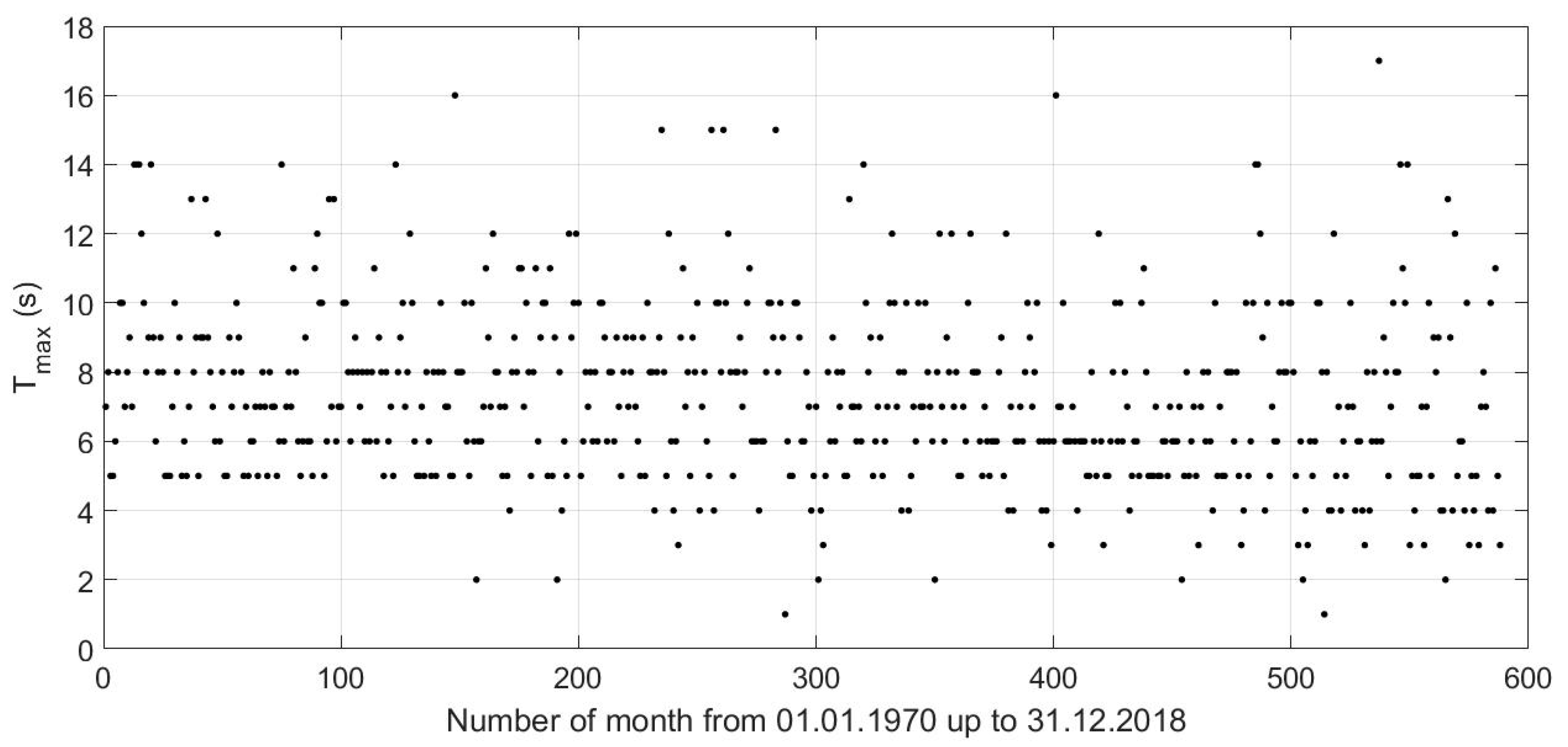
The experimental spectral data at both the locations showed that this low-frequency spectral peak (“swell”) corresponds to waves with periods of 16–18 s. However, the wave data of Voluntary Observing Ships taken from the Global Atlas of Ocean waves [
16,
17] over the past 49 years in the area of the Kerala coast demonstrated that swell with such periods is sparsely observed (
Figure 4).
Both these facts indicate that the low-frequency peaks of the spectrum do not indicate the presence of swells but instead they might have been formed during the nonlinear transformation of waves over a relatively long distance in shallow water with a very low slope between 15 and 7 m depths.
Based on the above observations, the main aim of this study is (1) to prove the nonlinear mechanism of low-frequency spectral peak formation and the downshift of the spectral maxima on its frequency position during wave propagation over a very low sloping bottom of the Kerala coast and (2) to investigate the role of the frequency downshifting effect in the mechanism of mudbanks formation in this region.
2. Methods
The nonlinear wave evolution in intermediate and shallow water depths corresponding to conditions of the Kerala coastal zone, as mentioned earlier, was provided by three wave interactions. To fix the nonlinear relationships between wave harmonics, bicoherence (b) and bispectrum (B) were calculated by formulas [
18]
where
is the averaging operator,
is the Fourier transform of the free surface elevations and
f is the frequency. The bicoherence value indicates what part of energy of harmonic
can be referenced as the result of the triad interaction. The bispectrum is a statistical demonstration of the contribution of the triad interaction to the
wave component.
As the Datewell buoys mentioned above have built-in filtering at the level of 0.025 Hz and low-frequency components of waves are filtered out, the low-frequency harmonics (infragravity waves) with frequencies between 0.01 and 0.03 Hz can play a significant role in the nonlinear wave transformation processes [
12,
19]. To investigate further, we planned to use the method of numerical modeling.
For wave modeling, the SWASH model was applied. SWASH is an open source numerical model, suitable for simulating wave transformation from the offshore regions to the beach [
20]. It is a phase-resolving wave model based on non-hydrostatic equations with mass and momentum conservation [
21,
22]. SWASH can be run either in depth-averaged or in multi-layered mode. In multi-layered mode, the computational domain is divided into a fixed number of vertical terrain-following layers. SWASH improves its frequency dispersion by increasing the number of layers. In this case, layer-integrated velocity components are calculated for each layer [
23].
According to the field experiment, the conditions of wave propagation were quite uniform along the coast and the waves approach was predominantly in the normal direction. To decrease the model computational time, the simulations were done in 1D (flume-like) mode. Note that we did not try to reproduce the field conditions exactly, as the main interest was modeling the wave propagation on long distances over a practically constant or very small slope of the bottom.
The length of the rectangular equidistant computational grid was 5000 m and number of meshes was 499, and this setup gives 10 m steps on the distance. The computational time step was 0.01 s. Multi-layered mode (5 layers) was chosen to improve the wave dispersion characteristics of transforming waves. Two cases of wave transformation were simulated: (i) waves that propagated in clear water and (ii) in water with viscous mud as a case study for a mudbank. In the second case, the concentration of sediment in water was set to 1500 kg/m
3 (this value was taken from earlier studies [
14,
15]). The cohesive sediment transport option is enabled in the model to account for the presence of suspended sediments in water, but its parameters are tuned so that the concentration of sediments in water remains constant during simulation. The other parameters of the model were set as follows: constant horizontal eddy diffusivity is 10 m
2/s; critical bed shear stress for erosion is 1 N/m
2; critical bed shear stress for deposition is 0.5 N/m
2; entrainment rate for erosion is 0.0004 kg/m
2/s; fall velocity is 0.01 mm/s; Schmidt number for sediment is taken as default 0.7; and the empirical constant to reduce the Von Karman constant and thereby the bed shear stress in the sediment-laden bottom boundary layer as suggested in the manual is 5.5. The density effect of the suspended sediments is also included in the model. The standard k—ε turbulence model for the vertical mixing and the vertical logarithmic velocity profile near the bed surface is applied, as recommended in the manual [
20]. Both the initial water level and velocity components are set to zero.
As initial waves, we have used the JONSWAP spectra waves with the peak enhancement parameter as 1.0, the significant wave height as 1 m and the peak period as 10 s, and these values qualitatively correspond to the wave parameters of the field experiment. The evolution of waves was simulated at the constant depth of 7 m, and over a bottom slope of 0.0001, approximately corresponding to field conditions. A weakly reflective condition allowing outgoing waves was adopted to simulate incident waves without reflections at the “wavemaker” boundary. At the output boundary, a sponge layer was placed to absorb waves propagating outside the computational domain. Output parameters were extracted as free surface elevations in the following distances from the input boundary: 0, 500, 1000, 2000, 2500, 4000 and 4500 m. The length of the time series was 3000 s with a time step of 0.1 s. In all modeling tests, depth-induced wave breaking was not observed. Analysis of model data showed that the bottom slope of 0.0001 has a minor effect on the evolution of the wave spectrum. Therefore, in the subsequent model runs, the wave propagation at the constant depth only will be discussed. The validation of the model and its ability to adequately reproduce the transformation of waves has been tested repeatedly and a list of references can be found in the manual [
20]. In particular, the validation of nonlinear three-wave interactions during wave propagation in shallow water was carried out in [
12].
3. Results and Discussion
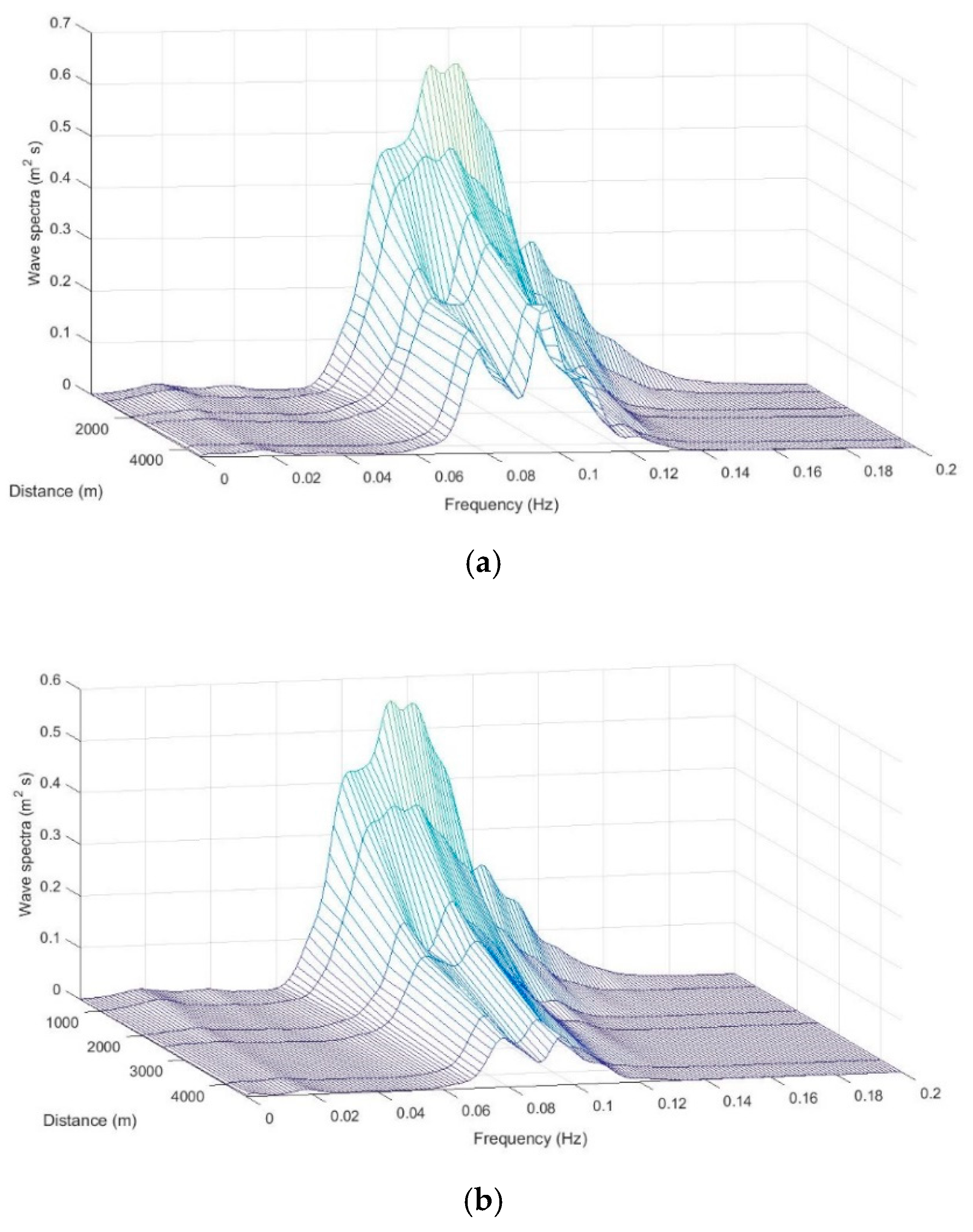
In
Figure 5, the evolutions of wave spectra in water and a viscous mud (or mudbank) are shown. It is clearly seen how the new peak at frequency 0.08 Hz arises and grows in addition to the initial spectral peak at 0.1 Hz. In the presence of mud, we observe that at the distance of 4000 m, the new peak becomes greater than the initial one which shows that frequency downshifting has occurred.
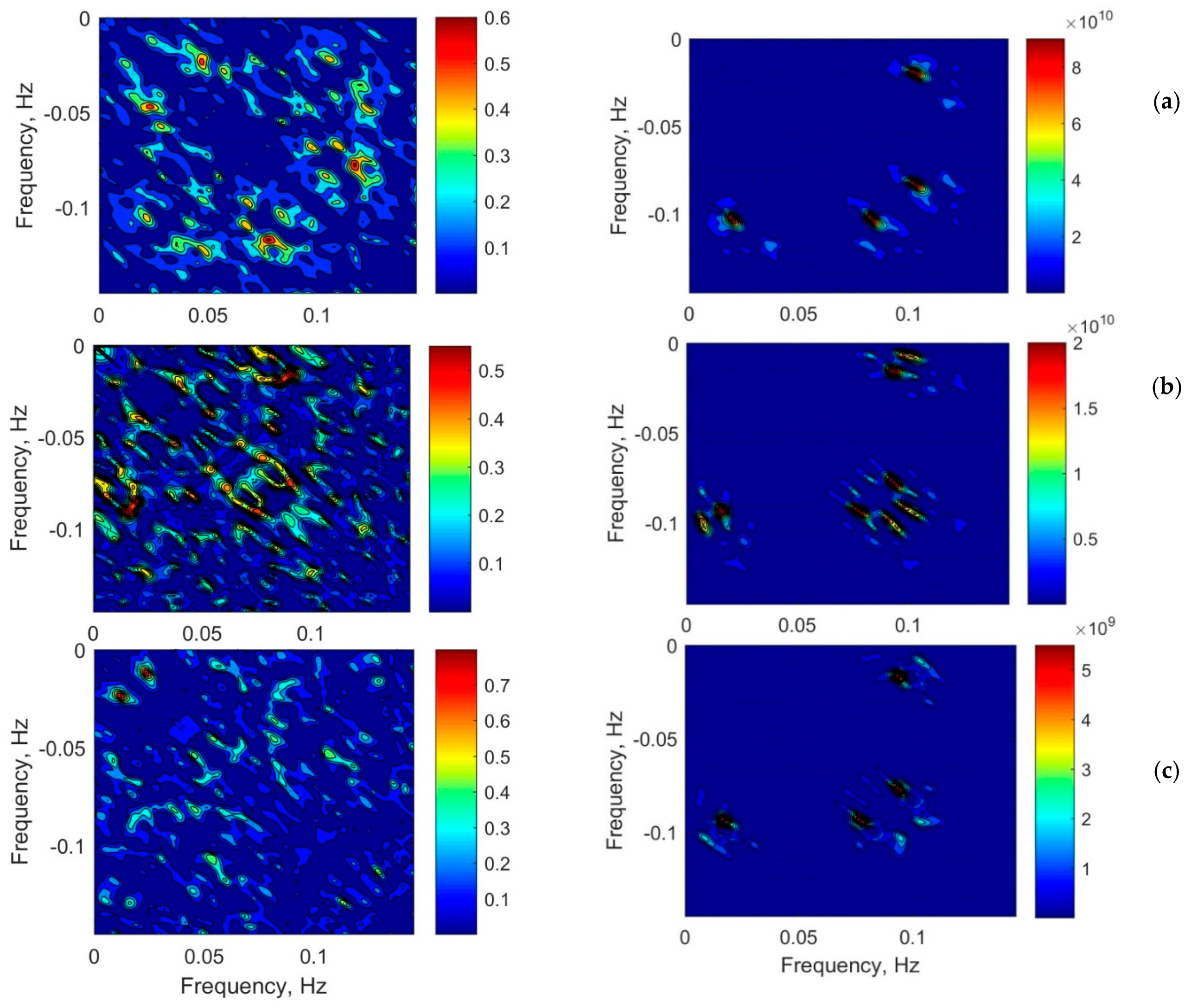
Figure 6 shows the results of bispectral analysis for waves propagating in water. The modules of the bispectrum demonstrate that the two areas of wave harmonics involved in the nonlinear interaction exist—the frequency in the vicinity of the main spectral peak (about 0.08–0.1 Hz) and the infragravity area of about 0.02–0.04 Hz. High values of bicoherence (2) of about 0.5 confirm that a new low-frequency peak at 0.08 Hz is formed as a result of the difference nonlinear interaction between frequencies of 0.02 Hz and the main peak frequency of 0.1 Hz. The peak at a frequency of 0.02 Hz can be interpreted as bound infragravity waves and it is the result of nonlinear interactions due to the natural width of the wave spectrum in the vicinity of its peak (for example, [
24]). The frequencies close to the main frequency of the initial peak 0.1 Hz are present in the formation of infragravity waves by difference wave interactions. Further, the frequency of 0.02 Hz due to the difference three wave interactions with the main peak frequency (0.1 Hz) forms a new low-frequency peak at 0.08 Hz. The peak at frequency 0.04 Hz is the result of the difference nonlinear interactions of frequencies at 0.08 and 0.12 Hz and 0.06 and 0.02 Hz. Moreover, the difference three wave interactions of the frequency 0.12 Hz with frequency 0.04 Hz contribute to the frequency 0.08 Hz (
Figure 6). Wave energy transfer to the frequency close to the peak due to three-wave interactions of the main peak and frequencies of the infragravity range are also observed in [
12].
As shown in [
25], the sign of the imaginary part of the bispectrum (1) shows the direction of the wave energy transfer. This can be additional confirmation of the origin of the peak at the frequency of 0.08 Hz due to difference nonlinear wave interactions.
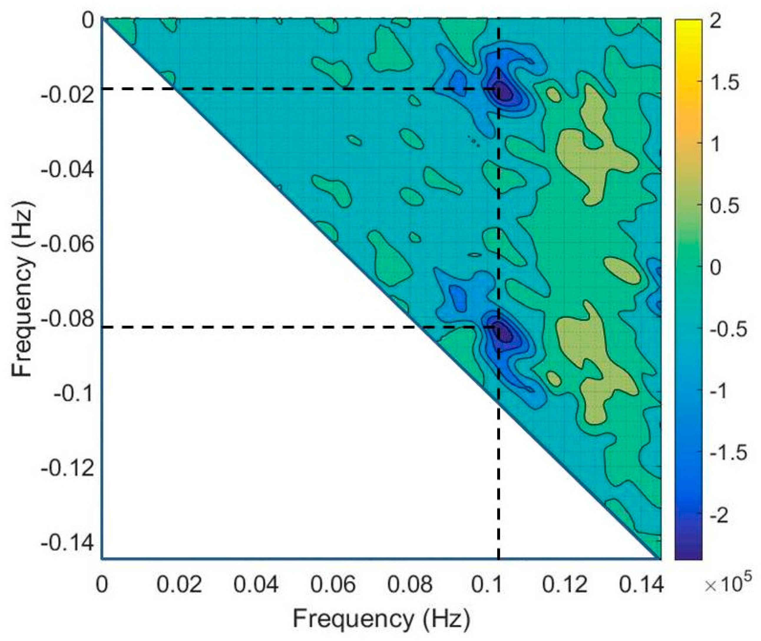
Figure 7 shows the imaginary part of the bispectrum for waves propagating in water at a distance of 500 m (the corresponding bispectra and the bicoherence function are shown in
Figure 6a). It is clearly seen that the frequencies 0.02 Hz and 0.08 Hz are in difference three-wave interactions with the frequency of 0.1 Hz (peak of the spectrum), since the imaginary part of the bispectrum has maximum negative values at these frequencies. Negative values of the imaginary part of the bispectrum at the considered frequencies are also observed at other distances (corresponding figures are not shown to save space in the article).
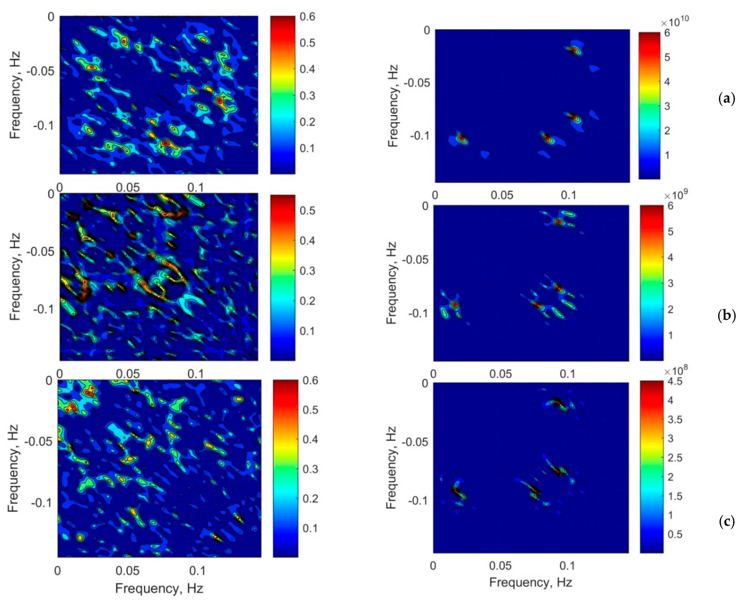
The results of the bispectral analysis for waves propagating over viscous mud are presented in
Figure 8. As in the case of propagation of waves in clear water, a low-frequency peak (0.08 Hz), which then shifts the frequency, is formed as a result of the difference interactions between the frequency of 0.02 Hz and the main frequency of 0.1 Hz. This is confirmed by the high values of the squared bicoherence function (2) (
Figure 8). It is clearly seen that
Figure 6 and
Figure 8 for the bicoherence function and bispectra are almost the same. The same is evident concerning the analysis of the imaginary part of the bispectrum (corresponding figures are not shown to save space in the article). Thus, we can conclude that for waves propagating over viscous mud, the nonlinear processes are the same as in water.
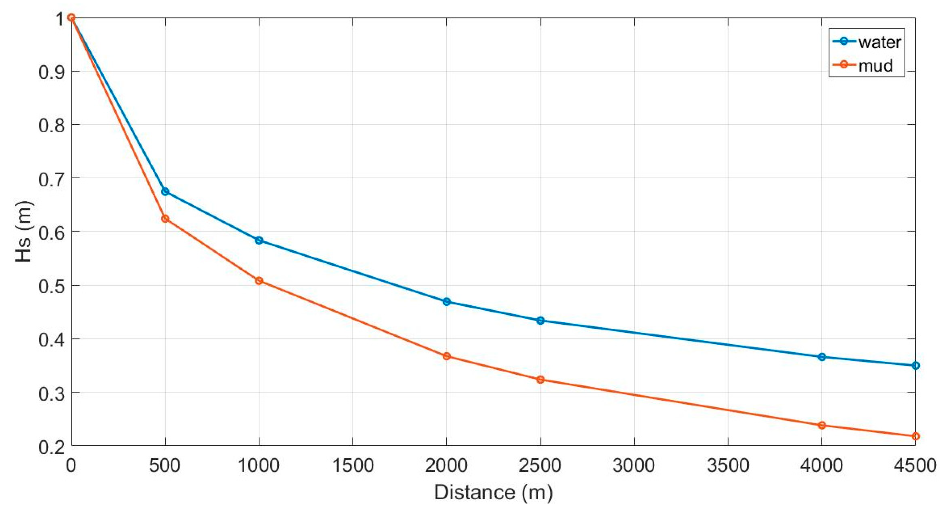
In general, the wave height significantly decreases, which indicates significant dissipative processes occurring both during the transformation of waves in shallow water and over mud (
Figure 9). It is visible that after 4500 m of wave propagation over mud, the wave height attenuation is two times more than in water. However, a reduction in significant wave height and the dissipation process occurs according to the same scenario: waves lose most of their height in the first 1000 m of the wave transformation corresponding to the formation of a new peak and then the reduction in wave height slows down.
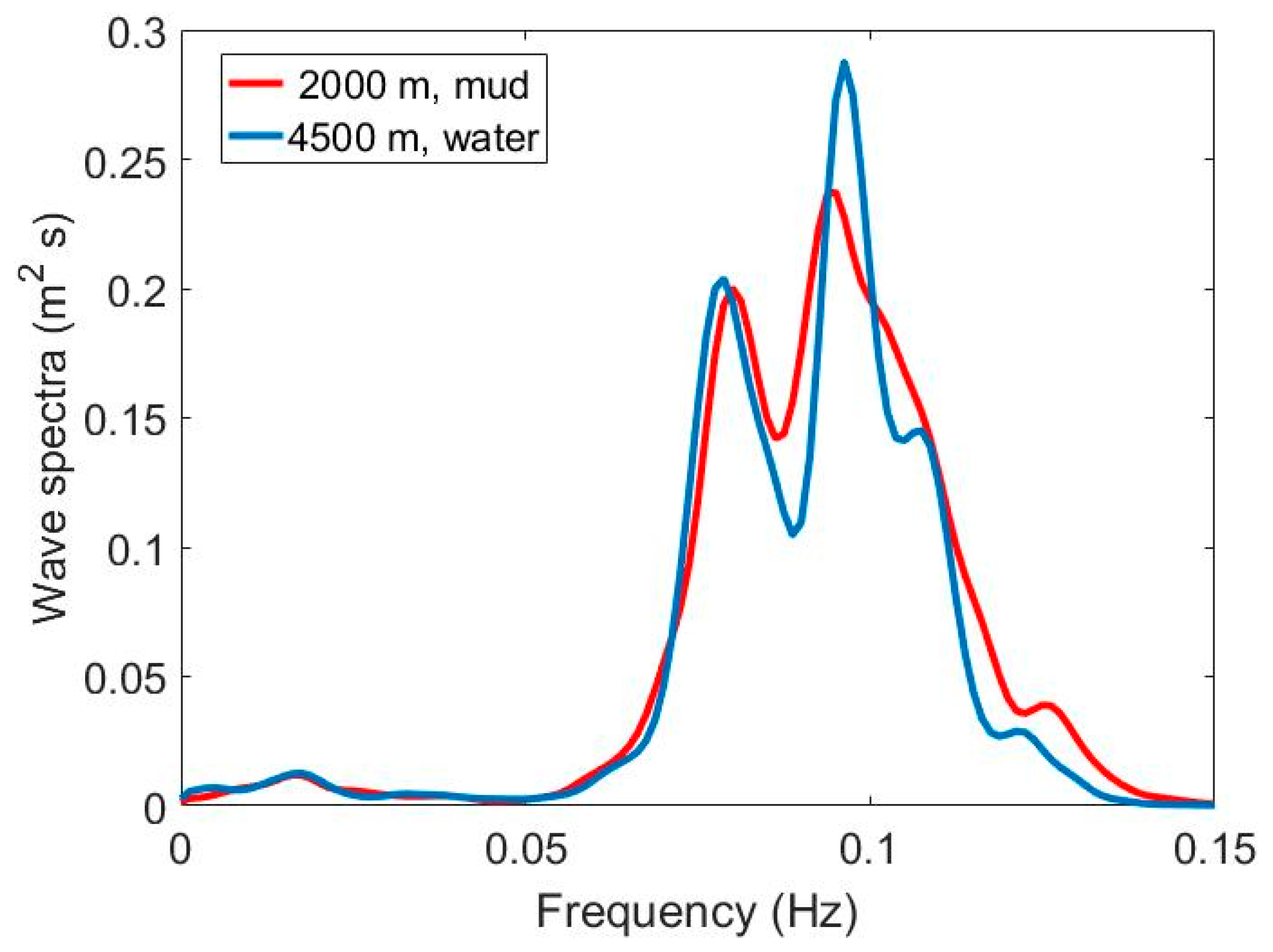
The dissipation processes and reduction in significant wave heights are stronger in viscous mud and this leads to the fact that the peak at a frequency of 0.08 Hz becomes dominant after 4000 m of wave propagation. Similarly, at the same distance in the spectrum of waves propagating in clear water, this peak also exists, but it is not the main one. The decrease in the main peak depends on the dissipation. The significant wave height of waves propagating in water at the distance of 4500 m will have practically the same height for the waves propagating over viscous mud at the distance of 2000 m. If we compare the shape of wave spectra in water and viscous mud at these distances (
Figure 10), we can find that the magnitude of the low-frequency peak (frequency 0.08 Hz) is the same regardless of the viscosity of the medium. It depends on the nonlinear processes occurring while propagating. However, the magnitude of the main peak for waves propagating in mud is significantly lower, which is associated with stronger dissipative processes. The low-frequency peak becomes dominant earlier due to the rapid reduction in the main peak due to the dissipation process. So, the dissipation accelerates frequency downshifting, thereby decreasing the energy of the wave spectrum in the frequency range of the main peak.
Let us consider qualitatively how the features of wave transformation and downshifting, which we observed, could have an impact on cohesive sediment transport and the formation of mudbanks. In [
26,
27], the cohesive transport model based on the wave attenuation coefficient was suggested. For waves propagating above the cohesive sediments bed, it was found that due to dissipation, the wave height changes according to the exponential law [
26,
27]
where
is the distance along the wave propagation positive towards the shore from the shore up to
—the initial point of the wave propagation in the sea,
is initial wave height at
and
k is the coefficient of wave height attenuation due to wave dissipation. The wave height attenuation coefficient
k characterizes the fluidization potential of the mud. It is a function of the rheology of the bed, incident wave height and, probably, the wave period [
26,
27].
Lee [
27] found an analytical solution for the bed profile and suggested that the erosive and accumulative types of profiles depend on the dimensionless wave attenuation coefficient
, where
is the distance from the initial seaward (
) and end shoreward points of the wave propagation. If
then the bed profile is accretive or convex upward. Alternatively, if
, it is erosive or concave. These assumptions and the analytically predicted bottom profile were successfully validated according to the data of laboratory and field experiments, including data presented in [
13] from the Kerala region [
27].
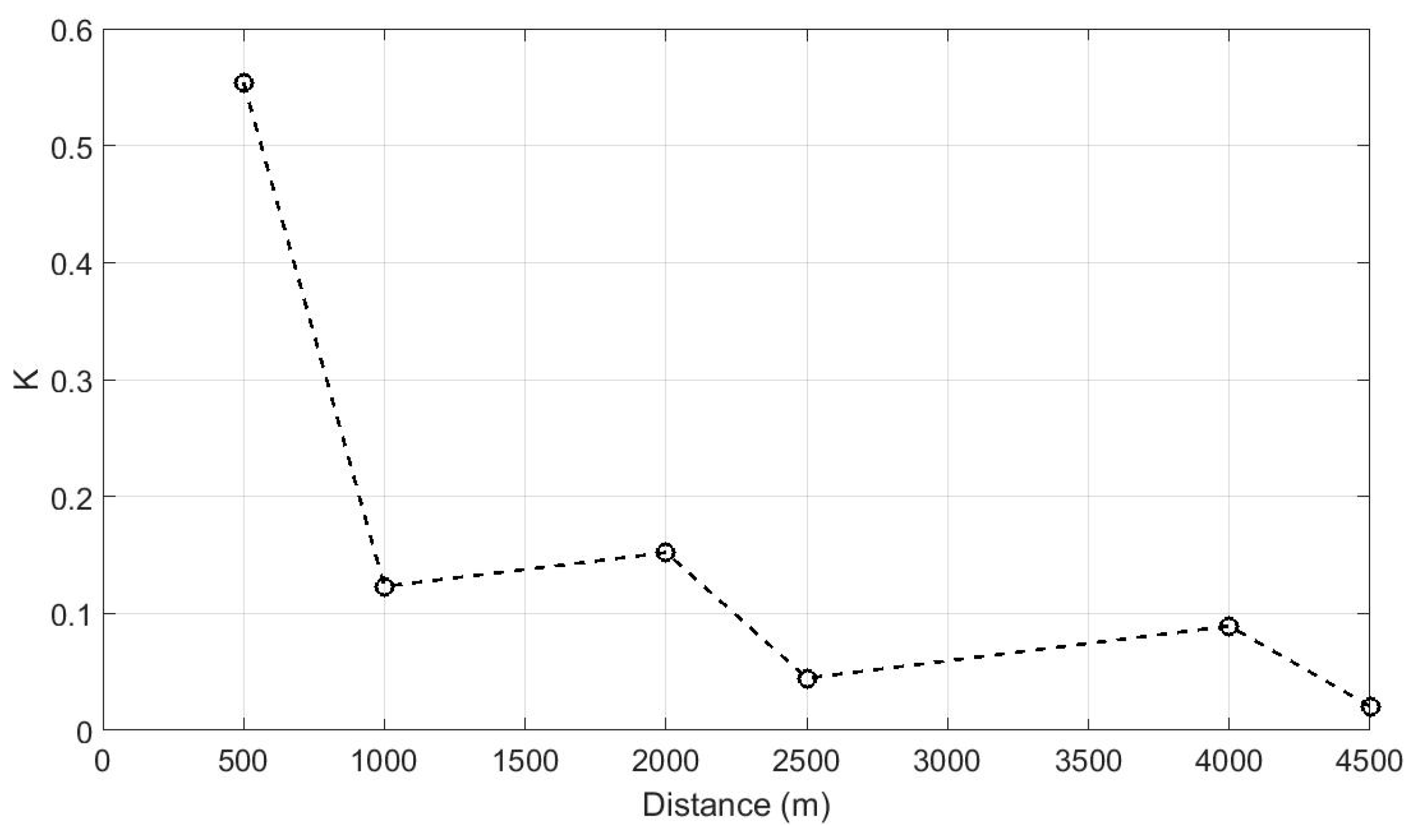
Based on the foregoing discussion, we calculated the coefficient
K for waves with a JONSWAP spectrum (peak enhancement parameter = 1,
m and
s) in different sections along the distance of the wave transformation over viscous mud (
Figure 11). At the distance of the first 500 m of wave transformation, the bed profile can be washed out and fluidization of the mud (
) will occur. Further, at distances of more than 2000 m, where a distinct new low-frequency peak of the spectrum is formed, the coefficient K decreases significantly and becomes less than 0.1, which will lead to the accumulation of sediments at these distances, i.e., formation of a mudbank. If we formally divide the profile into two sections of 0–2000 m, when a new low-frequency peak is formed, and 2500–4500 m, when a low-frequency peak exists and the frequency of the spectrum maximum downshifts, then these two sections differ significantly by the coefficient
(0.99 and 0.35, respectively). According to Lee’s model [
27], this leads to the presence of two completely different bottom profiles—erosional, characterizing increased dissipation of wave energy, and accumulative, characterizing a decrease in dissipation due to nonlinear transformation of waves and downshift of their frequency. Thus, nonlinear transformation of waves, accompanied by frequency downshifting, can be one of the possible mechanisms of the formation of a mudbank. Erosion (or cohesive sediments removal) will be in the area where an additional peak develops, and accumulation (mudbank formation) will be in the area where downshifting occurs. The proposed mechanism needs further verification based on more field or laboratory data.
4. Conclusions
The evolution of the spectrum of waves propagating in a constant water depth or over a flat bottom with a very low slope occurs with the formation of a characteristic spectrum having a low-frequency peak formed as a result of the difference nonlinear three-wave interactions between the main peak frequency and frequencies of the infragravity range arising due to the natural width of the initial spectrum. During wave propagation, the peak frequency of the spectrum shifts towards the low-frequency peak, i.e., downshifting occurs. Therefore, we find a low-frequency peak in the wave spectra off the Kerala coast, which is formed by nonlinear processes of wave transformations, and it is not swell waves as a result of the mixed sea state. Such a scenario of a changing wave spectrum is implemented independently of the viscosity of the medium. However, an increase in the viscosity and, accordingly, an increase in the influence of the dissipation process lead to the acceleration of frequency downshifting due to the rapid reduction in the wave energy in the main peak frequency.
It was observed that the nonlinear transformation of waves with frequency downshifting could be one of the possible wave mechanisms of mudbank formation. As the frequency downshifting process decreases, the wave attenuation, according to the cohesive sediments transport model [
27] based on the dimensionless wave attenuation coefficient, can lead to formation first, erosion and further formation of an accumulative muddy profile or mudbank. This suggested mechanism still has to be verified with more field or laboratory experiments to clarify the unidentified inferences on how wave transformation can influence mudbank formation.


