Sensitivity of Flood Hazard and Damage to Modelling Approaches


Abstract
:1. Introduction
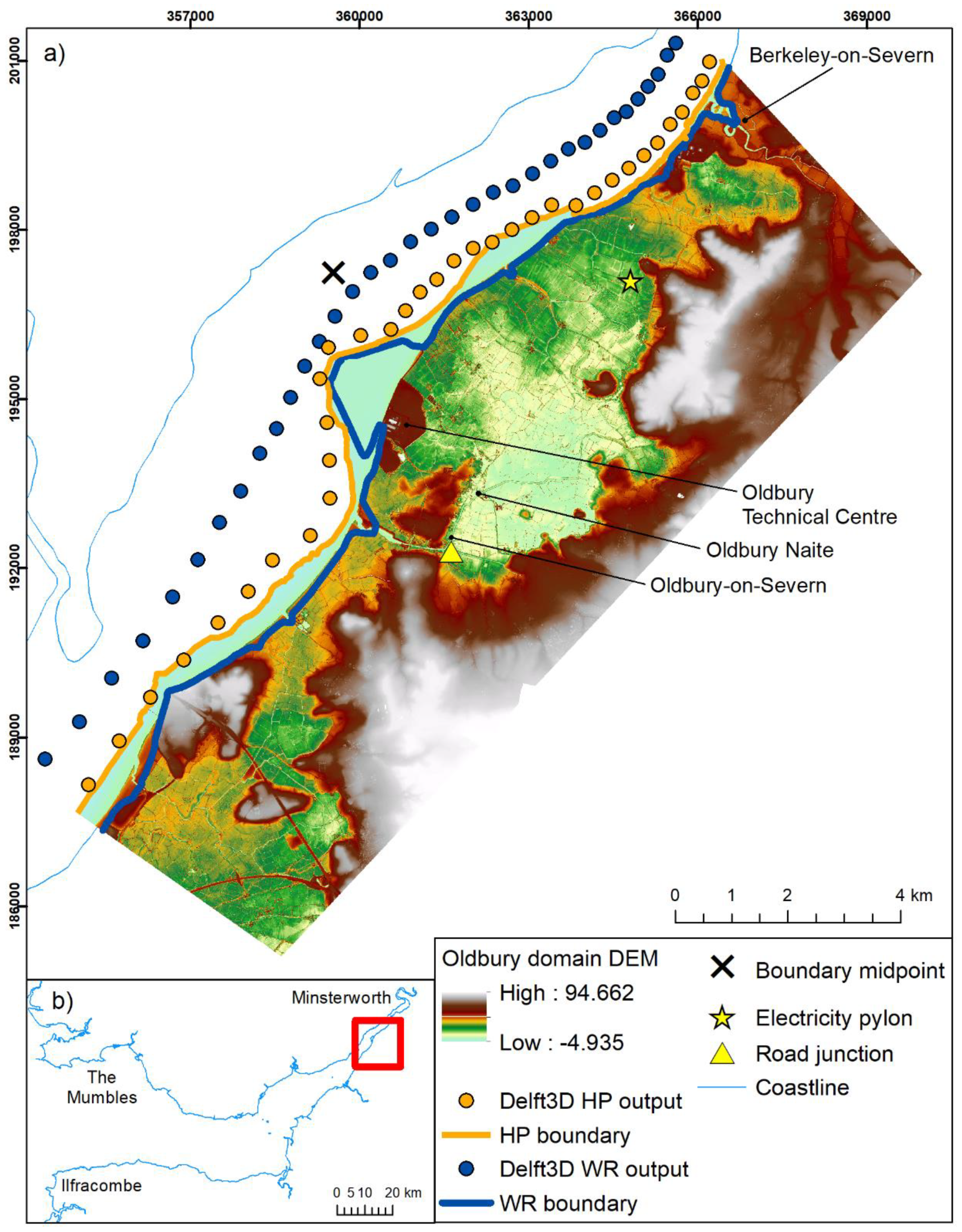
Case Study
2. Method
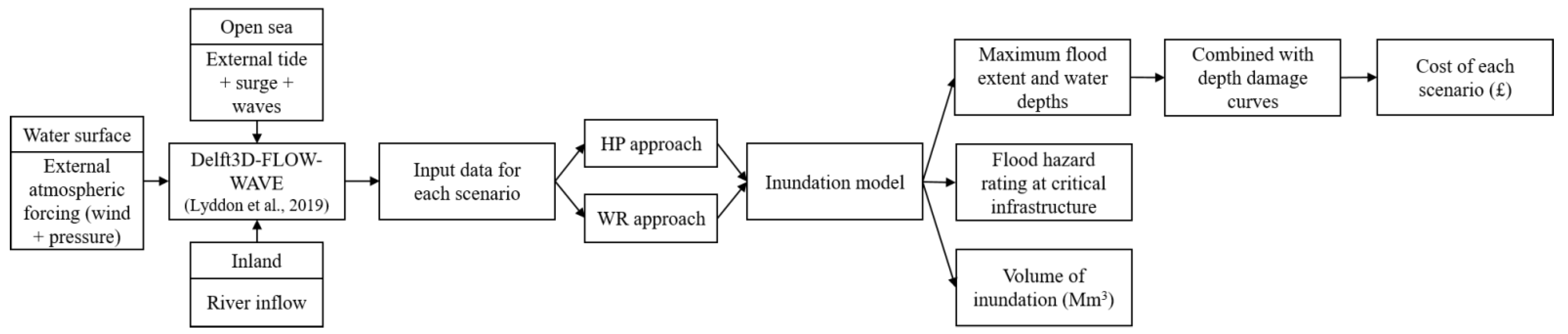
2.1. Inundation Model
2.2. Input Data
2.2.1. Historic Storm Events
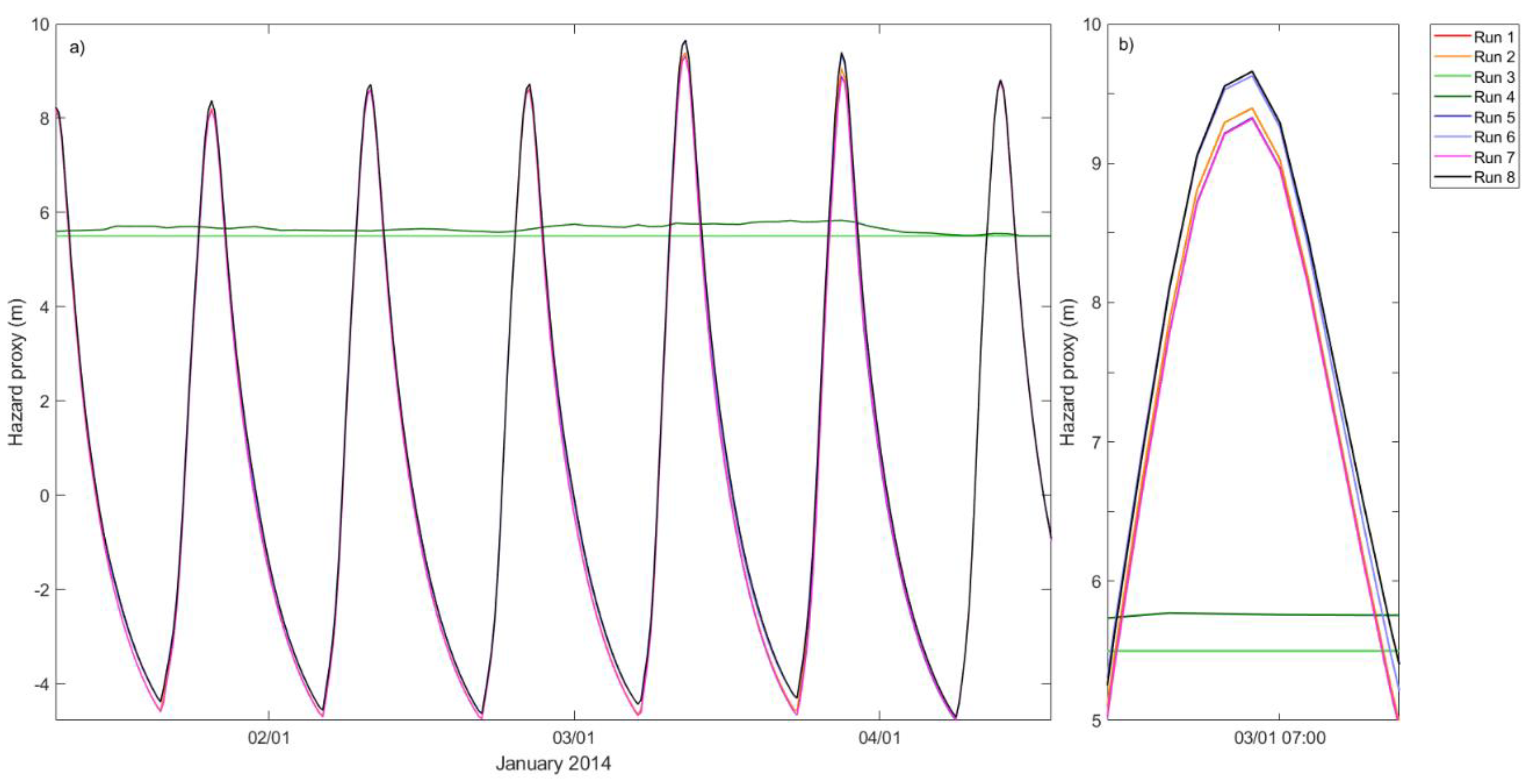
2.2.2. Coastal Hazard Uncertainty
2.3. Inundation Model Boundary Conditions
- Hazard proxy (HP = WL + ½ Hs) is calculated from Delft3D outputs and imposed at the low water mark, to resolve wetting and drying in the inundation model.
- WL and Hs from further offshore are used to calculate wave runup using Stockdon formula [59], and provide runup level at the crest.
2.3.1. Hazard Proxy Approach
2.3.2. Wave Runup Approach
2.4. Model Validation and Calibration
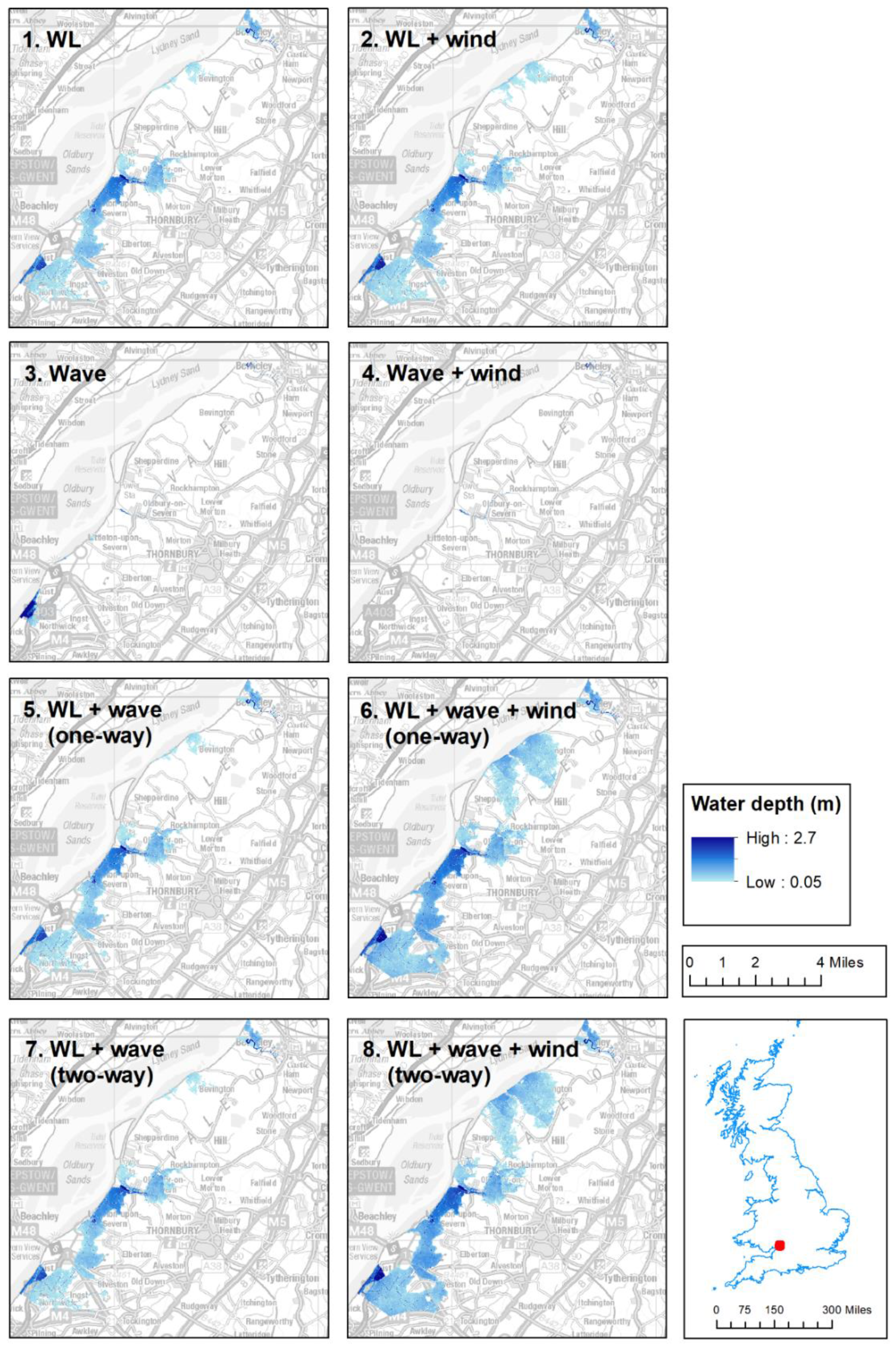
2.5. Flood Inundation Scenarios
2.6. Depth Damage Curves
3. Results
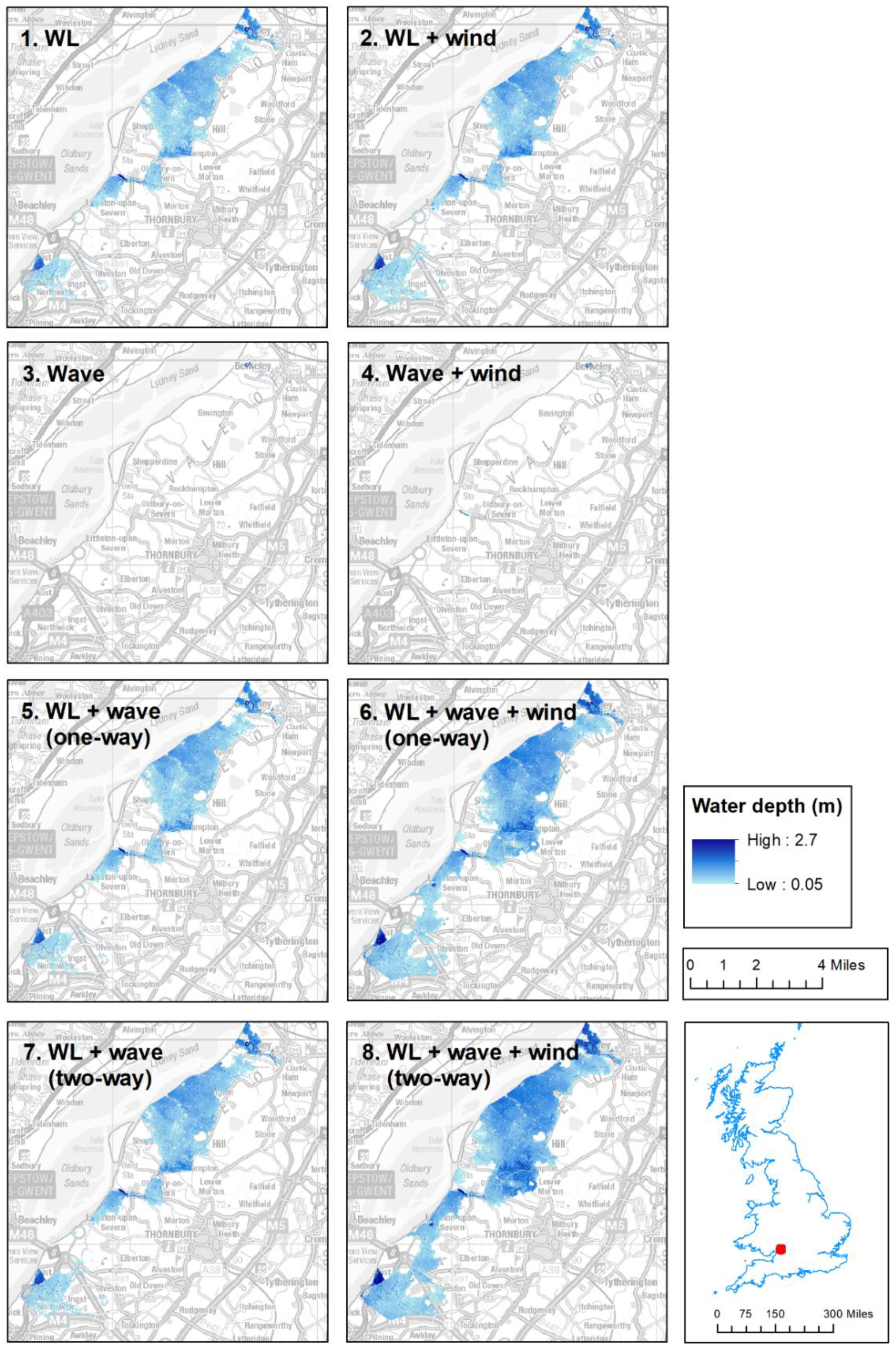
3.1. Depth and Extent of Inundation
3.1.1. January 14 Hazard Proxy (HP)
3.1.2. January 14 Wave Runup (WR)
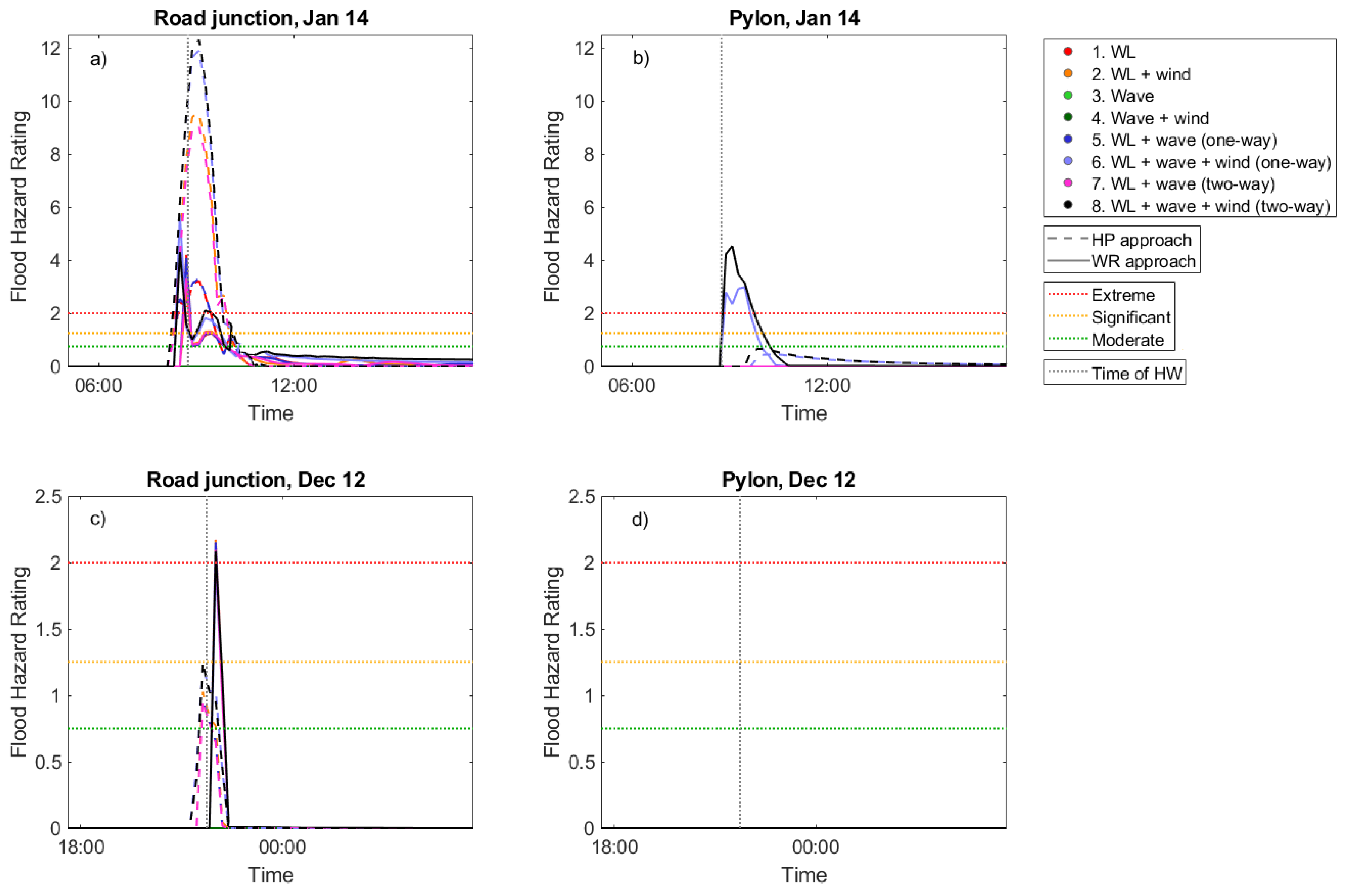
3.2. Flood Hazard Rating at Operational Sites
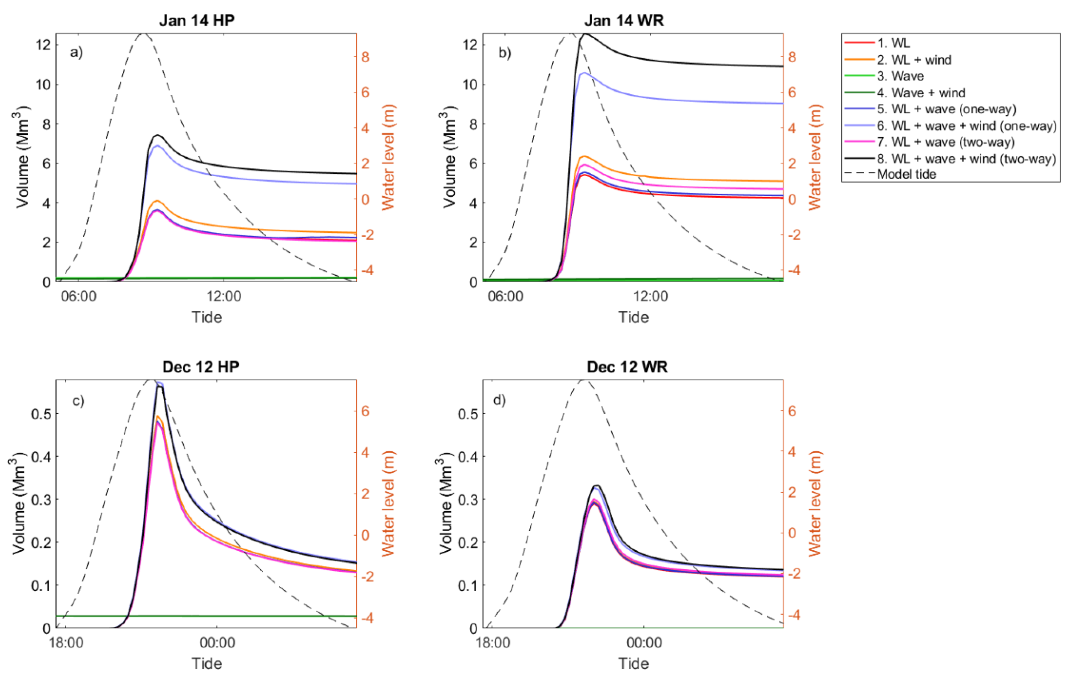
3.3. Volume of Inundation in the Model Domain
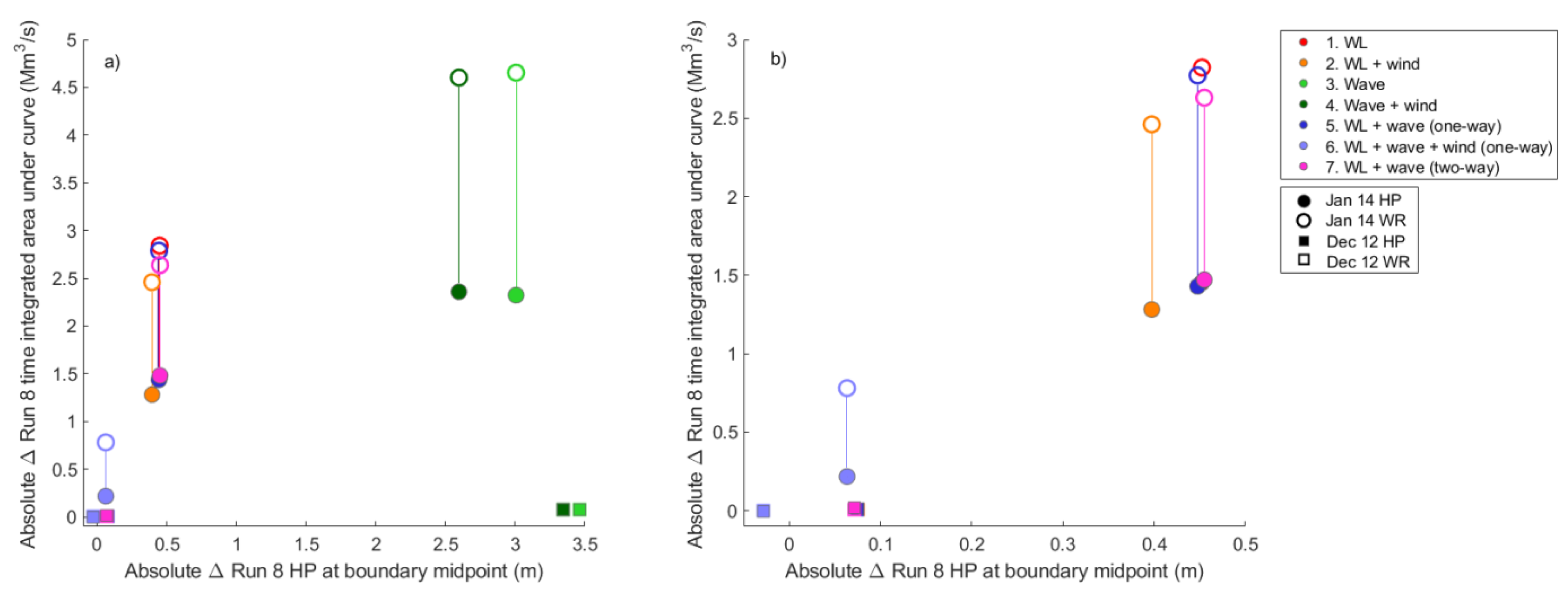
3.4. Flood Hazard Sensitivity to Coastal Hazard Uncertainty
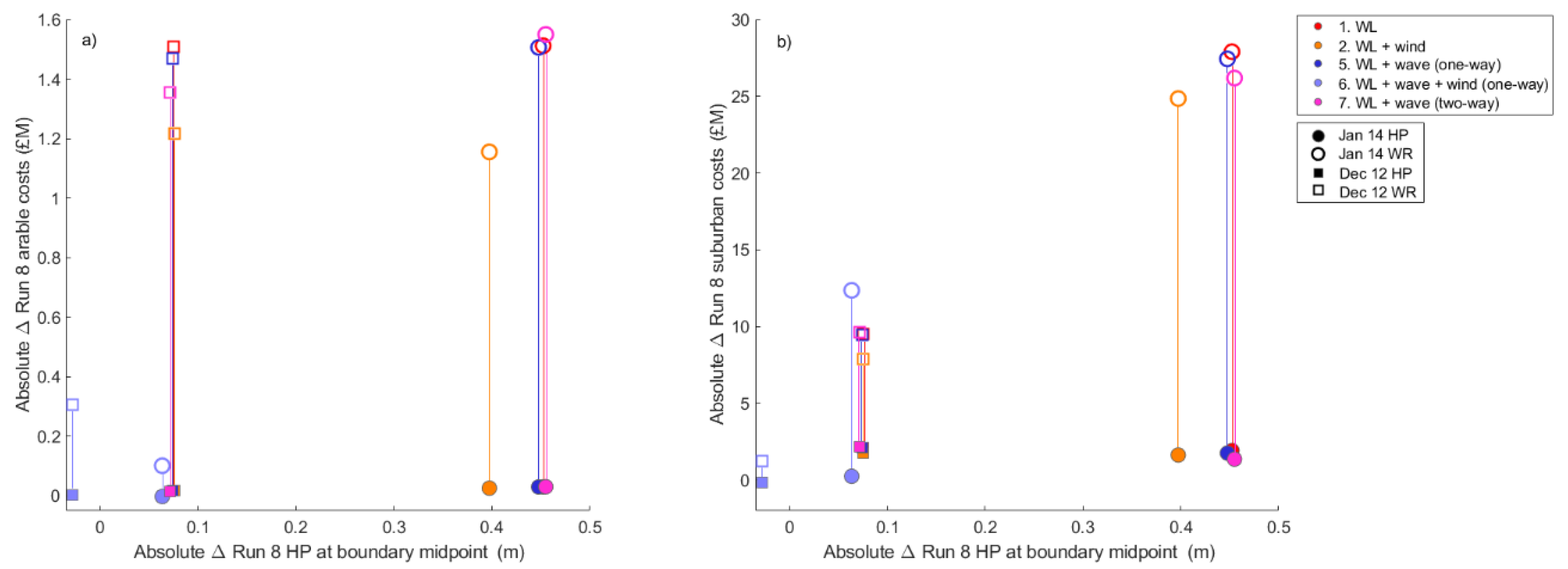
3.5. Economic Cost of Inundation for Arable and Suburban Land Uses
4. Discussion
4.1. Flood Hazard Sensitivity to Coastal Hazard Conditions and Approach to Forcing the Model Boundary
4.1.1. Influence of Coastal Hazard Condition
4.1.2. Influence of Approach to Forcing the Model Boundary
4.2. Flood Hazard Sensitivity in Coastal Zones Worldwide
4.3. Implications for Inundation under Future Sea-Level Scenarios
4.4. Limitations
5. Conclusions
Supplementary Materials
Author Contributions
Funding
Acknowledgments
Conflicts of Interest
References
- Adikari, Y.; Osti, R.; Noro, T. Flood-related disaster vulnerability: An impending crisis of megacities in Asia. J. Flood Risk Manag. 2010, 3, 185–191. [Google Scholar] [CrossRef]
- Sekovski, I.; Newton, A.; Dennison, W.C. Megacities in the coastal zone: Using a driver-pressure-state-impact-response framework to address complex environmental problems. Estuar. Coast. Shelf Sci. 2012, 96, 48–59. [Google Scholar] [CrossRef]
- Chen, R.; Zhang, Y.; Xu, D.; Liu, M. Climate change and coastal megacities: Disaster risk assessment and responses in Shanghai City. In Climate Change, Extreme Events and Disaster Risk Reduction; Springer Science and Business Media LLC: Berlin, Germany, 2017; pp. 203–216. [Google Scholar]
- Hendry, A.; Haigh, I.D.; Nicholls, R.J.; Winter, H.; Neal, R.; Wahl, T.; Joly-Laugel, A.; Darby, S.E. Assessing the characteristics and drivers of compound flooding events around the UK coast. Hydrol. Earth Syst. Sci. 2019, 23, 3117–3139. [Google Scholar] [CrossRef] [Green Version]
- Lyddon, C.; Brown, J.M.; Leonardi, N.; Plater, A.J. Flood hazard assessment for a hyper-tidal estuary as a function of tide-surge-morphology interaction. Chesap. Sci. 2018, 41, 1565–1586. [Google Scholar] [CrossRef] [Green Version]
- Narayan, S.; Hanson, S.; Nicholls, R.J.; Clarke, D.; Willems, P.; Ntegeka, V.; Monbaliu, J. A holistic model for coastal flooding using system diagrams and the Source-Pathway-Receptor (SPR) concept. Nat. Hazards Earth Syst. Sci. 2012, 12, 1431–1439. [Google Scholar] [CrossRef] [Green Version]
- Desplanque, C.; Mossman, D.J. Storm tides of the Fundy. Geogr. Rev. 1999, 89, 23–33. [Google Scholar] [CrossRef]
- Greenberg, D.; Blanchard, W.; Smith, B.; Barrow, E. Climate change, mean sea level and high tides in the bay of Fundy. Atmos. Ocean. 2012, 50, 261–276. [Google Scholar] [CrossRef]
- Muchan, K.; Lewis, M.; Hannaford, J.; Parry, S. The winter storms of 2013/2014 in the UK: Hydrological responses and impacts. Weather 2015, 70, 55–61. [Google Scholar] [CrossRef] [Green Version]
- Sibley, A.; Cox, D.; Titley, H. Coastal flooding in England and Wales from Atlantic and North Sea storms during the 2013/2014 winter. Weather 2015, 70, 62–70. [Google Scholar] [CrossRef]
- Yang, J.; Li, L.; Zhao, K.; Wang, P.; Wang, D.; Sou, I.M.; Yang, Z.; Hu, J.; Tang, X.; Mok, K.M.; et al. A comparative study of typhoon Hato (2017) and typhoon Mangkhut (2018)—Their Impacts on coastal inundation in Macau. J. Geophys. Res. Ocean. 2019, 124, 9590–9619. [Google Scholar] [CrossRef]
- Haigh, I.D.; Wadey, M.P.; Wahl, T.; Ozsoy, O.; Nicholls, R.J.; Brown, J.M.; Horsburgh, K.; Gouldby, B. Spatial and temporal analysis of extreme sea level and storm surge events around the coastline of the UK. Sci. Data 2016, 3, 160107. [Google Scholar] [CrossRef] [PubMed] [Green Version]
- Del Río, L.; Plomaritis, T.; Benavente, J.; Valladares, M.; Ribera, P.; González, J.B. Establishing storm thresholds for the Spanish Gulf of Cádiz coast. Geomorphology 2012, 144, 13–23. [Google Scholar] [CrossRef]
- Teng, J.; Jakeman, A.; Vaze, J.; Croke, B.; Dutta, D.; Kim, S. Flood inundation modelling: A review of methods, recent advances and uncertainty analysis. Env. Model. Softw. 2017, 90, 201–216. [Google Scholar] [CrossRef]
- Sénéchal, N.; Coco, G.; Bryan, K.R.; Holman, R.A. Wave runup during extreme storm conditions. J. Geophys. Res. Space Phys. 2011, 116, 7. [Google Scholar] [CrossRef] [Green Version]
- Suanez, S.; Cancouët, R.; Floc’H, F.; Blaise, E.; Ardhuin, F.; Filipot, J.-F.; Cariolet, J.-M.; Delacourt, C. Observations and predictions of wave runup, extreme water levels, and medium-term dune erosion during storm conditions. J. Mar. Sci. Eng. 2015, 3, 674–698. [Google Scholar] [CrossRef] [Green Version]
- EurOtop. Manual on Wave Overtopping of Sea Defences and Related Structures, 2nd ed.; Boyens Medien GmbH: Heide, Germany, 2018. [Google Scholar]
- Knight, P.J.; Prime, T.; Brown, J.M.; Morrissey, K.; Plater, A.J. Application of flood risk modelling in a web-based geospatial decision support tool for coastal adaptation to climate change. Nat. Hazards Earth Syst. Sci. 2015, 15, 1457–1471. [Google Scholar] [CrossRef] [Green Version]
- Prime, T.; Brown, J.M.; Plater, A.J. Physical and economic impacts of sea-level rise and low probability flooding events on coastal communities. PLoS ONE 2015, 10, e0117030. [Google Scholar] [CrossRef] [Green Version]
- Didier, D.; Baudry, J.; Bernatchez, P.; Dumont, D.; Sadegh, M.; Bismuth, E.; Bandet, M.; Dugas, S.; Sévigny, C. Multihazard simulation for coastal flood mapping: Bathtub versus numerical modelling in an open estuary, Eastern Canada. J. Flood Risk Manag. 2018, 12, e12505. [Google Scholar] [CrossRef]
- Thompson, D.A.; Karunarathna, H.U.; Reeve, D.E. Modelling extreme wave overtopping at aberystwyth promenade. Water 2017, 9, 663. [Google Scholar] [CrossRef] [Green Version]
- Karunarathna, H.U.; Brown, J.M.; Chatzirodou, A.; Dissanayake, P.; Wisse, P. Multi-timescale morphological modelling of a dune-fronted sandy beach. Coast. Eng. 2018, 136, 161–171. [Google Scholar] [CrossRef]
- Vitousek, S.; Barnard, P.; Fletcher, C.H.; Frazer, L.N.; Erikson, L.; Storlazzi, C.D. Doubling of coastal flooding frequency within decades due to sea-level rise. Sci. Rep. 2017, 7, 1399. [Google Scholar] [CrossRef] [PubMed]
- DEFRA. Flood Risks to People (Phase 2). Flood Risks to People Phase 2 FD2321 Tech Rep 1 [Internet]. 2003; p. 117. Available online: http://randd.defra.gov.uk/Document.aspx?Document=FD2317_1060_TRP.pdf (accessed on 22 January 2020).
- Amante, C. Estimating coastal digital elevation model uncertainty. J. Coast. Res. 2018, 34, 1382–1397. [Google Scholar] [CrossRef] [Green Version]
- Lyddon, C.E.; Brown, J.M.; Leonardi, N.; Saulter, A. Quantification of the uncertainty in coastal storm hazard predictions due to wave—Current interaction and wind forcing. Geophys Res Lett. 2019, 46, 14576–14585. [Google Scholar] [CrossRef] [Green Version]
- Stephens, S.A.; Bell, R.; Lawrence, J. Applying principles of uncertainty within coastal hazard assessments to better support coastal adaptation. J. Mar. Sci. Eng. 2017, 5, 40. [Google Scholar] [CrossRef]
- Sayers, P.; Gouldby, B.; Simm, J.; Meadowcroft, I.; Hall, J. Risk, performance and uncertainty in flood and coastal defence—A review. R&D Tech. Rep. 2003, 115, 6–27. [Google Scholar]
- Hewston, R.; Zou, Q.; Reeve, D.; Pan, S.; Chen, Y. Quantifying uncertainty in tide, surge and wave modelling during extreme storms. In Proceedings of the BHS 3rd International Symposium, Managing Consequences of Changing Global Environment, British Hydrological Society, Newcastle University, Newcastle, UK, 19–23 July 2010. [Google Scholar]
- Kumbier, K.; Carvalho, R.C.; Vafeidis, A.T.; Woodroffe, C.D. Investigating compound flooding in an estuary using hydrodynamic modelling: A case study from the Shoalhaven River, Australia. Nat. Hazards Earth Syst. Sci. 2018, 18, 463–477. [Google Scholar] [CrossRef] [Green Version]
- Savage, J.T.S.; Pianosi, F.; Bates, P.D.; Freer, J.E.; Wagener, T. Quantifying the importance of spatial resolution and other factors through global sensitivity analysis of a flood inundation model. Water Resour. Res. 2016, 52, 9146–9163. [Google Scholar] [CrossRef]
- Purvis, M.J.; Bates, P.D.; Hayes, C.M. A probabilistic methodology to estimate future coastal flood risk due to sea level rise. Coast. Eng. 2008, 55, 1062–1073. [Google Scholar] [CrossRef]
- Quinn, N.; Bates, P.D.; Siddall, M. The contribution to future flood risk in the Severn Estuary from extreme sea level rise due to ice sheet mass loss. J. Geophys. Res. Ocean. 2013, 118, 5887–5898. [Google Scholar] [CrossRef]
- Lewis, M.J.; Schumann, G.J.-P.; Bates, P.D.; Horsburgh, K. Understanding the variability of an extreme storm tide along a coastline. Estuar. Coast. Shelf Sci. 2013, 123, 19–25. [Google Scholar] [CrossRef]
- Pianosi, F.; Beven, K.; Freer, J.E.; Hall, J.W.; Rougier, J.; Stephenson, D.; Wagener, T. Sensitivity analysis of environmental models: A systematic review with practical workflow. Env. Model. Softw. 2016, 79, 214–232. [Google Scholar] [CrossRef]
- Pasquier, U.; He, Y.; Hooton, S.; Goulden, M.; Hiscock, K.M. An integrated 1D–2D hydraulic modelling approach to assess the sensitivity of a coastal region to compound flooding hazard under climate change. Nat. Hazards 2018, 98, 915–937. [Google Scholar] [CrossRef] [Green Version]
- Sanuy, M.; Jimenez, J.A.; Ortego, M.I.; Toimil, A. Differences in assigning probabilities to coastal inundation hazard estimators: Event versus response approaches. J. Flood Risk Manag. 2019, 13, 7. [Google Scholar] [CrossRef] [Green Version]
- Hall, J.W.; Solomatine, D. A framework for uncertainty analysis in flood risk management decisions. Int. J. River Basin Manag. 2008, 6, 85–98. [Google Scholar] [CrossRef] [Green Version]
- SurgeWatch. An Interactive Database of UK Coastal Flooding [Internet]. 2018. Available online: https://www.surgewatch.org/ (accessed on 11 July 2020).
- Haigh, I.D.; Wadey, M.P.; Gallop, S.L.; Loehr, H.; Nicholls, R.J.; Horsburgh, K.; Brown, J.M.; Bradshaw, E. A user-friendly database of coastal flooding in the United Kingdom from 1915–2014. Sci. Data 2015, 2, 150021. [Google Scholar] [CrossRef]
- Uncles, R. Physical properties and processes in the Bristol Channel and Severn Estuary. Mar. Pollut. Bull. 2010, 61, 5–20. Available online: http://linkinghub.elsevier.com/retrieve/pii/S0025326X09005128 (accessed on 21 January 2020). [CrossRef]
- Pye, K.; Blott, S.J. A consideration of “extreme events” at Hinkley Point. Tech. Rep. Ser. 2010, 2010, 109. [Google Scholar]
- JBA. South Gloucestershire Council Strategic Flood Risk Assessment Level 2 for Oldbury on Severn JBA Project Manager. 2017. Available online: https://beta.southglos.gov.uk/wp-content/uploads/South-Gloucestershire-Council-level-2-Strategic-Flood-Risk-Assessment-SFRA-for-Oldbury-on-Severn-Sept-2017.pdf (accessed on 10 July 2020).
- South Gloucestershire Council. Southampton Local Flood Risk Management Strategy Summary [Internet]. 2014. Available online: https://www.southampton.gov.uk/policies/Southampton LFRMS Main Report – Final - October 2014.pdf (accessed on 10 July 2020).
- Office for National Statistics. Oldbury, Berkeley and Thornbury parish [Internet]. 2011. Available online: https://www.nomisweb.co.uk/ (accessed on 20 April 2020).
- Bates, P.D.; Dawson, R.J.; Hall, J.W.; Horritt, M.S.; Nicholls, R.J.; Wicks, J.; Hassan, M.A.A.M. Simplified two-dimensional numerical modelling of coastal flooding and example applications. Coast. Eng. 2005, 52, 793–810. [Google Scholar] [CrossRef]
- Wadey, M.P.; Nicholls, R.J.; Hutton, C. Coastal flooding in the solent: An integrated analysis of defences and inundation. Water 2012, 4, 430–459. [Google Scholar] [CrossRef] [Green Version]
- Skinner, C.; Coulthard, T.J.; Parsons, D.R.; Ramirez, J.; Mullen, L.; Manson, S. Simulating tidal and storm surge hydraulics with a simple 2D inertia based model, in the Humber Estuary, U.K. Estuar. Coast. Shelf Sci. 2015, 155, 126–136. [Google Scholar] [CrossRef]
- Smith, R.A.; Bates, P.D.; Hayes, C. Evaluation of a coastal flood inundation model using hard and soft data. Env. Model. Softw. 2011, 30, 35–46. [Google Scholar] [CrossRef]
- Quinn, N.; Lewis, M.; Wadey, M.P.; Haigh, I.D. Assessing the temporal variability in extreme storm-tide time series for coastal flood risk assessment. J. Geophys. Res. Ocean. 2014, 119, 4983–4998. [Google Scholar] [CrossRef]
- Environment Agency Geomatics. LiDAR Download [Internet]. Available online: https://www.arcgis.com/apps/MapJournal/index.html?appid=c6cef6cc642a48838d38e722ea8ccfee (accessed on 12 August 2019).
- Seenath, A. Effects of DEM resolution on modeling coastal flood vulnerability. Mar. Geod. 2018, 41, 581–604. [Google Scholar] [CrossRef] [Green Version]
- Md Ali, A.; Solomatine, D.P.; Di Baldassarre, G. Assessing the impact of different sources of topographic data on 1-D hydraulic modelling of floods. Hydrol. Earth Syst. Sci. 2015, 19, 631–643. [Google Scholar] [CrossRef] [Green Version]
- Karamouz, M.; Fereshtehpour, M. Modeling DEM errors in coastal flood inundation and damages: A spatial nonstationary approach. Water Resour. Res. 2019, 55, 6606–6624. [Google Scholar] [CrossRef]
- Saulter, A.; Bunney, C.; Li, J. Application of a Refined Grid Global Model for Operational Wave Forecasting; Met Office: Exeter, UK, 2016. [Google Scholar]
- Siddorn, J.; Good, S.A.; Harris, C.M.; Lewis, H.W.; Maksymczuk, J.; Martin, M.J.; Saulter, A. Research priorities in support of ocean monitoring and forecasting at the Met Office. Ocean Sci. 2016, 12, 217–231. [Google Scholar] [CrossRef] [Green Version]
- Walters, D.N.; Williams, K.D.; Boutle, I.A.; Bushell, A.C.; Edwards, J.; Field, P.R.; Lock, A.P.; Morcrette, C.J.; Stratton, R.A.; Wilkinson, J.; et al. The Met Office unified Model Global Atmosphere 4.0 and JULES Global Land 4.0 configurations. Geosci. Model. Dev. 2014, 7, 361–386. [Google Scholar] [CrossRef] [Green Version]
- Williams, J.A.; Horsburgh, K.J.; Evaluation and comparison of the operational Bristol Channel Model storm surge suite. NOC Res. Consult. Rep. 2013. Available online: http://nora.nerc.ac.uk/id/eprint/502138/1/NOC_R%26C_38.pdf (accessed on 21 January 2020).
- Stockdon, H.F.; Holman, R.A.; Howd, P.A.; Sallenger, A.H. Empirical parameterization of setup, swash, and runup. Coast. Eng. 2006, 53, 573–588. [Google Scholar] [CrossRef]
- Melby, J.; Nadal-Caraballo, N.; Kobayashi, N. Wave runup prediction for flood mapping. In Proceedings of the Coastal Engineering Proceedings; Coastal Engineering Research Council, Santander, Spain, 1–6 July 2012; Volume 1, pp. 1–15. [Google Scholar]
- Severn Estuary Coastal Group. Severn Estuary Shoreline Management Plan: PART B – POLICY STATEMENTS [Internet]. 2016. Available online: https://www.slideshare.net/SevernEstuary1/smp2-part-b-policy-statements-intro-sectionsfinal (accessed on 11 July 2020).
- Environment Agency. Flood Map for Planning [Internet]. 2020. Available online: https://flood-map-for-planning.service.gov.uk (accessed on 11 July 2020).
- Environment Agency. Managing Flood Risk on the Severn Estuary [Internet]. 2011. Available online: http://severnriverstrust.com/Managing Flood Risk on the Severn Estuary - Sth Gloucs Hinkley Point Somerset (Jan 11).pdf (accessed on 11 July 2020).
- Chow, V.T. Open-Channel Hydraulics; McGraw-Hill: New York, NY, USA, 1959; p. 680. [Google Scholar]
- Ding, Y.; Jia, Y.; Wang, S.S.Y. Identification of manning’s roughness coefficients in shallow water flows. J. Hydraul. Eng. 2004, 130, 501–510. [Google Scholar] [CrossRef] [Green Version]
- Lewis, M.J.; Horsburgh, K.; Bates, P.D.; Smith, R. Quantifying the uncertainty in future coastal flood risk estimates for the U.K. J. Coast. Res. 2011, 276, 870–881. [Google Scholar] [CrossRef]
- Brown, J.M.; Prime, T.; Phelps, J.J.; Barkwith, A.; Hurst, M.D.; Ellis, M.A.; Masselink, G.; Plater, A.J. Spatio-temporal variability in the tipping points of a coastal defense. J. Coast. Res. 2016, 75, 1042–1046. [Google Scholar] [CrossRef]
- Lewis, M.J.; Bates, P.D.; Horsburgh, K.; Neal, J.; Schumann, G.J.-P.; Neal, J.C. A storm surge inundation model of the northern Bay of Bengal using publicly available data. Q. J. R. Meteorol. Soc. 2013, 139, 358–369. [Google Scholar] [CrossRef]
- Bates, P.; Trigg, M.; Neal, J.; Dabrowa, A. LISFLOOD-FP User Manual: Code Release 5.9.6; University of Bristol: Bristol, UK, 2013. [Google Scholar]
- Penning-Rowsell, E.; Priest, S.; Parker, D.; Morris, J. Flood and Coastal Erosion Risk Management; Informa UK Limited: Colchester, UK, 2014. [Google Scholar]
- Rowland, C.S.; Morton, R.D.; Carrasco, L.; McShane, G.; O’Neil, A.W.; Wood, C.M. Land Cover Map 2015 (25m raster, GB) [Internet]. NERC Environmental Information Data Centre. 2017. Available online: https://doi.org/10.5285/bb15e200-9349-403c-bda9-b430093807c7 (accessed on 12 August 2019).
- Lewis, M.J.; Palmer, T.; Hashemi, R.; Robins, P.; Saulter, A.; Brown, J.; Lewis, H.; Neill, S. Wave-tide interaction modulates nearshore wave height. Ocean. Dyn. 2019, 69, 367–384. [Google Scholar] [CrossRef] [Green Version]
- Gallien, T.W.; Kalligeris, N.; Delisle, M.-P.; Tang, B.-X.; Lucey, J.T.D.; Winters, M.A. Coastal flood modeling challenges in defended urban backshores. Geoscience 2018, 8, 450. [Google Scholar] [CrossRef] [Green Version]
- Gallien, T.; Sanders, B.; Flick, R. Urban coastal flood prediction: Integrating wave overtopping, flood defenses and drainage. Coast. Eng. 2014, 91, 18–28. [Google Scholar] [CrossRef]
- Wahl, T.; Jain, S.; Bender, J.; Meyers, S.D.; Luther, M.E. Increasing risk of compound flooding from storm surge and rainfall for major US cities. Nat. Clim. Chang. 2015, 5, 1093–1097. [Google Scholar] [CrossRef]
- Hawkes, P.J.; Gouldby, B.P.; Tawn, J.A.; Owen, M.W. The joint probability of waves and water levels in coastal engineering design. J. Hydraul. Res. 2002, 40, 241–251. [Google Scholar] [CrossRef]
- Prime, T.; Brown, J.M.; Plater, A.J. Flood inundation uncertainty: The case of a 0.5% annual probability flood event. Environ. Sci. Policy 2016, 59, 1–9. [Google Scholar] [CrossRef] [Green Version]
- Pappenberger, F.; Matgen, P.; Beven, K.J.; Henry, J.-B.; Pfister, L.; Fraipont, P. Influence of uncertain boundary conditions and model structure on flood inundation predictions. Adv. Water Resour. 2006, 29, 1430–1449. [Google Scholar] [CrossRef]
- Perini, L.; Calabrese, L.; Salerno, G.; Ciavola, P.; Armaroli, C. Evaluation of coastal vulnerability to flooding: Comparison of two different methodologies adopted by the Emilia-Romagna region (Italy). Nat. Hazards Earth Syst. Sci. 2016, 16, 181–194. [Google Scholar] [CrossRef] [Green Version]
- Brown, J.D.; Spencer, T.; Moeller, I. Modeling storm surge flooding of an urban area with particular reference to modeling uncertainties: A case study of Canvey Island, United Kingdom. Water Resour. Res. 2007, 430, 6. [Google Scholar] [CrossRef] [Green Version]
- Gallien, T.; Schubert, J.E.; Sanders, B.F. Predicting tidal flooding of urbanized embayments: A modeling framework and data requirements. Coast. Eng. 2011, 58, 567–577. [Google Scholar] [CrossRef]
- McLeod, E.; Poulter, B.; Hinkel, J.; Reyes, E.; Salm, R. Sea-level rise impact models and environmental conservation: A review of models and their applications. Ocean. Coast. Manag. 2010, 53, 507–517. [Google Scholar] [CrossRef]
- SEPA. Flood Modelling Guidance for Responsible Authorities. 2018, p. 166. Available online: https://www.sepa.org.uk/media/219653/flood_model_guidance_v2.pdf (accessed on 12 July 2020).
- Environment Agency. National Flood and Coastal Erosion Risk Management Strategy for England [Internet]. 2019. Available online: https://www.gov.uk/government/publications/national-flood-and-coastal-erosion-risk-management-strategy-for-england (accessed on 11 July 2020).
- Stockdon, H.F.; Thompson, D.; Plant, N.G.; Long, J. Evaluation of wave runup predictions from numerical and parametric models. Coast. Eng. 2014, 92, 1–11. [Google Scholar] [CrossRef]
- Church, J.A.; Clark, P.U.; Cazenave, A.; Gregory, J.; Jevrejeva, S.; Levermann, A.; Merrifield, M.A.; Milne, G.A.; Nerem, R.S.; Nunn, P.D.; et al. Sea-level rise by 2100. Science 2013, 342, 1445–1447. [Google Scholar] [CrossRef] [Green Version]
- Lowe, J.A.; Bernie, D.; Bett, P.; Bricheno, L.; Brown, S.; Calvert, D.; Clark, R.; Eagle, K.; Edwards, T.; Fosser, G.; et al. UKCP18 Science Overview Report [Internet]. Vol. 2, Met Office. 2018. Available online: https://www.metoffice.gov.uk/pub/data/weather/uk/ukcp18/science-reports/UKCP18-Overview-report.pdf (accessed on 21 January 2020).
- Leuven, J.R.F.W.; Pierik, H.J.; Van Der Vegt, M.; Bouma, T.J.; Kleinhans, M.G. Sea-level-rise-induced threats depend on the size of tide-influenced estuaries worldwide. Nat. Clim. Chang. 2019, 9, 986–992. [Google Scholar] [CrossRef]
- Moftakhari, H.R.; Salvadori, G.; AghaKouchak, A.; Sanders, B.F.; Matthew, R.A. Compounding effects of sea level rise and fluvial flooding. Proc. Natl. Acad. Sci. USA 2017, 114, 9785–9790. [Google Scholar] [CrossRef] [Green Version]
- Le Cozannet, G.; Rohmer, J.; Cazenave, A.; Idier, D.; Van De Wal, R.; De Winter, R.; Pedreros, R.; Balouin, Y.; Vinchon, C.; Oliveros, C. Evaluating uncertainties of future marine flooding occurrence as sea-level rises. Environ. Model. Softw. 2015, 73, 44–56. [Google Scholar] [CrossRef]
- Marcos, M.; Rohmer, J.; Vousdoukas, M.I.; Mentaschi, L.; Le Cozannet, G.; Amores, A. Increased extreme coastal water levels due to the combined action of storm surges and wind waves. Geophys. Res. Lett. 2019, 46, 4356–4364. [Google Scholar] [CrossRef] [Green Version]
- Barnard, P.; Erikson, L.; Foxgrover, A.C.; Hart, J.A.F.; Limber, P.; O’Neill, A.C.; Van Ormondt, M.; Vitousek, S.; Wood, N.J.; Hayden, M.K.; et al. Dynamic flood modeling essential to assess the coastal impacts of climate change. Sci. Rep. 2019, 9, 1–13. [Google Scholar] [CrossRef] [PubMed] [Green Version]
- Amante, C. Uncertain seas: Probabilistic modeling of future coastal flood zones. Int. J. Geogr. Inf. Sci. 2019, 33, 2188–2217. [Google Scholar] [CrossRef]
- Wales, N.R. Severn River Basin District. Consultation on the draft Flood Risk Management Plan. 2014. Available online: https://naturalresources.wales/media/682462/lit-10213_severn_frmp_part-a.pdf (accessed on 12 July 2020).
- Mason, D.; Bates, P.; Dall’ Amico, J.D. Calibration of uncertain flood inundation models using remotely sensed water levels. J. Hydrol. 2009, 368, 224–236. [Google Scholar] [CrossRef]
- Wing, O.E.J.; Sampson, C.C.; Bates, P.D.; Quinn, N.; Smith, A.M.; Neal, J.C. A flood inundation forecast of Hurricane Harvey using a continental-scale 2D hydrodynamic model. J. Hydrol. X 2019, 4, 100039. [Google Scholar] [CrossRef]
- Hume, T.M.; Snelder, T.; Weatherhead, M.; Liefting, R. A controlling factor approach to estuary classification. Ocean. Coast. Manag. 2007, 50, 905–929. [Google Scholar] [CrossRef]


| Run | Model | Coupling | Forcing |
|---|---|---|---|
| 1 | FLOW | Standalone | Water level |
| 2 | FLOW | Standalone | Water level + wind |
| 3 | WAVE | Standalone | Constant total water level + Wave |
| 4 | WAVE | Standalone | Constant total water level + Wave + wind |
| 5 | FLOW WAVE | One-way | Water level from 1 + wave |
| 6 | FLOW WAVE | One-way | Water level from 1 + wave + wind |
| 7 | FLOW WAVE | Two-way | Water level + wave |
| 8 | FLOW WAVE | Two-way | Water level + wave + wind |
| Arable Damage Costs | |
|---|---|
| Land Use | Cost per m2 (£) |
| Arable and Horticulture | 0.57 |
| Improved Grassland | 0.09 |
| Rough Grassland | 0.025 |
| Neutral Grassland | 0.05 |
| Urban Damage Curve | |
|---|---|
| Depth (m) | Cost per m2 (£) |
| 0 | 0 |
| 0.05 | 663 |
| 0.1 | 1822 |
| 0.2 | 2224 |
| 0.3 | 2705 |
| 0.6 | 2935 |
| 0.9 | 3217 |
| 1.2 | 3477 |
| 1.5 | 3774 |
| 1.8 | 4026 |
| 2.1 | 4265 |
| 2.4 | 4819 |
| 2.7 | 5062 |
| 3 | 5062 |
| Arable Land Damage (£M) | |||||||||
|---|---|---|---|---|---|---|---|---|---|
| Inundation Scenario | 1 | 2 | 3 | 4 | 5 | 6 | 7 | 8 | |
| January 14 | HP | 1.55 | 1.91 | 0.07 | 0.01 | 1.56 | 2.96 | 1.51 | 3.06 |
| WR | 2.80 | 3.09 | 0.00 | 0.01 | 2.84 | 4.00 | 2.95 | 4.31 | |
| December 12 | HP | 0.07 | 0.07 | 0.01 | 0.01 | 0.07 | 0.10 | 0.07 | 0.10 |
| WR | 0.02 | 0.02 | 0.00 | 0.00 | 0.02 | 0.03 | 0.02 | 0.04 | |
| Suburban Land Damage (£M) | |||||||||
|---|---|---|---|---|---|---|---|---|---|
| Inundation Scenario | 1 | 2 | 3 | 4 | 5 | 6 | 7 | 8 | |
| January 14 | HP | 44.85 | 46.48 | 6.13 | 2.46 | 44.89 | 53.10 | 44.71 | 54.35 |
| WR | 33.01 | 36.06 | 0.62 | 2.45 | 33.48 | 48.55 | 34.73 | 60.91 | |
| December 12 | HP | 17.61 | 17.99 | 1.82 | 1.80 | 17.61 | 19.89 | 17.56 | 19.75 |
| WR | 8.49 | 8.78 | 0.00 | 0.00 | 8.66 | 10.16 | 9.05 | 10.41 | |
© 2020 by the authors. Licensee MDPI, Basel, Switzerland. This article is an open access article distributed under the terms and conditions of the Creative Commons Attribution (CC BY) license (http://creativecommons.org/licenses/by/4.0/).
Share and Cite
Lyddon, C.E.; Brown, J.M.; Leonardi, N.; Plater, A.J. Sensitivity of Flood Hazard and Damage to Modelling Approaches. J. Mar. Sci. Eng. 2020, 8, 724. https://doi.org/10.3390/jmse8090724
Lyddon CE, Brown JM, Leonardi N, Plater AJ. Sensitivity of Flood Hazard and Damage to Modelling Approaches. Journal of Marine Science and Engineering. 2020; 8(9):724. https://doi.org/10.3390/jmse8090724
Chicago/Turabian StyleLyddon, Charlotte E., Jennifer M. Brown, Nicoletta Leonardi, and Andrew J. Plater. 2020. "Sensitivity of Flood Hazard and Damage to Modelling Approaches" Journal of Marine Science and Engineering 8, no. 9: 724. https://doi.org/10.3390/jmse8090724