Article

Ultimate Limit State Function and Its Fitting Method of Damaged Ship under Combined Loads

1
College of Shipbuilding Engineering, Harbin Engineering University, Harbin 150001, China
2
International Joint Laboratory of Naval Architecture and Offshore Technology between Harbin Engineering University and Lisbon University, Harbin 150001, China
*
Authors to whom correspondence should be addressed.
J. Mar. Sci. Eng. 2020, 8(2), 117; https://doi.org/10.3390/jmse8020117
Submission received: 24 January 2020 / Revised: 9 February 2020 / Accepted: 12 February 2020 / Published: 14 February 2020

Abstract

:
The ultimate limit state function is one of the premises for the assessment of structure strength and the safety of ships under severe conditions. In order to study the residual strength of damaged ships under the combined load of vertical and horizontal bending moments acting on the hull girder, the ultimate limit state function of a damaged ship under combined load, and its fitting methods are investigated in this paper. An improved Smith Method is adopted to calculate the residual load carrying capacity of damage ships, where the rotation and translation of the neutral axis of the damaged cross-section are obtained using a particle swarm optimisation method. Because the distribution curve of the residual load carrying capacity of a damaged ship under combined load is asymmetric, the application of traditional explicit polynomial fitting methods results in poor accuracy. In this study, a piecewise weighted least square fitting method is adopted so as to guarantee the continuity in the transitions, and a method is proposed for fitting the ultimate limit state function of a damaged ship under combined load. Calculations of the residual strength show that the improved Smith Method is more accurate than the original Smith Method for the accurate position of the neutral axis. The error analysis of the fitting methods shows that the ultimate limit state function that is fitted using a piecewise weight least square method is more accurate.

1. Introduction

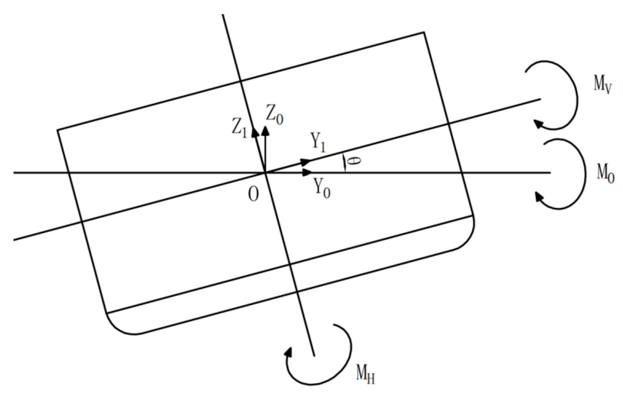
Ships may encounter various types of dangers at sea; for instance, list due to stranding or hull damage due to collision. The Ro-Ro ship Modern Express underwent an accident in 2016, and floated at sea for more than one week with a list angle of 51 degrees. Compared to ships floating in the upright position, the hydrostatic load acting on a damaged ship is very different. When a ship is in a listed position, the horizontal bending moment, in addition to the vertical bending moment, must be also considered in the body-fixed coordinate system. If the ship hull is also damaged, the strength of the hull girder will be impaired, and the ship will be in a more dangerous situation. Researches have shown that the horizontal load acting on a damaged ship may be as large as 1.73 times the vertical load [1,2]. For this reason, the assessment of ship strength is more than just about dealing with the vertical bending moment; in fact, the ultimate limit state function of the ship under the action of combined loads must be assessed.
To investigate the ultimate limit state function, the ultimate strength must be calculated first. The existing methods for calculating the ultimate strength of the hull girder can be categorised into two groups: analytical methods and progressive collapse methods [3]. The analytical methods include the elastic analysis method (such as the initial yielding bending moment method) and fully plastic bending moment method (Caldwell’s method [4]). The practices show that these methods are useful for predicting the ultimate strength and residual strength of the hull girder in the early design stage. Based on investigations of the collapse procedure of a ship undergoing the bending moment of a hull girder, some progressive collapse analysis methods have been proposed, such as nonlinear finite element analysis (including the Idealised Structural Unit Method) [5,6] and Smith’s method [7]. The nonlinear finite element analysis, which can simultaneously consider yielding, buckling and the mixed failure behaviour of structural elements constituting the hull girder, is recognised as the most reliable approach for calculating the ultimate/residual strength. However, its application is limited due to the huge modelling and computing time, and also the requirement of the engineer’s experience [8,9]. Meanwhile, a progressive collapse method was proposed by Smith [7], by which, the cross-section of concern is discretised into units of stiffened panels, then the curvature of the hull girder is increased step by step, and the nonlinear behaviour of each unit is obtained by analysing its stress–strain relationship so as to obtain the section bending moment at different curvatures of the hull girder. This method has been widely used in the community, and is referred to as the Smith Method [10]. Hence, the simplified progressive collapse method is adopted for the ultimate strength analysis in this study.
The accuracy of the Smith Method relies on the stress–strain relationship and the calculation of the neutral axis. There exist quite a few researches on the stress–strain relationship. Hughes et al. [11] investigated the failure behaviour of various types of stiffened panels using an incremental iteration method, and the comparison with experiment showed fair accuracy. Yao [12] derived the stress–strain relationship for the coupled flexural–torsional behaviour of angle bar stiffeners. HCSR [10] also provided various stress–strain relationships for the calculation of the ultimate strength of hull girders. However, the relationships provided by HCSR were derived using the compression and tension equilibrium in the structure above and below the neutral axis that is parallel to the water line, and they cannot be applied to asymmetric cross-sections due to inclination and/or hull damage. In the case of an asymmetric stress–strain, the neutral axis does not only translate, but also rotate. Fujikubo et al. [13] found that the influence of the rotation of the neutral axis on the accuracy of residual strength may be as large as 8%. In order to account for the rotation, Joonmo et al. [
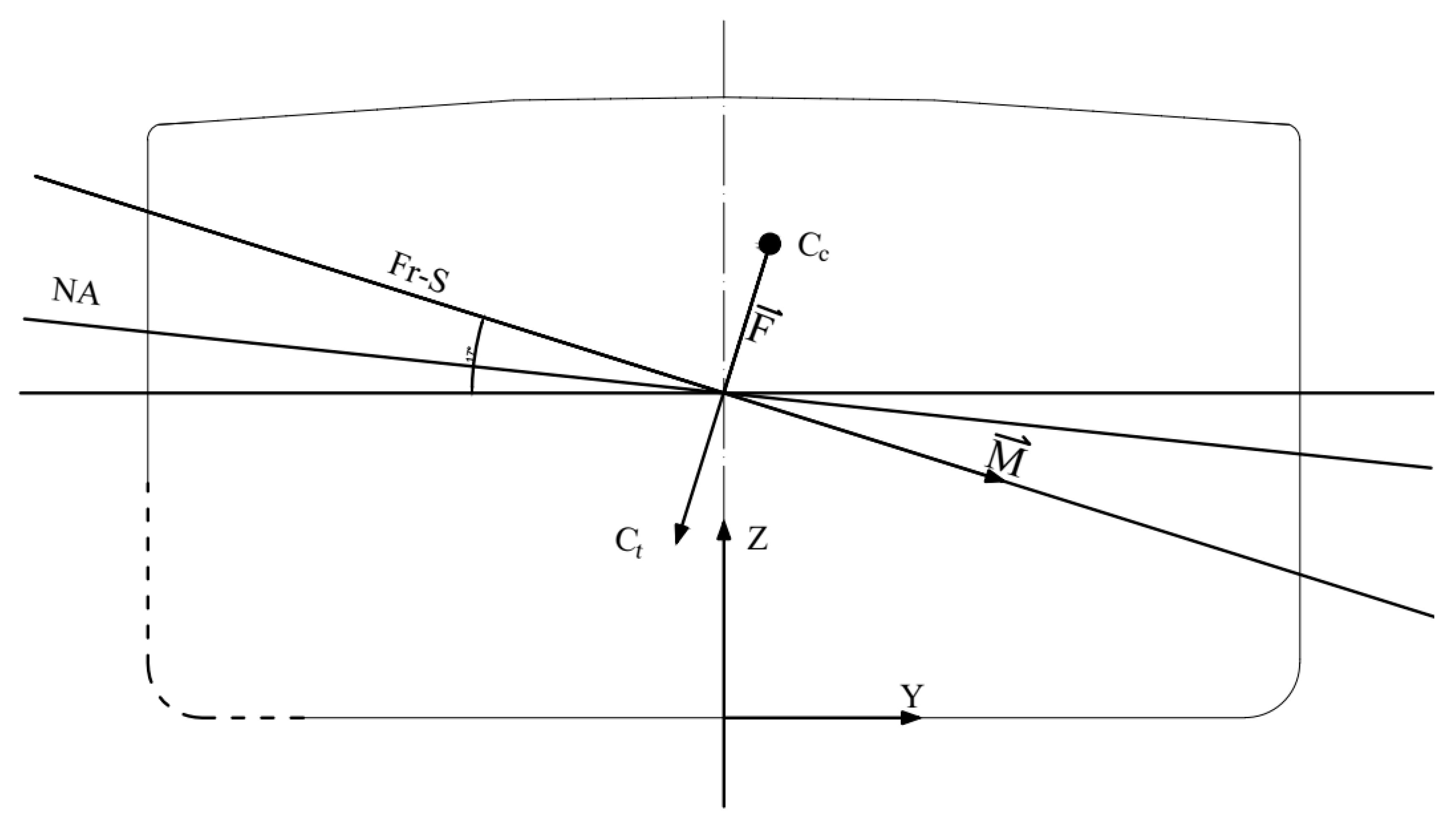
14] proposed a force vector equilibrium method where both the force and moment at the cross-section are in equilibrium.
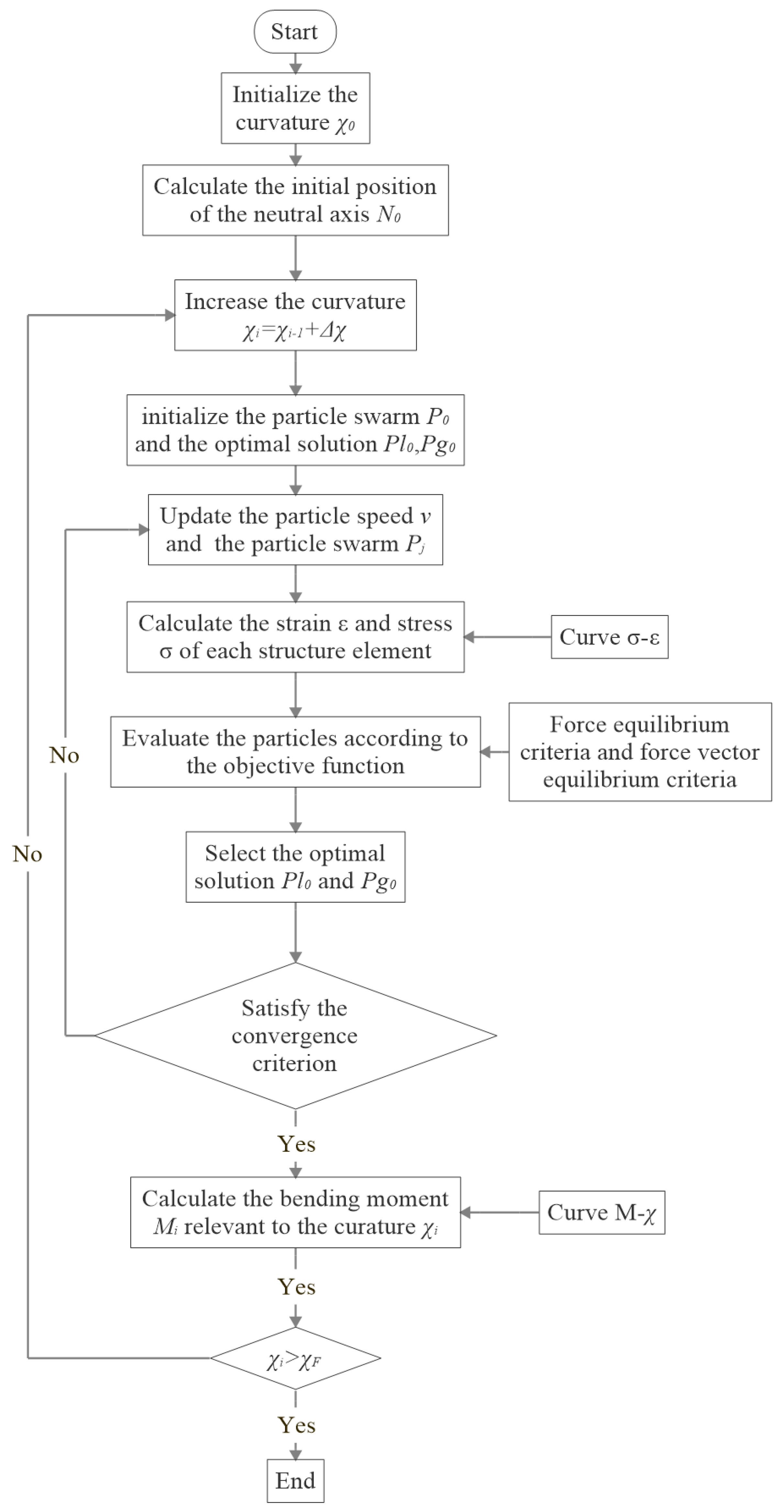
Although theoretically, the instantaneous position of the neutral axis can be accurately determined by the equilibrium both in force and force vector, a proper numerical method is required for the convergence of a solution. Li et al. [15] proposed a linear search method to obtain the solution. However, the translation and rotation are dealt with separately in the iteration process, and certain experience is needed to obtain reasonable results.
The solution to the instantaneous position of the neutral axis is a problem of seeking the optimum solution, and for which there exist a number of algorithms, such as Particle Swarm Optimisation (PSO) [16], ant colony optimisation [17], genetic algorithm [18] and simulated annealing [19]. Among these algorithms, the PSO algorithm was inspired by the social behaviour of bird swarms. Massless and volumeless particles are adopted to represent individuals of the swarm, and each individual is a solution. The motion of each of these particles obeys a simple law, and the global optimum solution is searched in the solution space, accounting for the influences between the particles. This algorithm is widely applied in many engineering areas for its simple implementation, fast convergence, and excellent accuracy. Li et al. [20] applied the PSO algorithm to trace the instantaneous position of the neutral axis, and both the translation and rotation are dealt at the same time. Comparison of results showed that the accuracy is satisfactory.
Among the researches on the fitting of ultimate limit state function under multiple loads, mostly the combined load of vertical and horizontal bending moments [21,22,23], the following fitting equation is often used.
γ 1 ( M V M U V ) α + γ 2 ( M H M U H ) β = 1 ,
where γ 1 , γ 2 , α and β are the fitting parameters of the function; M V and M H the vertical and horizontal bending moment of the ship in the ultimate state, respectively; M U V the ultimate vertical bending moment when the ship is in a sagging or hogging state; and M U H 
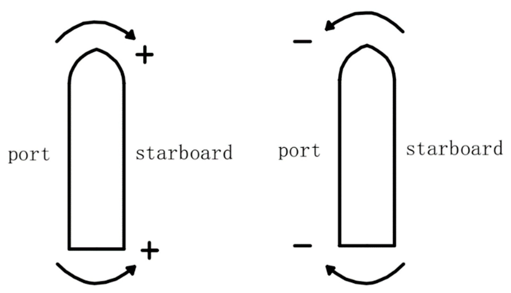
the ultimate horizontal bending moment when included to port or starboard. These parameters vary from one to another, and Table 1 shows some of them used by researchers for intact ships.
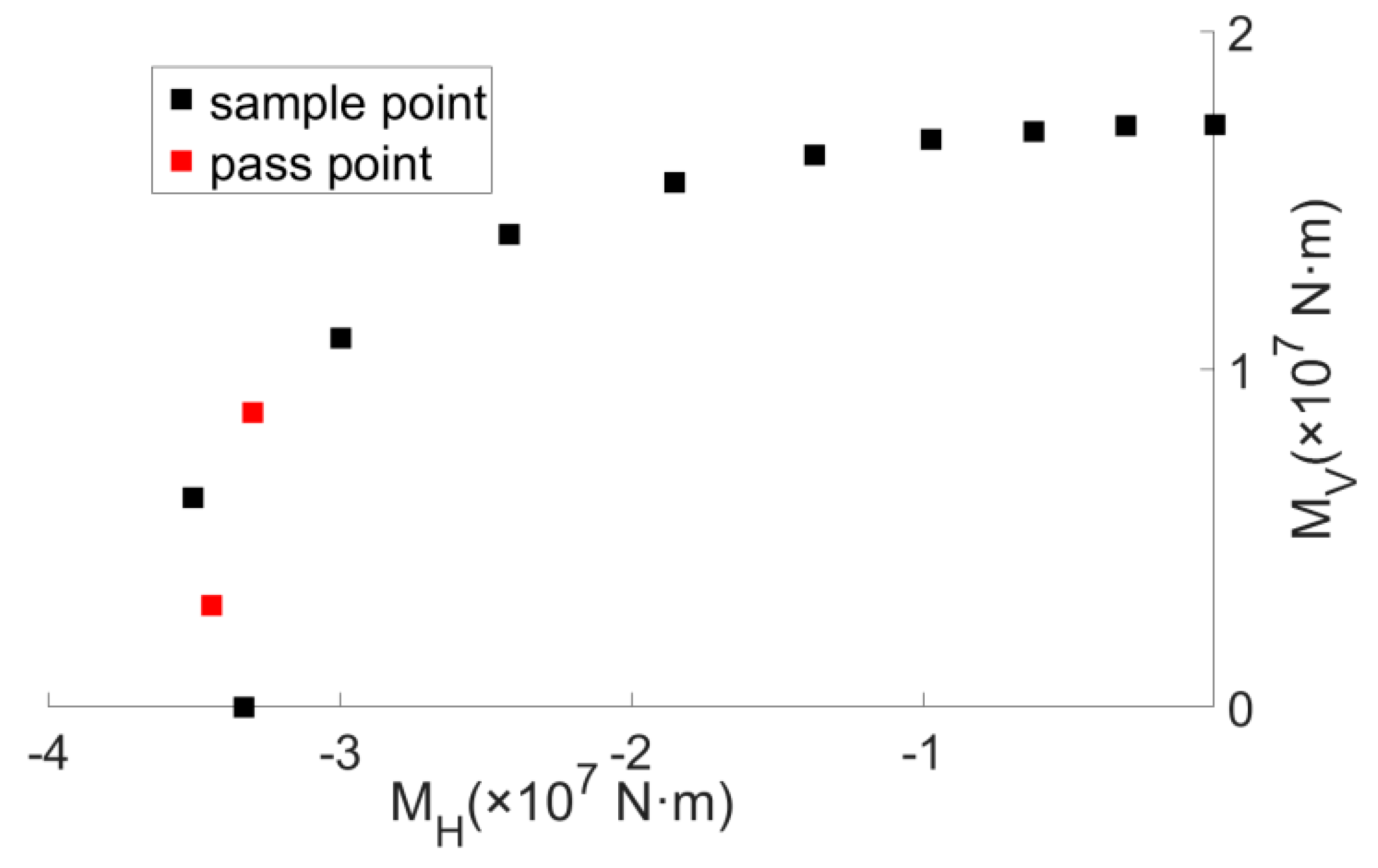
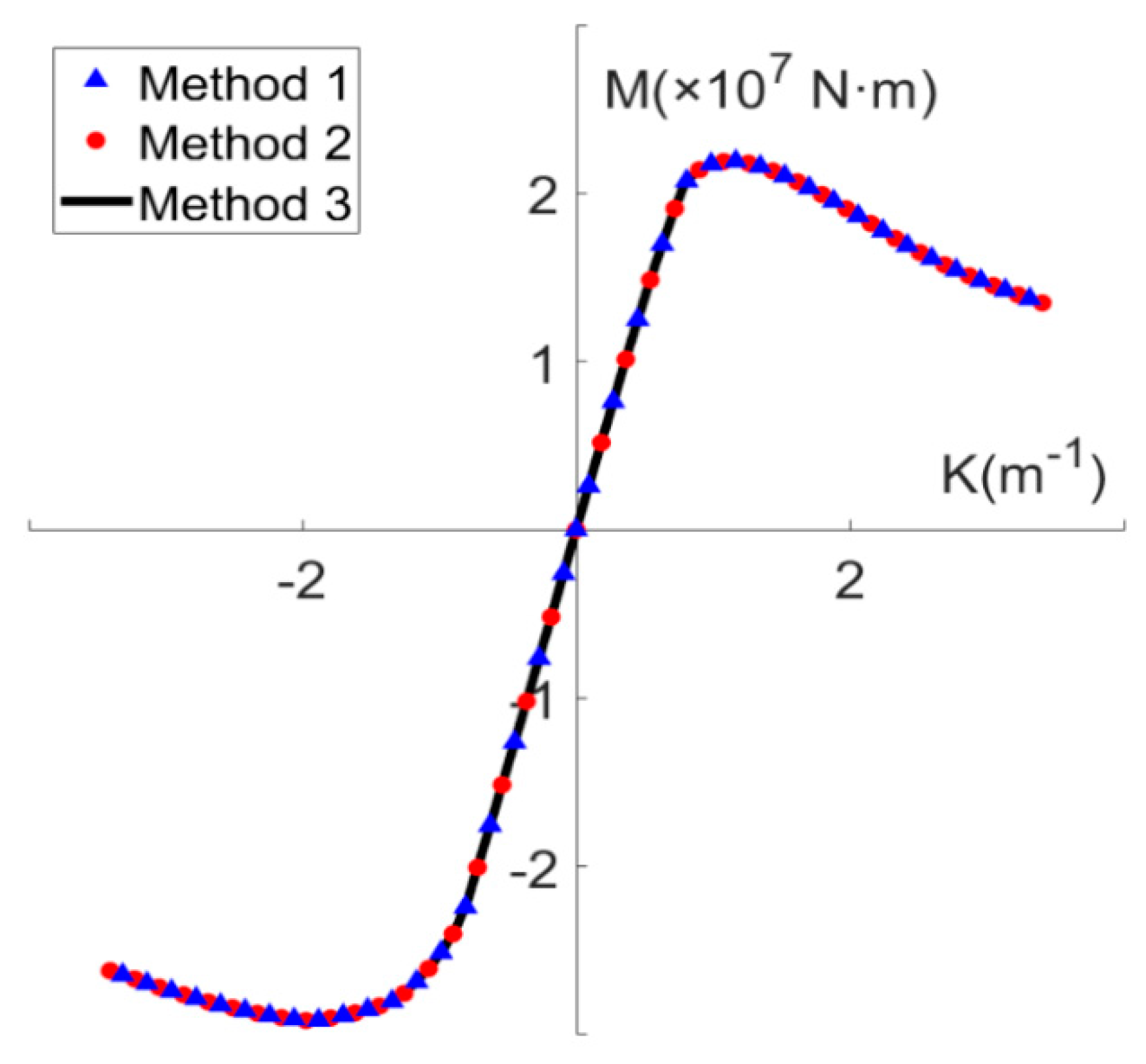
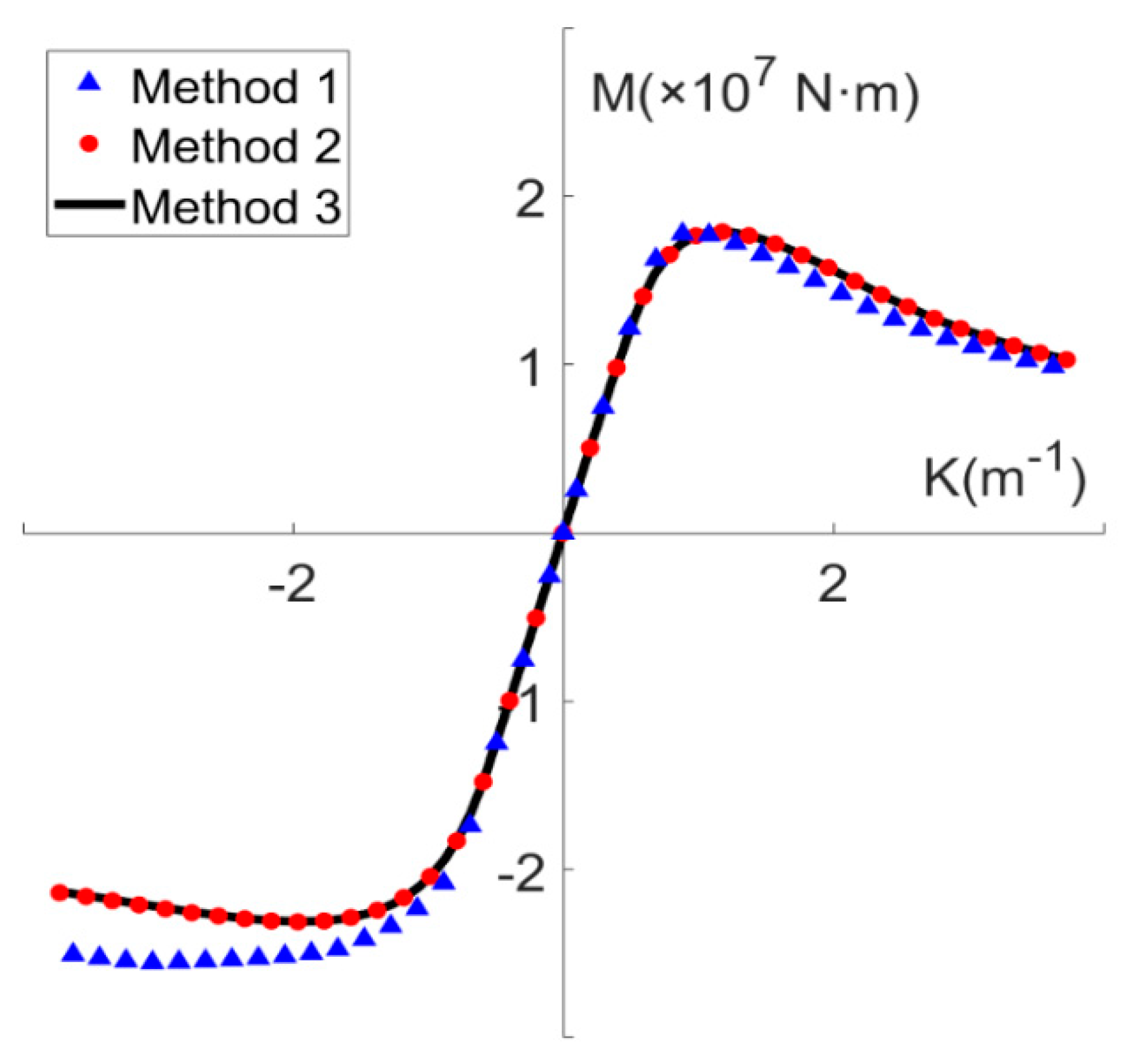
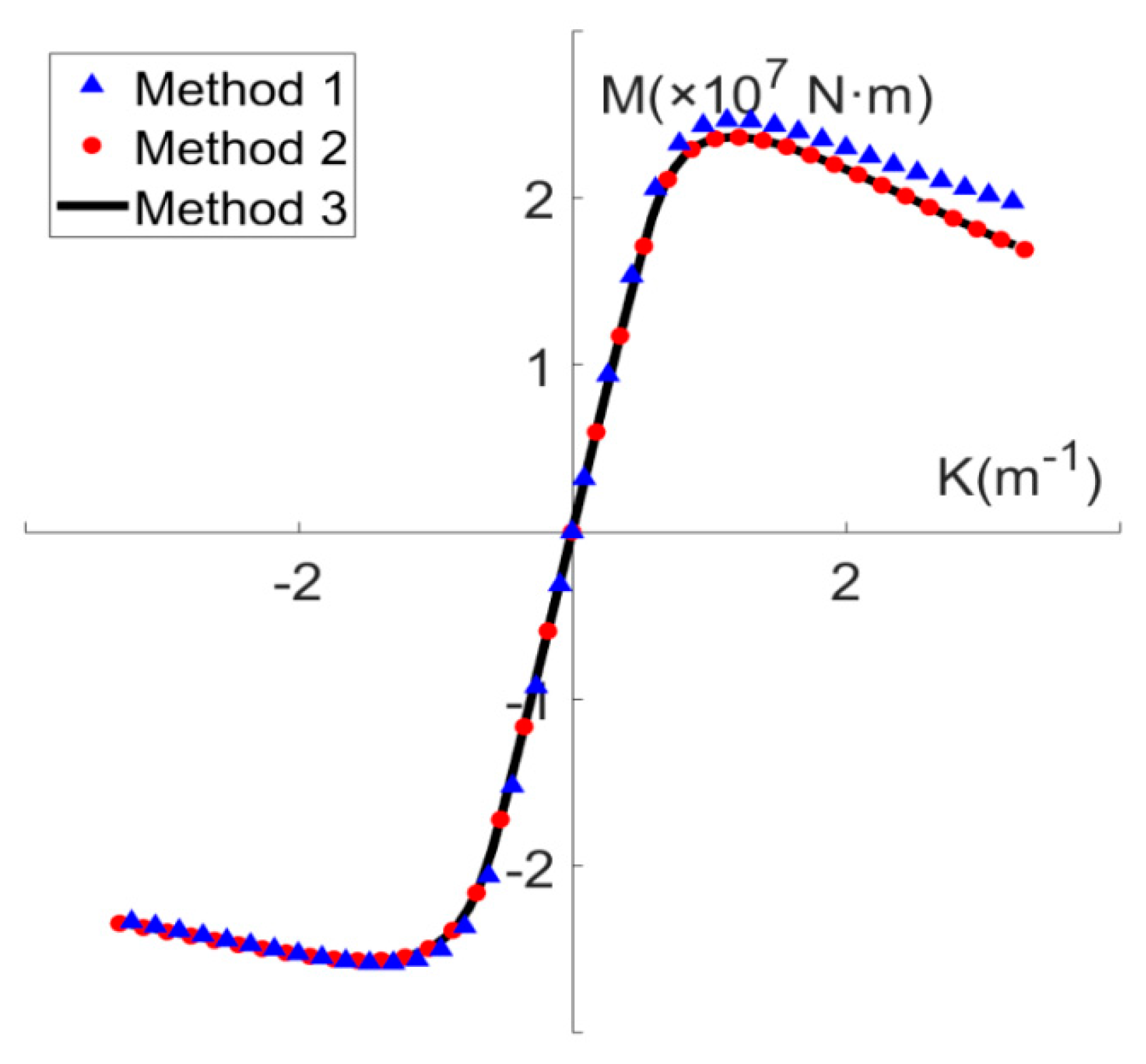
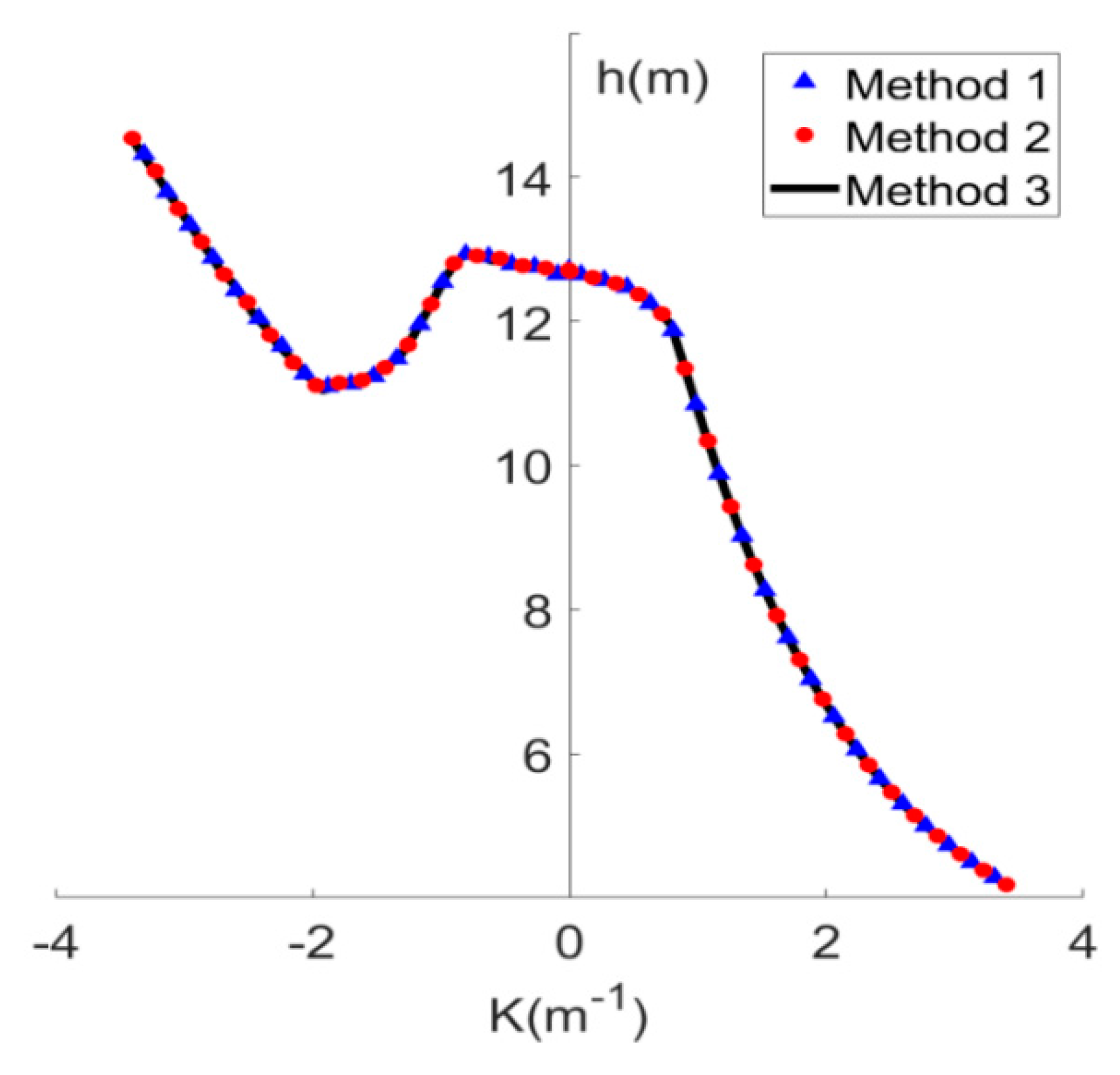
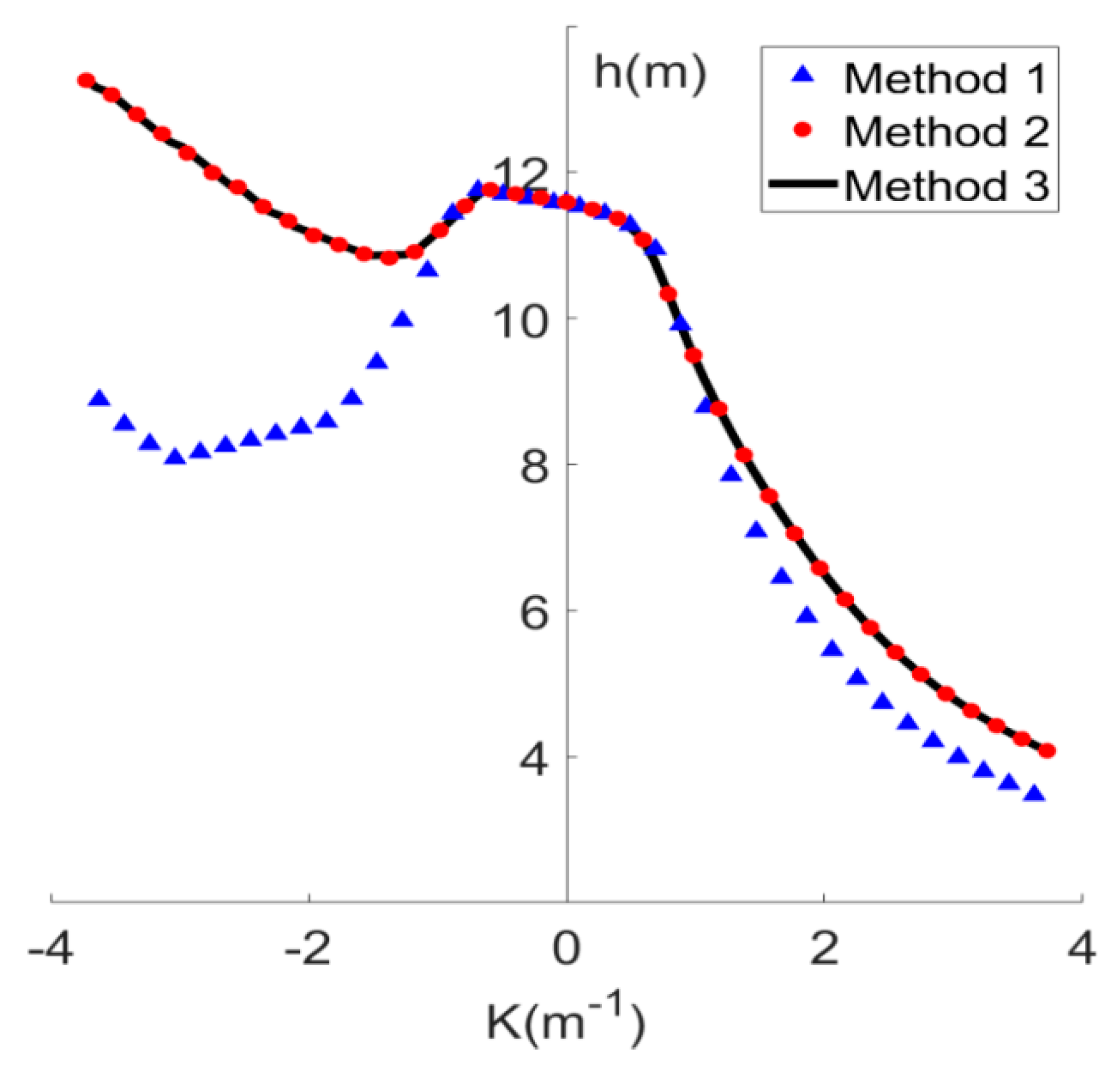
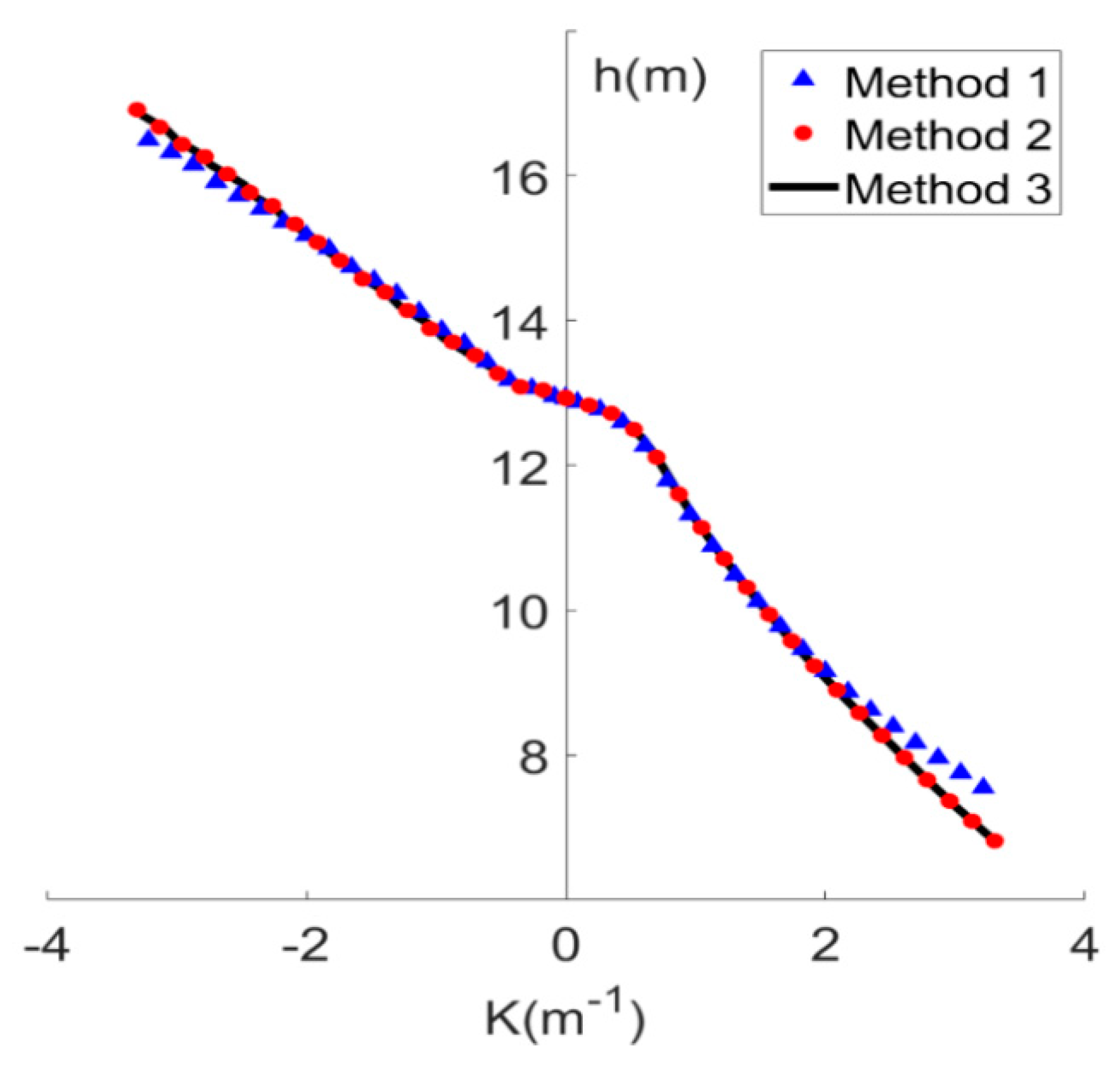
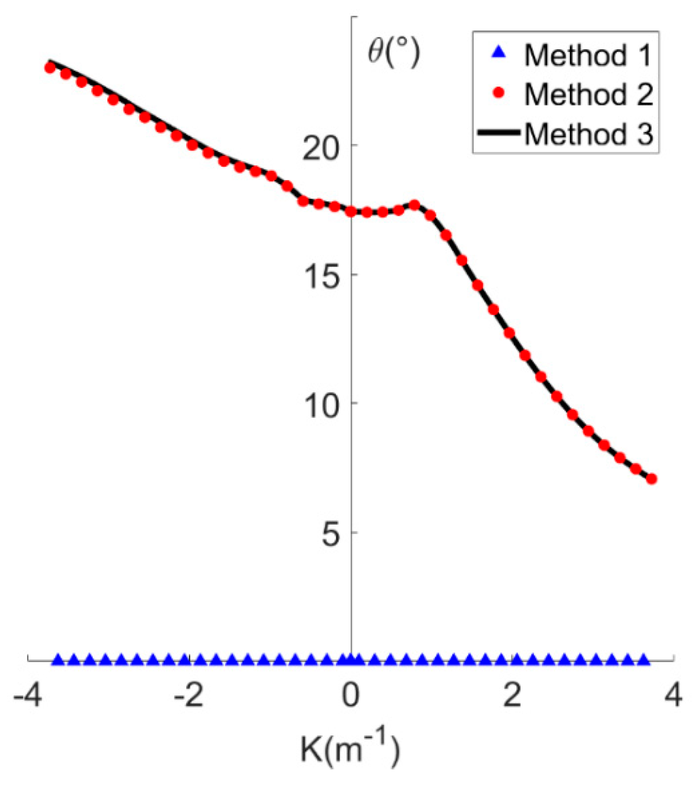
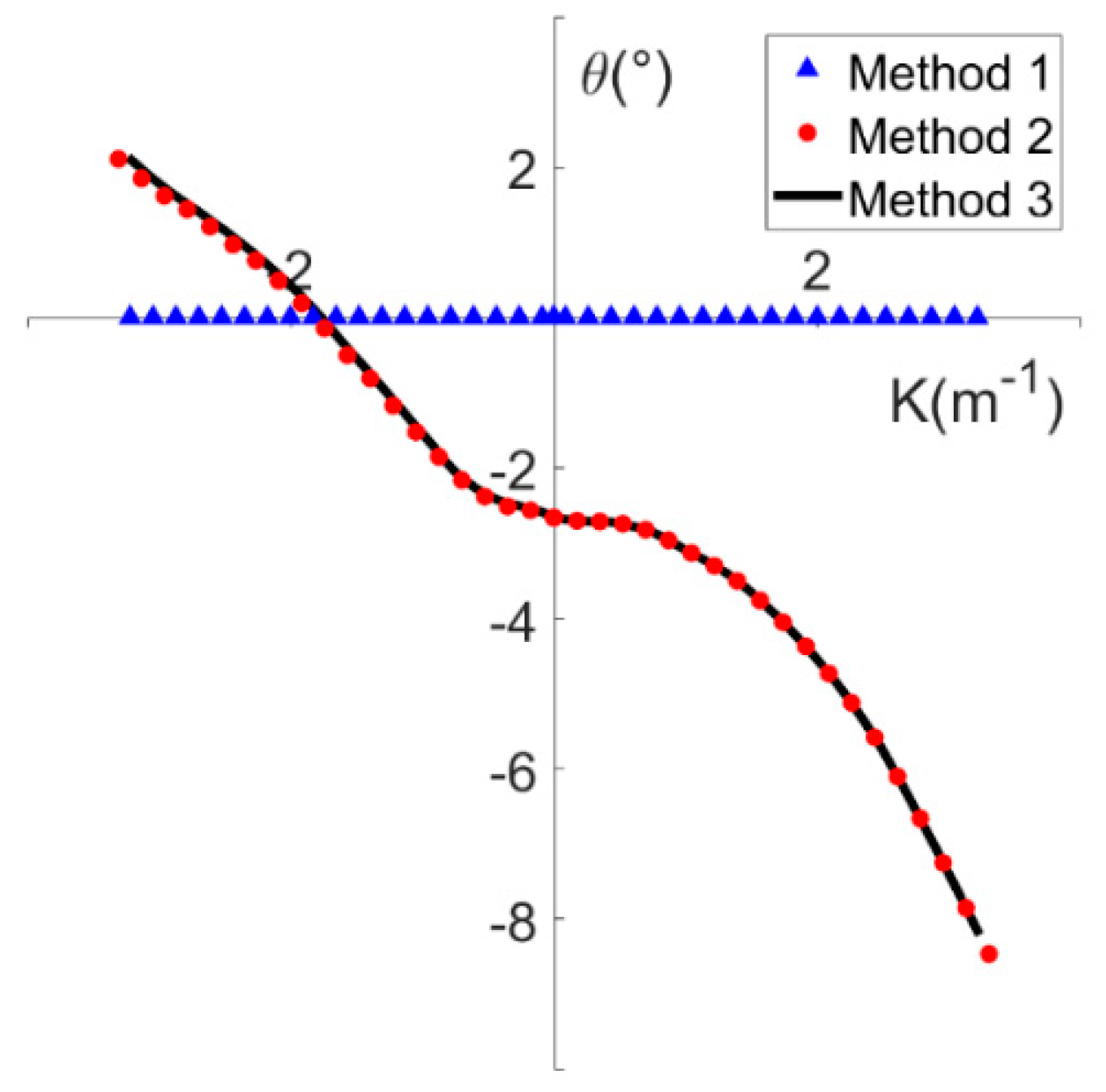
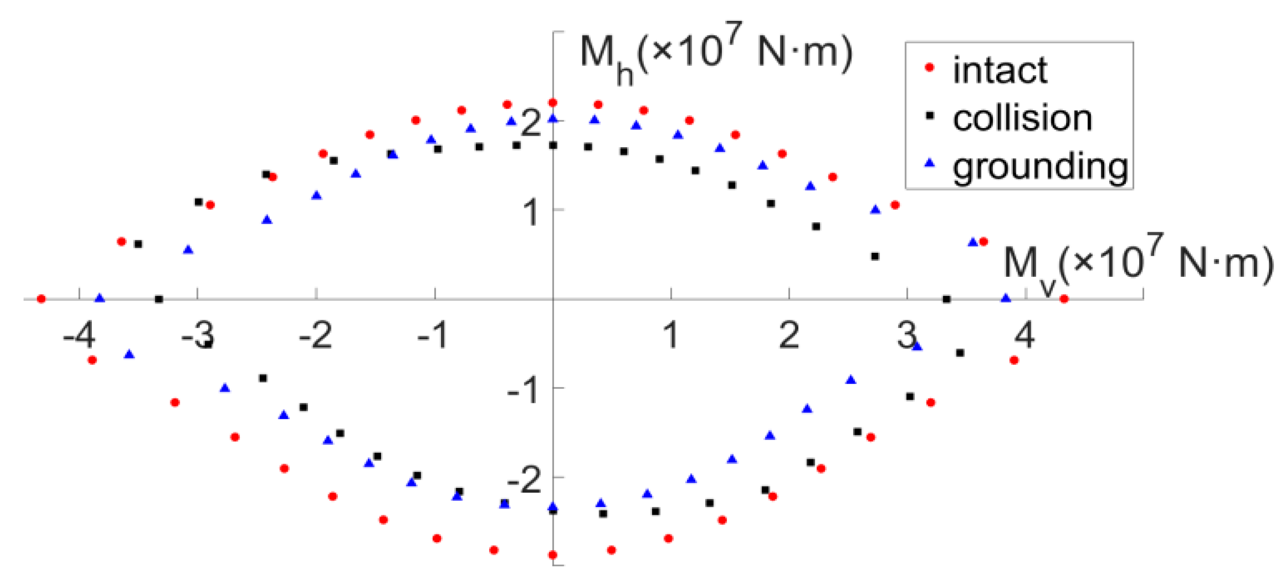
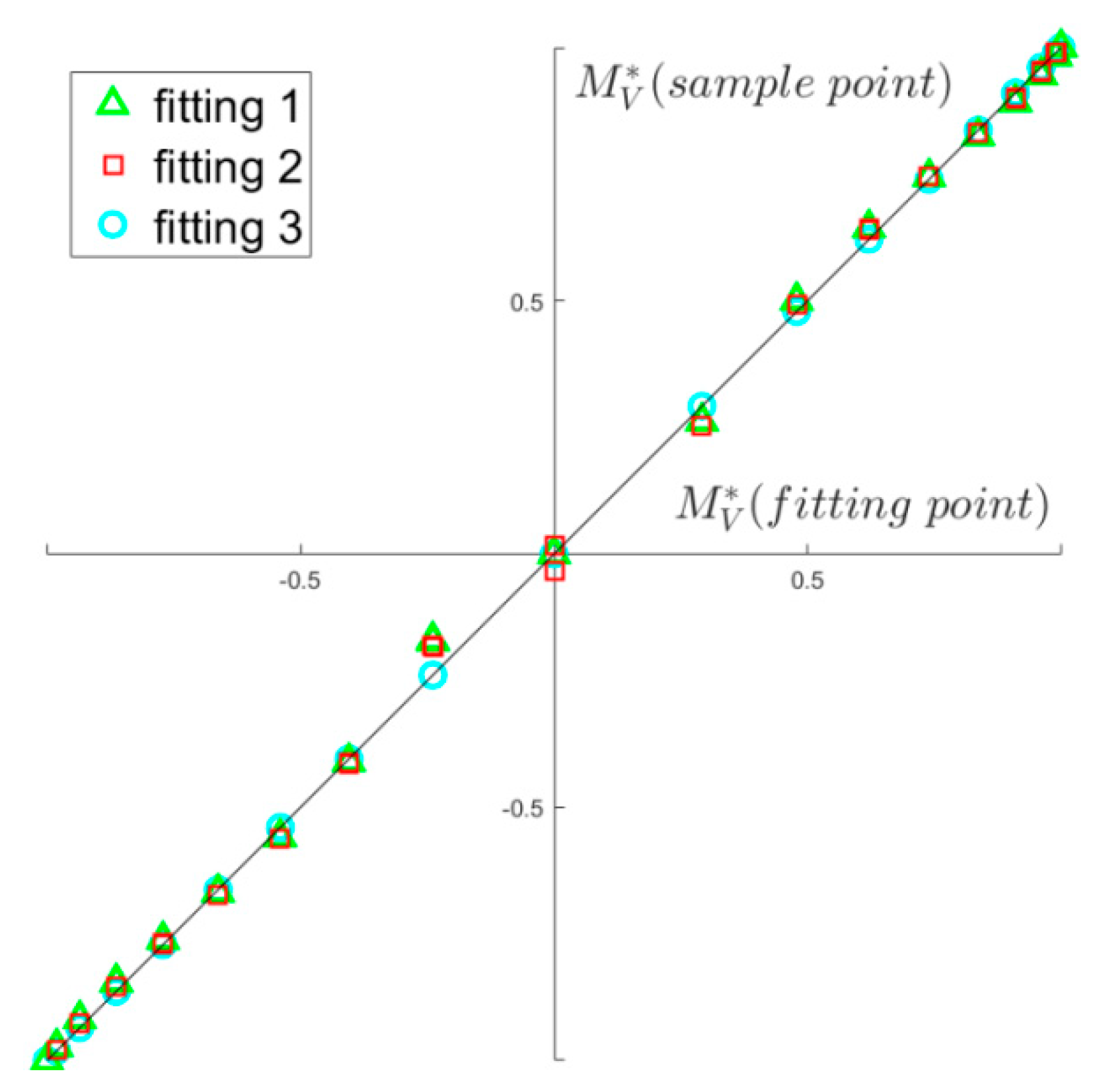
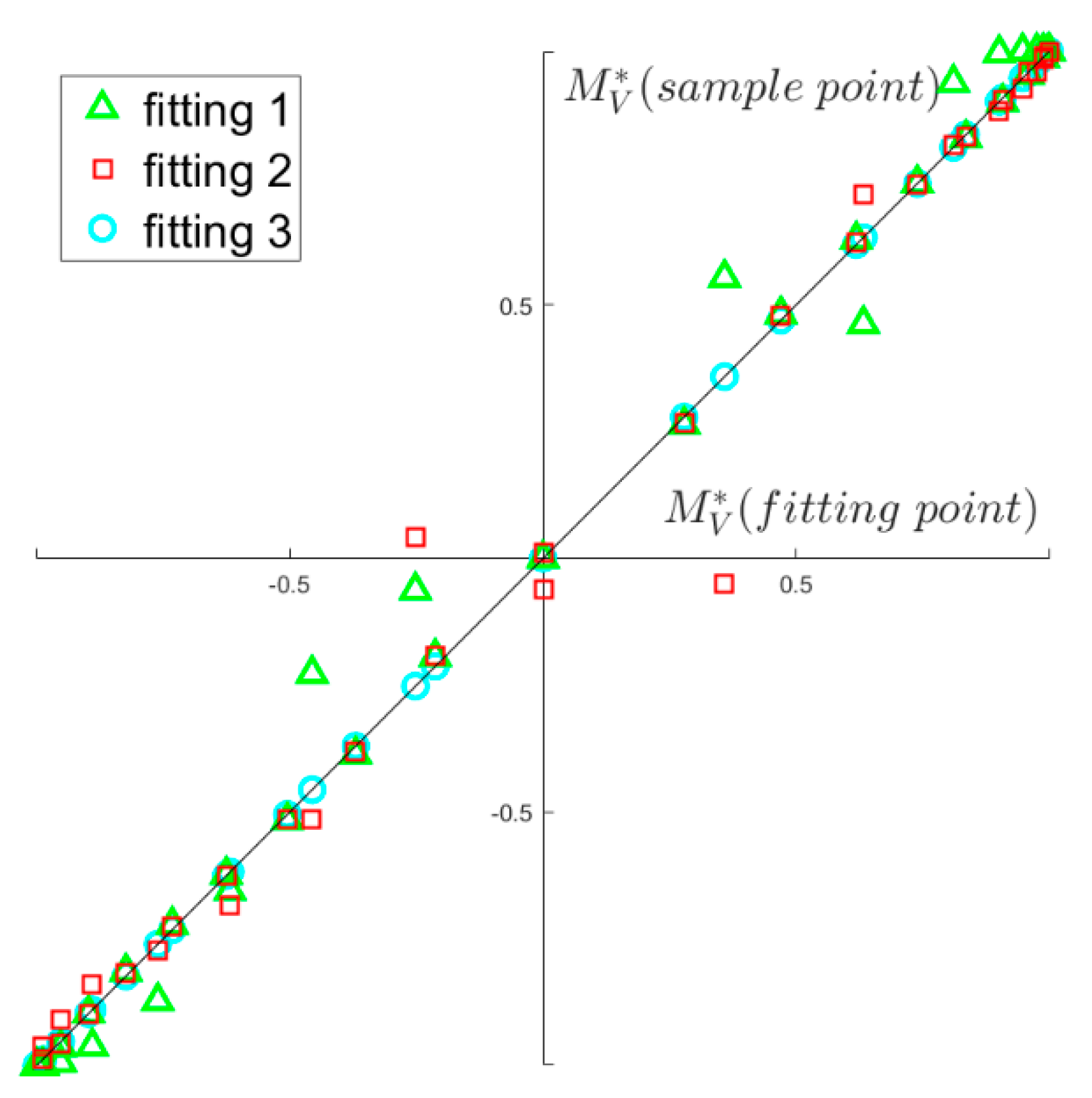
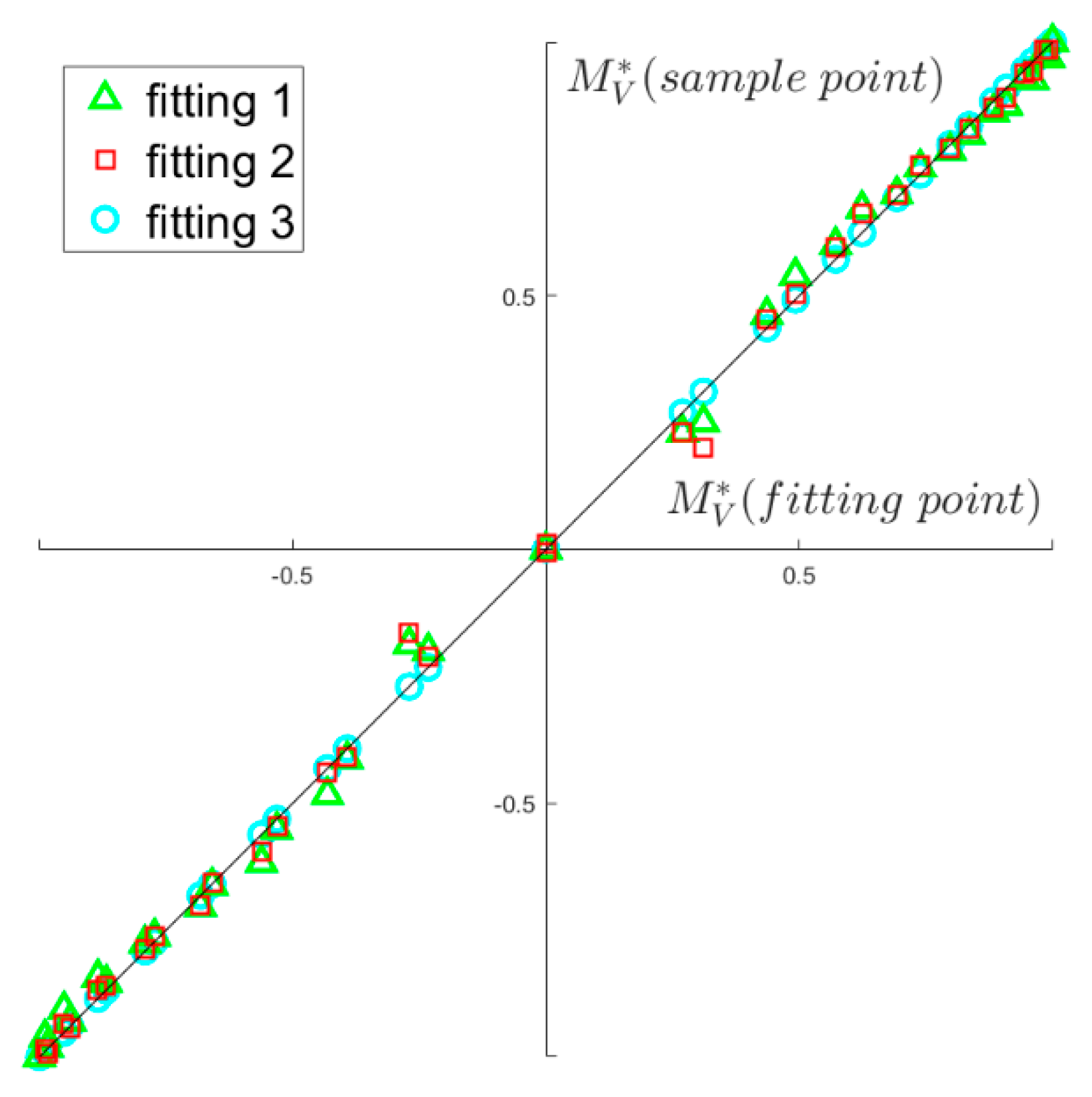
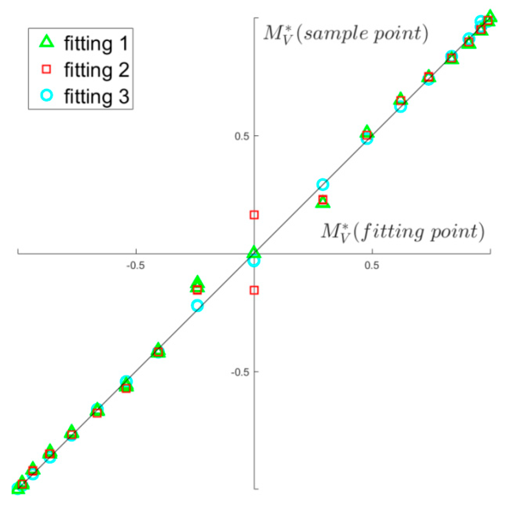
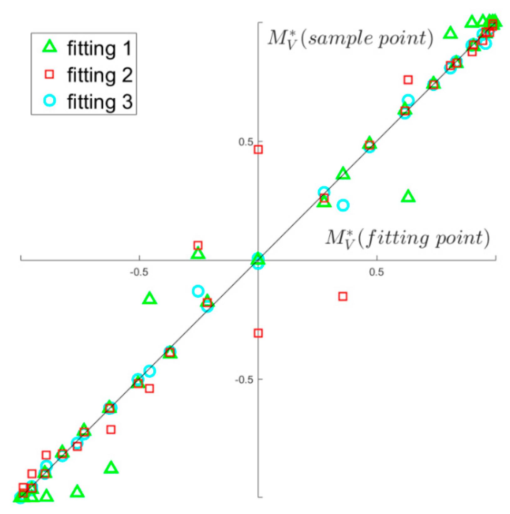
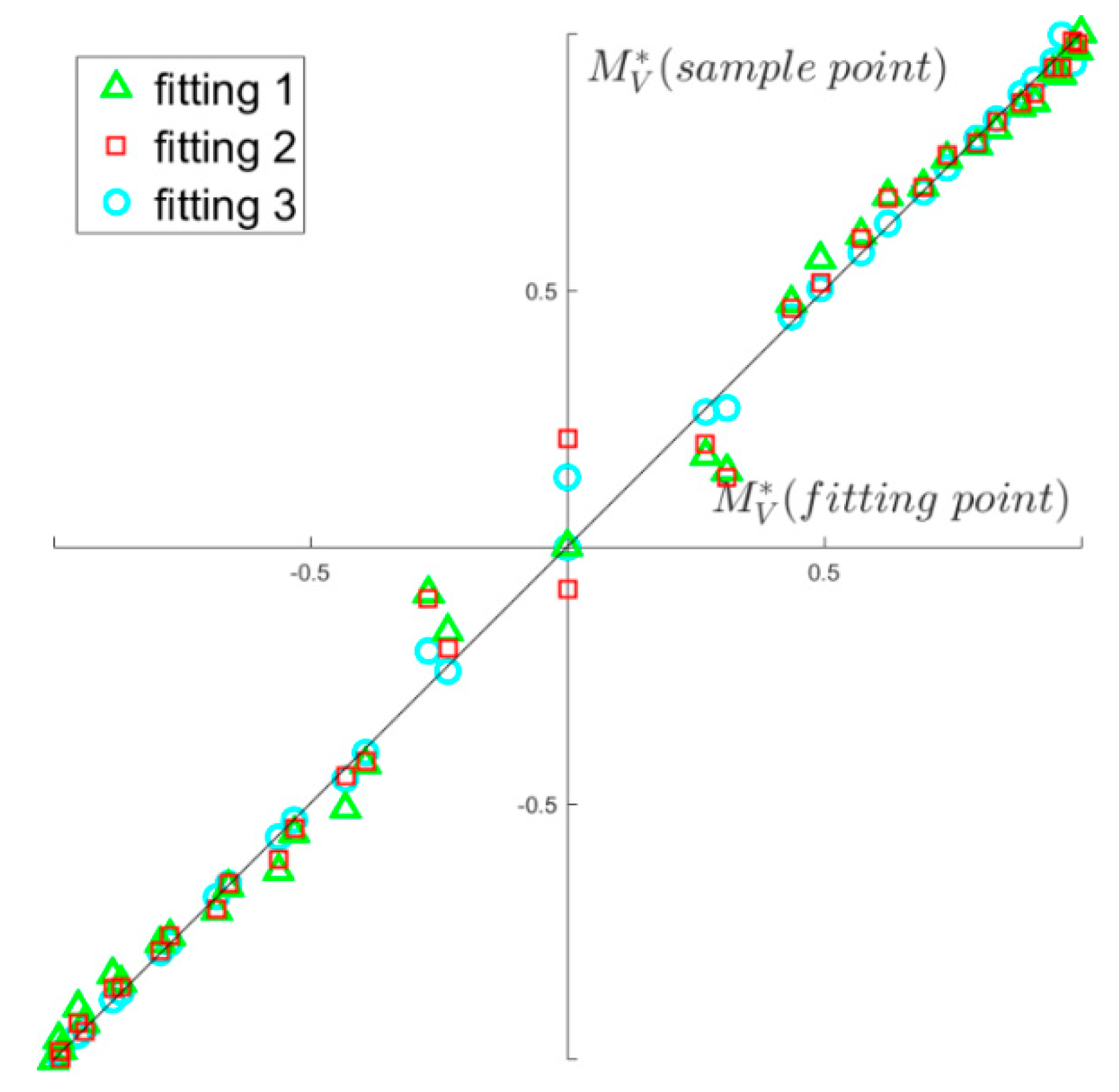
It can be seen in Table 1 that attempts have been made to obtain a function to describe the coupling relationship between the two bending moments. The fitting is satisfactory when the samples of bending moments bear a negative relationship with the absolute values; however, if the samples bear a positive relationship, it will be very difficult to obtain a fitting function with desired accuracy, as shown in Figure 1, where the trend of the samples starts to change when approaching the x axis, and increasing the number of samples is of little help, as shown in Figure 1.
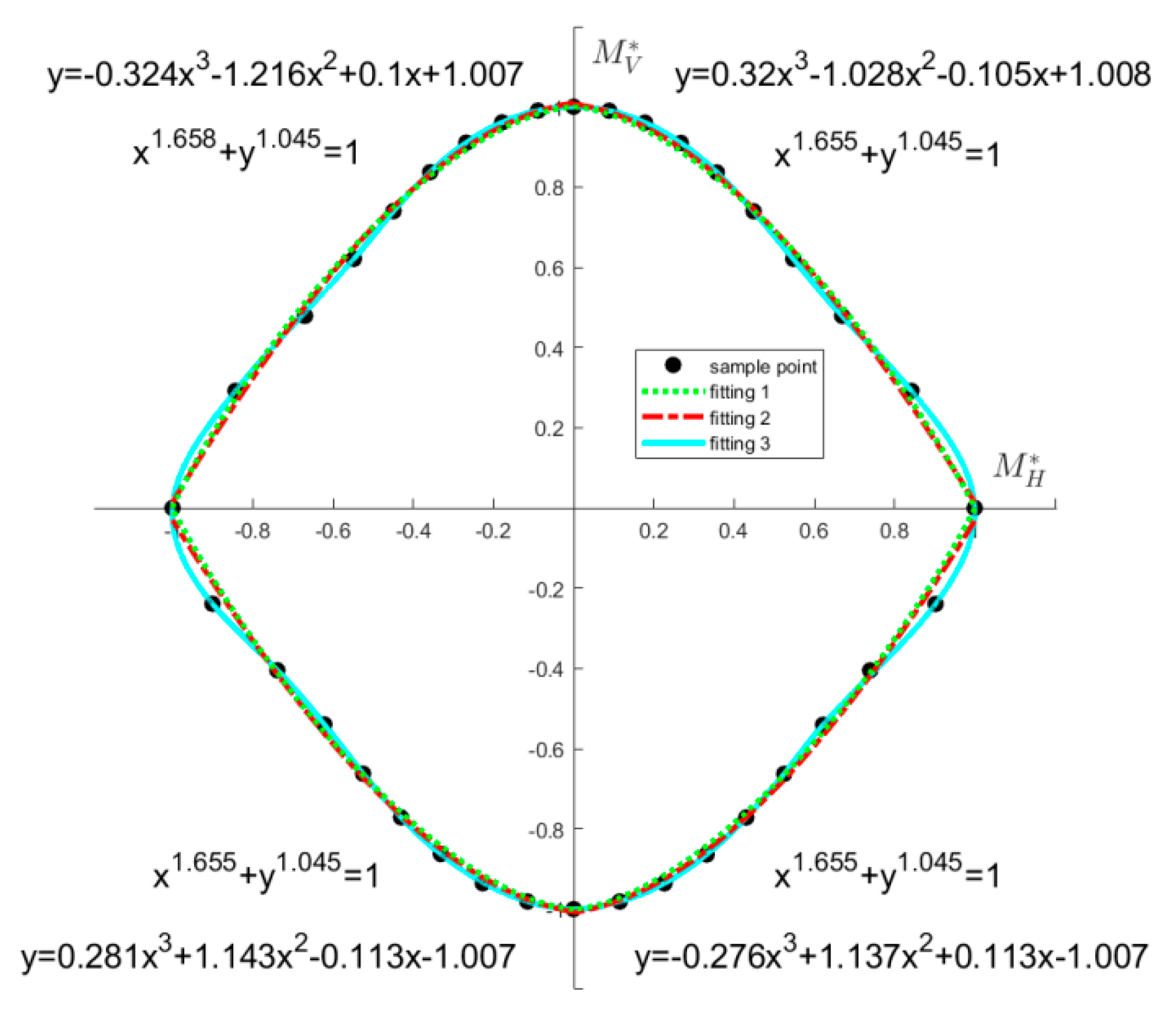
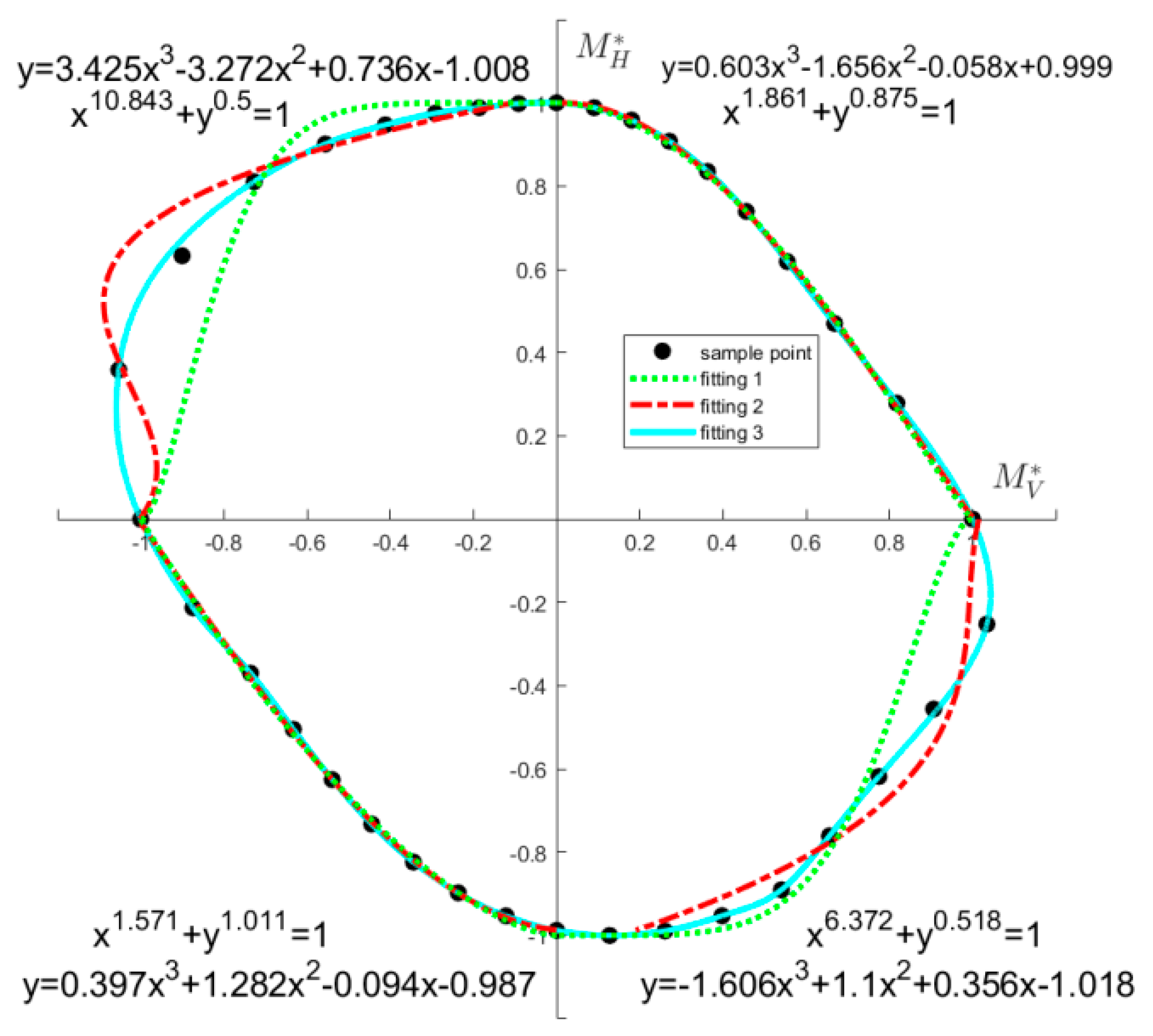
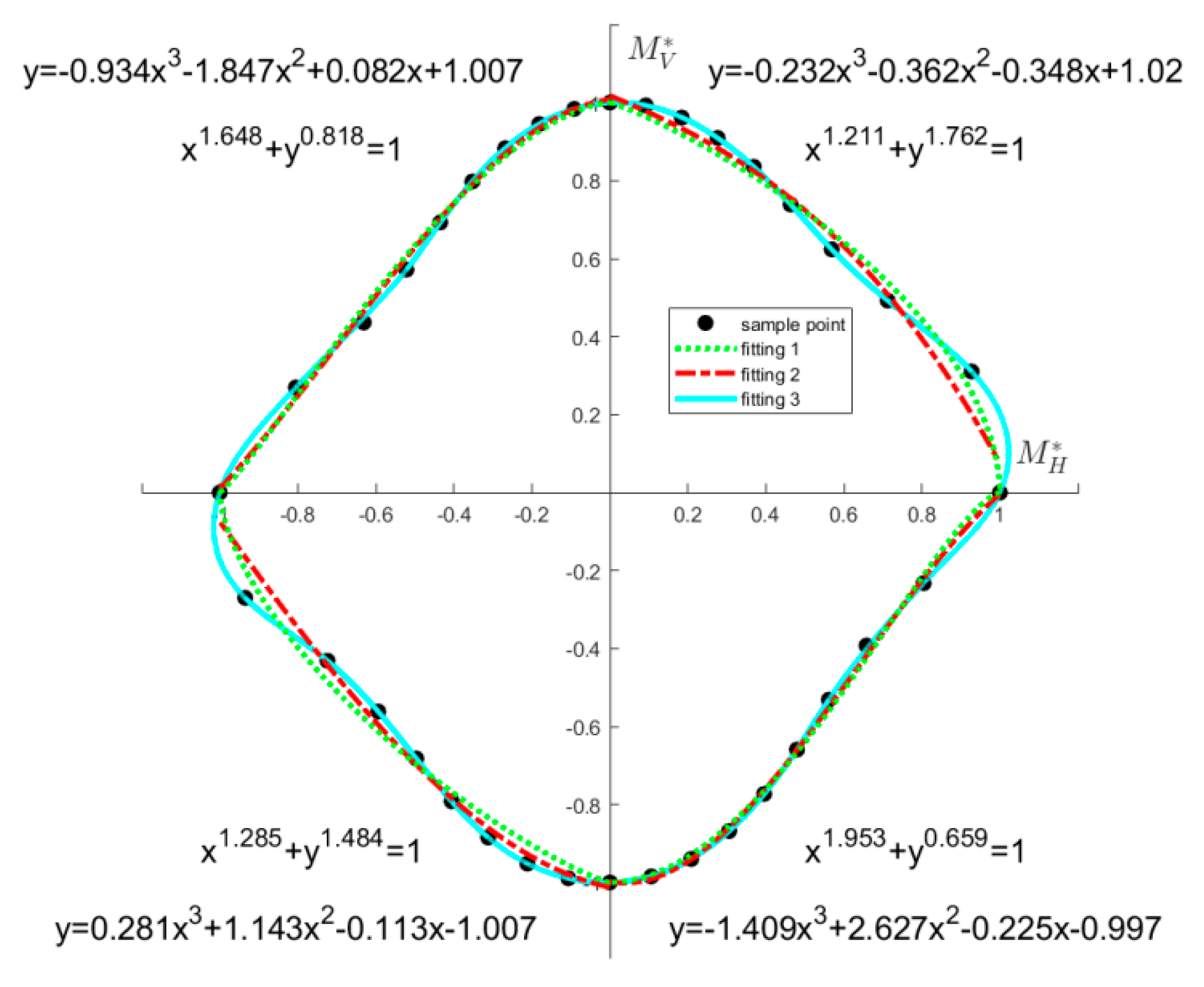
In order to improve the fitting accuracy of ultimate limit state function, Shahid [24] proposed a polynomial fitting method for the case of damaged ships. The polynomial fitting method achieves a quadratic fitting function using multivariable regression. However, it has been shown that there are still some errors in the results obtained with this method. Thus, a new fitting method is desired to accurately describe the relationships between the vertical and the bending moment.
In this study, in order to derive a simple but accurate fitting method, the accuracy of the polynomial fitting method is improved by the means of a piecewise weighted least squared method. With this method, the sample points are divided into groups and fitted separately, then these functions are adjusted by ensuring the continuity at the boundaries, and finally a set of explicit fitting functions are obtained.

2. PSO-Based Smith Method for Ultimate Bearing Capacity Analysis of Damaged Hull Girder

2.1. Smith Method and the Neutral Axis of Asymmetric Section of Damaged Ship

The Smith Method is widely used for the assessment of the ultimate strength of ships, by which, the cross-section of ship hull girder is discretised into units of stiffened panels and hard corner, and the ultimate strength is obtained by an increase of the curvature of the hull girder step by step. The solving process of the Smith Method is introduced in HCSR [10] in detail. The accuracy of the Smith Method relies on the stress–strain relationship and the calculation of the neutral axis.
In most of the cases of an intact ship in an upright floating position, there exist three symmetries: symmetry in geometry, symmetry in material, symmetry in load. Intact ships are usually symmetrical in geometry and material, and the most common two types of asymmetry are:
(1)
Geometrical asymmetry of damaged ships;
(2)
Load asymmetry due to an uneven distribution of goods, the flooding when the hull is damaged, or due to combination of the horizontal and vertical wave bending moments.
To apply the Smith Method, the position of the neutral axis must be determined. The convergence factor provided by HCSR for determining the position of the neutral axis takes the form
| F c F t | | F c + F t | ξ T ,
where F c is the sum of the compressive forces of all units, F t the sum of the tensile forces of all units, and ξ T is the convergence factor for force equilibrium, which is usually smaller than 0.01.
It can be seen that Equation (2) is applicable only when all the three symmetries are present. Absence of any of the three symmetries would result in an asymmetric cross-section. For instance, in the case of a damaged hull, the cross-section is asymmetric due to flooding or loss of goods, and the force acting on it will be as shown in Figure 2. The rotation of the neutral axis is not accounted for in the original HCSR rules, and application of it with any correction will result in a wrong instantaneous position of the neutral axis in this case, which will then introduce errors into the subsequent calculation of the stresses in the units, and eventually lead to an inaccurate solution to the ultimate bending moment.
A new equilibrium criterion is required to determine the position of neutral axis of the asymmetric cross-section. According to the research of Choung et al. [14], an additional force vector equilibrium criterion, in addition to the force equilibrium shown in Equation (2), is to be satisfied:
π 2 ξ R cos 1 ( F M | F | | M | ) π 2 + ξ R ,
where F is the sum of the forces acting on the cross-section, M the total section bending moment, and ξ R the force vector convergence factor (usually smaller than 0.1°).

2.2. The PSO-Based Smith Method

The instantaneous position of neutral axis can be obtained once the equilibrium criteria are met. Since both the transition and rotation need to be accounted for, an appropriate algorithm is required to obtain the solution with fair accuracy. This, actually, is a problem to search for the optimum solution in a given space [20].
In this study, the Particle Swarm Optimisation (PSO) method is used to obtain the solution. The PSO method approaches the optimum solution by collaborating and sharing information between the individuals of a group. Each particle has two properties: speed and location. Speed refers to the speed at which the particle is moving, and location indicates the direction of the motion. The optimum solution obtained for an individual particle is called individual best, while the optimum solution of all the particles is referred to as the global best. According to the individual best and global best, a new calculation is executed to update the speed and location of all the particles. This process is repeated until the convergence criteria are satisfied.
By the Smith Method, the position and rotation of the neutral axis will vary every time the curvature is increased, thus the two motions can be regarded as the two dimensions of the search space. Then the PSO can be applied to seek for the optimum global solution to the objective function. Since the translation and rotation vary at the same time instead of one by one, the actual instantaneous position of the neutral axis at a particular curvature can be obtained in a more direct manner. The flowchart of the PSO-based Smith Method, referred to as the improved Smith Method hereafter, is shown in Figure 3.

3. Fitting for the Ultimate Limit State Functions of Damaged Ships under Combined Bending Moments

3.1. Explicit Ultimate Limit State Functions

The curve of the ultimate limit state function indicates the ultimate vertical and horizontal load carrying capacity under combined load. It is difficult to accurately describe the curve in an explicit form. For this reason, the function is usually obtained by fitting with a number of samples.
Since it is a load combined from bending moments in two directions, i.e., vertical and horizontal, the rotation of the cross-section may be achieved by rotating the coordinate system. In this study, the improved Smith Method is applied to obtain the ultimate bending moment at each rotation. The corresponding ultimate rotation can then be decomposed into components in the axis directions to obtain the vertical and horizontal ultimate bending moment, as shown in Figure 4, where Y 0 O Z 0 is the global coordinate system; Y 1 O Z 1 the body-fixed coordinate system; θ the rotation; M 0 the total bending moment; and M V , M H the vertical and horizontal bending moment respectively, which can be calculated from M 0
{ M V = M 0 cos θ M H = M 0 sin θ ,
The double hull Very Large Crude Container (VLCC) model provided by ISSC [25] is used in this study. In order to guarantee the accuracy, the calculation is performed at every 10 degrees of rotation, and the result obtained for the total ultimate bending moment is decomposed into a vertical bending moment and a horizontal bending moment. The definitions of the horizontal bending moment components are shown in Figure 5. The vertical bending moment y i and the horizontal bending moment x i are obtained for each sample point.
The following equation [23,26] is often used for the explicit fitting.
( M H M U H ) α 1 + ( M V M U V ) α 2 = 1 ,
where M U V and M U H are the ultimate bending moment resulted from pure vertical and horizontal bending in the global coordinate system, respectively. It can be written in the form
x α 1 + y α 2 = 1 ,
where x = M H / M U H and y = M V / M U V .
It can be seen that this is a nonlinear function, and which will be fitted using a nonlinear least square method in this study. This fitting method seeks the best match for the fitting function and determines the unknown coefficients via the least square of errors.

3.2. The Polynomial-Fitting-Based Ultimate Limit State Functions

A polynomial fitting method was proposed by Shahid [24] for the fitting of relationship between bending moments in different directions. Equation (7) shows the general form of the polynomial fitting function:
Y ¯ = C 0 + i = 1 n C i X i + i = 1 n j = 1 n C i j X i X j + ε ,
where Y ¯ is the estimate of the fitting function for the n random variables X i , C 0 an independent regression coefficient, C i the coefficient of the first order term, C i j the coefficient of the cross-quadratic term, and ε the error between the estimate and the real response.
In this study, the third-order polynomial fitting function is adopted.
y = a + b x + c x 2 + d x 3 ,
where x = M H / M U H and y = M V / M U V . Since concave curves, i.e., multiple-value functions, may appear in some cases, the following form is used instead.
x = a + b y + c y 2 + d y 3 ,
Determination of the unknown coefficients is the key to the solution when applying the method, and, for which, the least square method is usually used.

3.3. The Improved Polynomial-Fitting-Based Ultimate Limit State Functions

For highly nonlinear systems, fitting with a single function usually results in poor accuracy, and increasing the order of the fitting function does not always help. Since the local variations of the samples are relatively small, a piecewise regression method is adopted to improve the accuracy of the polynomial fitting function, i.e., piecewise functions are used to describe the response relationship.
The accuracy can be improved by fitting with piecewise functions, but there still might be some large errors in some cases. For this reason, weights are introduced in order to obtain the optimum fit. To be specific, weights are used to improve the local fitting accuracy of each piece. The unknowns in Equation (8) can be calculated as follows.
{ N } j = ( X T w X ) 1 X T w Y ,
where
{ N } = { a , b , c , d } T ,
[ X ] = [ 1 X 1 X 1 2 X 1 3 1 X 2 X 2 2 X 2 3 1 X m X m 2 X m 3 ]   ,
{ Y } = { y 1 , y 2 , , y m } T   ,
where w is the weight.
Then the weights are modified repeatedly until the accuracy requirement is satisfied. Once the fitting is done for all of the pieces, the values of the fitting functions at both ends of the piece, y i 1 and y i 2 , are obtained, and so are the slopes y i 1 and y i 2 . In order to ensure that the two fitting functions of the two adjacent pieces have the same curvature at the joint, the following boundary conditions are applied:
y i 2 = y ( i + 1 ) 1 = y i ,
{ y i 1 = ( y ( i 1 ) 2 + y i 1 ) / 2 y i 2 = ( y i 2 + y ( i + 1 ) 1 ) / 2   ,
Because it is an enclosed curve, the following boundary conditions are also applied
{ y ( n + 1 ) 1 = y 1 y ( n + 1 ) 1 = y 11 .
The fitting function of each piece can be recalculated once the function values and the slopes at the ends of each piece are determined
{ y 1 = a + b x 1 + c x 1 2 + d x 1 3 y 1 = b + 2 c x 1 + 3 d x 1 2 y 2 = a + b x 2 + c x 2 2 + d x 2 3 y 2 = b + 2 c x 2 + 3 d x 2 2 ,

4. Numerical Simulations and Results Analysis

4.1. The Details of VLCC

The cross-section of a double hull VLCC provided by ISSC [25] is adopted for the investigation; see Figure 6. The types and dimensions of the stiffeners are listed in Table 2, and the Young’s modulus and the Poisson ratio are 206 GPa and 0.3, respectively. Typical cases of hull damage due to collision and stranding for the simulation are determined according to the HCSR, and the definitions of the damage are shown in Table 3 and Figure 7.

4.2. Validation of PSO-Based Smith Method

In order to validate the PSO-based Smith Method (Method 3), the ultimate strengths of the three cases shown in Table 4 are calculated, and the results are compared to those obtained with the original Smith Method (Method 1) and the linear search-based Smith Method (Method 2).
The ultimate strengths of the double hull VLCC in sagging and hogging conditions of each case are calculated with the three Smith methods. The results for the ultimate strengths are shown in Figure 8, Figure 9 and Figure 10, and those for the positions of the neutral axis are shown in Figure 11, Figure 12, Figure 13, Figure 14, Figure 15 and Figure 16. The ultimate sectional bending moments in the sagging and hogging condition of CASE 1 are compared with literature in Table 5, and the results for CASE 2 and CASE 3 are shown in Table 6 and Table 7.
It can be seen that, for CASE 1, the results obtained by the three methods for the bending moment and position of the neutral axis are very close. However, there are some differences between the results for CASE 2 and CASE 3. Particularly, the results obtained with Method 1 bear some differences with those obtained with the other two methods, and among them Method 3 is most accurate. For this reason, Method 3 is used to investigate the ultimate limit state function in this study.

4.3. Calculation of the Ultimate Limit State Function

4.3.1. Calculation of Sample Points

Since it is not possible to accurately predict the conditions of a ship at sea, a fit to the ultimate limit state curve is to be made for the ship under different loading conditions. For which purpose, a number of samples of ultimate vertical bending moments and horizontal bending moments need to be obtained. In this study, the ultimate/residual strengths of the ship under different combined loads are obtained for various heeling angles, and then decomposed into the vertical and horizontal bending moments.
The double hull VLCC mentioned before is used for the investigation. The hull is inclined from 0 to 170° with an interval of 10 degrees in order to guarantee the accuracy without incurring too much computation load. The ultimate/residual hogging and sagging strengths of the intact hull and also the damaged hull due to collision or stranding are calculated for each angle, and the sample points of the ultimate vertical and horizontal bending moment under combined load are obtained. For each case of intact/damaged hull, 36 sample points are obtained, as shown in Figure 17.
It can be seen in Figure 17 that, in the case of an intact hull, the ultimate bending moment envelope curve is smooth and approximately symmetric; however, in the cases of a damaged hull, there are abrupt changes in the distribution of the samples, and the curves are not symmetric, particularly in the second quadrant where the horizontal bending moment acting on the inclined ship is even larger than the horizontal bending moment under pure horizontal load.

4.3.2. Fitting Results

The fitted curves which obtained the three methods are shown in Figure 18, Figure 19 and Figure 20, where the results are nondimensionalised by dividing them by the pure bending moment. In these figures, Sample point represents the nondimensional results, Fitting 1 the explicit method, Fitting 2 the polynomial fitting method, and Fitting 3 the improved polynomial fitting method. Since the values of the sample points must be positive in the explicit methods, the absolute values are used here. Because the samples points are distributed in all the four quadrants, and they cannot be fitted with these fitting methods using one function, the fitting is made to the sample points located in the same quadrant with the two on the adjacent axes (10 sample points in total). Thus, four fitting functions are obtained for each case.
The results obtained with the three methods for the fitting for the sample points are shown in Figure 21, Figure 22 and Figure 23. In order to compare the accuracy of the fitting in the ranges outside the sample points, the sample points are removed and the results are shown in Figure 24, Figure 25 and Figure 26.
In order to compare the accuracy of the fitting methods at the sample points, the actual vertical bending moments and the fits to them are plotted in Figure 21, Figure 22 and Figure 23, where the abscissa is the fit to the vertical bending moment, and the coordinate is the actual bending moment. If the point is located on the y = x line, it means that the fit is equal to the actual bending moment; and if the larger is the distance between the point and y = x , the larger is the difference between the fit and the actual bending moment.
To compare the accuracy of the fitting in the ranges outside the sample points, the fitting is made with the sample point of concern removed; i.e., the sample point is removed, and the fitting is made with the remaining sample points. The vertical bending moment is obtained by substituting the horizontal bending moment of this sample point into the corresponding fitting function, and then compared with the actual vertical bending moment. The same is done for all the sample points, and the comparisons are shown in Figure 24, Figure 25 and Figure 26, where the abscissa is the vertical bending moment calculated from the fitting function, and the coordinate is the actual moment.
In order to evaluate the goodness of fit obtained by each method, the coefficient of determination R 2 is calculated using
R 2 = 1 ( y y ^ ) 2 ( y y ¯ ) 2
where y is the fit, y ^ the actual value, and y ¯ the mean of y ^ . The maximum of R 2 is 1, and the closer R 2 is to 1, the better is the fit. The results obtained for the three cases are shown in Table 8, Table 9 and Table 10. In this study, a fitting method is considered as satisfactory if R 2 0.999 . The results obtained for the case are given in Table 8, Table 9 and Table 10.

4.4. Discussions

It can be seen that the bending moment is symmetric for the intact ship, but asymmetric for damaged cases. The bending moment of the damage hull is smaller than that of the intact ship; however, some sample points of the damaged case are located outside the bending moment envelope of the intact ship. Fitting for the nondimensionalised bending moment shows that the three fitting methods produce similar results, except that some differences appear when the load is (almost) a pure bending moment. The fitting results are basically those symmetrical about the axes, which means that a symmetry exists for the bending moment in the horizontal plane as well as in the vertical plane (i.e., hogging and sagging bending moments are symmetric). In the cases of the damaged hull, there are some differences between the three methods, particularly, in the results obtained by the classic method and the polynomial fitting method for the second quadrant.
For the case of an intact hull, the bending moment sample points are symmetrical as the cross-section is symmetrical about the centre plane. It can be seen that the bending moments are larger than that of the damaged hull. The sample points of the damaged hull are asymmetric due to the asymmetric cross-section. Especially in the case of a damaged hull due to collision, where the damage is close to the side wall, a clear asymmetric pattern is displayed. Because of the redistribution of stress in the damaged cross-section, some of the bending moments are relatively large and located outside the fitted curve, as shown in Figure 19. Nondimensionalisation of the ultimate bending moments shows that the fitted curve of the samples points of the intact hull is symmetric about the abscissa and also the ordinate. The distribution of the sample points of the stranding case is somewhat asymmetric, but still similar to the case of the intact ship, and this is because the damage is close to the middle of the bottom, and its influence on the vertical bending is limited. However, for the horizontal bending moment, the influence is much more distinct. For the case of collision, the damage is located at the sidewall and part of the deck is missing, and absence of these strong structure members will result in large reduction of the load carrying capacity, and in turn the pattern of distribution is different.
For sample points with small variations, e.g., in the case of the intact hull, all the fitting methods are accurate. However, when there are large variations in the sample points, e.g., in the case of a damaged hull due to collision, the accuracy of Fitting 1 and Fitting 2 is poor, while that of Fitting 3 is still satisfactory. As can be seen in Figure 21, the accuracy of fitting with the explicit method and the polynomial fitting method is poor in the second and fourth quadrant.
Comparison of Figure 21, Figure 22 and Figure 23 with Figure 24, Figure 25 and Figure 26 shows that the fitted points obtained with the corresponding sample points removed are located at larger distances from x = y , and Fitting 3 is always more accurate than Fitting 1 and Fitting 2.
Comparison of the results obtained with and without removing the sample points shows that increase in the number of sample points improves the accuracy, but the improvement is limited in many cases; in particularly, in the case of a damaged hull due to collision.
The results obtained for the goodness of fit also shows that the accuracy of Fitting 1 and Fitting 2 is not always accurate for the case of damaged hull due to collision or stranding, while Fitting 3 is the most accurate in all of the cases.

5. Conclusions

In this study, a PSO-based Smith Method is applied to calculate the ultimate strength of the intact/damaged hull under the combined load of the vertical and horizontal bending moment. A weighted piecewise polynomial fitting method is devised to obtain the ultimate limit state function of ships under the combined load of vertical and horizontal bending moment. Based on the comparison of the results with literature, the following conclusions are drawn.
(1)
Compared to the implementations of the Smith Method, where only the translation of the neutral axis is considered, or the linear search method is applied to trace the position of the neutral axis, the PSO-based Smith Method is more accurate in obtaining the instantaneous position of the neutral axis, and helps produce more accurate results for the ultimate bending moment. Application of the PSO-based method also helps with more accurate fitting of the ultimate limit state functions.
(2)
The weighted piecewise fitting method proposed in this study is more accurate for the fitting of the ultimate limit state function than the explicit method and the original polynomial fitting method, especially in the case of a damaged hull due to collision.
(3)
Comparison of the fitting with and without the sample points removed shows that increasing the number of sample points may help with the accuracy of the explicit fitting and the original polynomial fitting method, but the improvement is limited, and the accuracy is still unsatisfactory in some cases.
(4)
Results obtained for the cases of the intact/damaged hull show that the explicit fitting method and the original polynomial fitting method produce fairly accurate results for the case of an intact hull. Thus, they can be used as the first choices for obtaining the ultimate limit state function of intact hulls for their simplicity, while the weighted piecewise fitting method can be used for the cases of damaged hulls.

Author Contributions

Conceptualisation, C.L.; Methodology, C.L. and X.Z.; Modelling and Computation, Z.Z., Analysis, Z.Z. and C.L.; Writing—Original Draft Preparation, Z.Z.; Editing and Revision, X.Z.; Supervision, C.L. and X.Z.; Funding Acquisition, C.L.; Project Administration, H.R.; Resources, H.R. All authors have read and agreed to the published version of the manuscript.

Funding

The study was supported by the National Natural Science Foundation of China under Grant No. 51779055, 51679055 and 51509058.

Acknowledgments

The authors would like to thank all the reviewers for their valuable comments.

Conflicts of Interest

The authors declare no conflict of interest.

References

  1. Chan, H.S.; Incecik, A.; Atlar, M. Structural Integrity of a Damaged Ro-Ro Vessel. In Proceedings of the Second International Conference on Collision and Grounding of Ships, Technical University of Denmark, Lyngby, Denmark, 1–3 July 2001; pp. 253–258. [Google Scholar]
  2. Chan, H.S.; Atlar, M.; Incecik, A. Global Wave Loads on Intact and Damaged Ro-Ro Ships in Regular Oblique Waves. J. Mar. Struct. 2003, 16, 323–344. [Google Scholar] [CrossRef]
  3. Yao, T.; Fujikubo, M. Buckling and Ultimate Strength of Ship and Ship-Like Floating Structures; Butterworth-Heinemann: Oxford, UK, 2016. [Google Scholar]
  4. Caldwell, J.B. Ultimate Longitudinal Strength. Trans. RINA 1965, 107, 411–430. [Google Scholar]
  5. Valsgaard, S.; Jorgensen, L. Ultimate Hull Girder Strength Margins in Present Class Requirements. In Proceedings of the SNAME Symposium on Marine Structural Inspection, Maintenance and Monitoring, Arlington, VA, USA, 18–19 March 1991; pp. 1–19. [Google Scholar]
  6. Ueda, Y.; Rashed, S.M.H. The Idealized Structural Unit Method and Its Application to Deep Girder Structures. Comput. Struct. 1984, 18, 227–293. [Google Scholar]
  7. Smith, C.S. Influence of Local Compression Failure Compression Failure on Ultimate Longitudinal Strength of Ship Hull. In Proceedings of the International Symposium on Practical Design in Shipbuilding, Tokyo, Japan, 18–20 October 1977; pp. 73–79. [Google Scholar]
  8. Paik, J.K.; Thayamballi, A.K. Ultimate Limit State Design of Steel-Plated Structures; John Wiley & Sons, Ltd.: Hoboken, NJ, USA, 2003. [Google Scholar]
  9. Li, C.F.; Zhu, Z.Y.; Ren, H.L.; Zhou, X.Q. Application of the Incorporated Meshing Technique to Non-Linear FE Analysis of Hull Girder Ultimate Strength. In Proceedings of the ASME 35th International Conference on Ocean, Offshore and Arctic Engineering (OMAE), Busan, Korea, 19 June 2016. [Google Scholar]
  10. International Association of Classification Societies (IACS). Harmonized Common Structural Rules for Oil Tankers and Bulk Carriers; IACS: London, UK, 2014. [Google Scholar]
  11. Hughes, O.F.; Ma, M. Inelastic Analysis of Panel Collapse by Stiffener Buckling. Comput. Struct. 1996, 61, 107–117. [Google Scholar] [CrossRef]
  12. Tetsuya, Y.; Nikolov, P.I. Progressive Collapse Analysis of a Ship’s Hull under Longitudinal Bending (2nd report). J. Soc. Nav. Archit. Jpn. 1992, 172, 437–446. [Google Scholar]
  13. Fujikubo, M.; Zubair, M.A.; Takemura, K.; Iijima, K.; Oka, S. Residual Hull Girder Strength of Asymmetrically Damaged Ships. J. Jpn. Soc.Nav. Archit. Ocean Eng. 2012, 16, 131–140. [Google Scholar] [CrossRef] [Green Version]
  14. Joonmo, C.; Nam, J.M.; Ha, T.B. Assessment of Residual Ultimate Strength of an Asymmetrically Damaged Tanker Considering Rotational and Translational Shifts of Neutral Axis Plane. Mar. Struct. 2012, 25, 71–84. [Google Scholar]
  15. Li, C.F.; Fu, P.; Ren, H.L.; Xu, W.J.; Guedes Soares, C. Ultimate Bearing Capacity Assessment of Hull Girder with Asymmetric Cross-Section. In Proceedings of the 36th International Conference on Offshore Mechanics and Arctic Engineering (OMAE), Trondheim, Norway, 25 June 2017. [Google Scholar]
  16. Kennedy, J.; Eberhart, R.C. A Discrete Binary Version of the Particle Swarm Algorithm. In Proceedings of the IEEE International Conference on Systems Man and Cybernetics, Orlando, FL, USA, 12–15 October 1997; Volume 5, pp. 4104–4108. [Google Scholar]
  17. Coloni, A.; Dorigo, M.; Maniezzo, V. Distributed Optimization by Ant Colonies. European Conference on Artificial Life; Elsevier: Paris, France, 1991; pp. 134–142. [Google Scholar]
  18. Holland, J.H. Adaptation in Natural and Artificial System; The University of Michigan Press: Ann Arbor, MI, USA, 1975. [Google Scholar]
  19. Steinbrunn, M.; Moerkotte, G.; Kemper, A. Heuristic and Randomized Optimization for the Join Ordering Problem. VLDB J. 1997, 6, 191–208. [Google Scholar] [CrossRef]
  20. Li, C.F.; Gao, C.; Zhou, X.Q.; Dong, S.; Fu, P.; Xu, D.H. A PSO-Based Method for Tracing the Motion of Neutral Axis Plane of Asymmetric Hull Cross-Sections and Its Application. In Proceedings of the 37th International Conference on Offshore Mechanics and Arctic Engineering, Madrid, Spain, 17 June 2018. [Google Scholar]
  21. Gordo, J.M.; Guedes Soares, C. Collapse of Ship Hulls under Combined Vertical and Horizontal Bending Moments. In Proceedings of the Sixth International Symposium on Practical Design of Ships and Mobile Units, Seoul, Korea, 17–22 September 1995; pp. 808–819. [Google Scholar]
  22. Mansour, A.E.; Lin, Y.H.; Paik, J.K. Ultimate Strength of Ships under Combined Vertical and Horizontal Moments. In Proceedings of the Sixth International Symposium on Practical Design of Ships and Mobile Units, Seoul, Korea, 17–22 September 1995; Volume 3, pp. 844–856. [Google Scholar]
  23. Khan, I.A.; Das, P.K. Random Design Variables and Sensitivity Factors Applicable to Ship Structures Considering Combined Bending Moments. Proc. Inst. Mech. Eng. Part M J. Eng. Marit. Environ. 2008, 222, 133–143. [Google Scholar] [CrossRef]
  24. Shahid, M. Development of Structural Reliability Techniques and Their Application to Marine Structural Components and Systems. Ph.D. Thesis, Universities of Glasgow and Strathclyde, Glasgow, UK, 2008. [Google Scholar]
  25. Yao, T.; Asrup, O.C.; Caridis, P.; Chen, Y.N.; Cho, S.R.; Dow, R.S.; Niho, O.; Rigo, P. Special Task Committee VI.2: Ultimate Hull Girder Strength. In Proceedings of the 14th International Ship and Offshore Structures Congress (ISSC), Nagasaki, Japan, 2–6 October 2000. [Google Scholar]
  26. Khan, I.A.; Das, P.K. Reliability Analysis of Intact and Damaged Ships Considering Combined Vertical and Horizontal Bending Moments. Ships Offshore Struct. 2008, 3, 371–384. [Google Scholar] [CrossRef]
  27. Paik, J.K.; Amlashi, H.; Boon, B.; Branner, K.; Caridis, P.; Das, P.; Fujikubo, M.; Huang, C.-H.; Josefson, L.; Kaeding, P.; et al. Committee III.1 Ultimate Strength. In Proceedings of the 18th International Ship and Offshore Structures Congress (ISSC), Rostock, Germany, 9–13 September 2012; pp. 285–363. [Google Scholar]
Figure 1. Distribution of the sample points.
Jmse 08 00117 g001
Figure 2. Force acting on asymmetric cross-section, where the dashed line denotes the damage.
Jmse 08 00117 g002
Figure 3. Flowchart of the Particle Swarm Optimisation (PSO)-based Smith Method.
Jmse 08 00117 g003
Figure 4. Decomposition of the bending moment.
Jmse 08 00117 g004
Figure 5. Definition of the horizontal bending moment.
Jmse 08 00117 g005
Figure 6. The cross-section of the double hull Very Large Crude Container (VLCC) (data were from [25]).
Jmse 08 00117 g006
Figure 7. Location of damage in each case (data were from [10]).
Jmse 08 00117 g007
Figure 8. Bending moment in CASE 1.
Jmse 08 00117 g008
Figure 9. Bending moment in CASE 2.
Jmse 08 00117 g009
Figure 10. Bending moment in CASE 3.
Jmse 08 00117 g010
Figure 11. Height of neutral axis in CASE 1.
Jmse 08 00117 g011
Figure 12. Height of neutral axis in CASE 2.
Jmse 08 00117 g012
Figure 13. Height of neutral axis in CASE 3.
Jmse 08 00117 g013
Figure 14. Rotation of neutral axis in CASE 1.
Jmse 08 00117 g014
Figure 15. Rotation of neutral axis in CASE 2.
Jmse 08 00117 g015
Figure 16. Rotation of neutral axis in CASE 3.
Jmse 08 00117 g016
Figure 17. Distribution of sample points of VLCC in different cases.
Jmse 08 00117 g017
Figure 18. The case of an intact hull.
Jmse 08 00117 g018
Figure 19. The case of a damaged hull due to collision.
Jmse 08 00117 g019
Figure 20. The case of a damaged hull due to stranding.
Jmse 08 00117 g020
Figure 21. The case of an intact hull.
Jmse 08 00117 g021
Figure 22. The case of a damaged hull due to collision.
Jmse 08 00117 g022
Figure 23. The case of a damaged hull due to stranding.
Jmse 08 00117 g023
Figure 24. The case of an intact hull.
Jmse 08 00117 g024
Figure 25. The case of a damaged hull due to collision.
Jmse 08 00117 g025
Figure 26. The case of a damaged hull due to stranding.
Jmse 08 00117 g026
Table 1. Fitting parameters used by researchers for intact ships.
Contributor γ 1 γ 2 α β
Gordo et al. [21]11 1.5 < α = β < 1.66
Mansour et al. [22]If | M V M U V | > | M H M U H | 10.812
If | M V M U V | < | M H M U H | 0.8121
Khan and Das [23]11Not fixedNot fixed
Table 2. The stiffeners and dimensions of the double hull VLCC [25].
Stiffener IDDimensions (mm)TypeYield Stress (MPa)Stiffener IDDimensions (mm)TypeYield Stress (MPa)
1300 × 90 × 13/17 IAAngle Bar313.625250 × 90 × 12/16 IAAngle bar313.6
2350 × 100 × 12/17 IAAngle Bar313.626450 × 11 + 150 × 22T-bar352.8
3400 × 100 × 11.5/17 IAAngle bar313.627450 × 11 + 150 × 19T-bar352.8
4400 × 11 + 150 × 12T-bar313.628450 × 11 + 150 × 16T-bar352.8
5400 × 11 + 150 × 14T-bar313.629450 × 11 + 150 × 14T-bar352.8
6450 × 11 + 150 × 12T-bar313.630450 × 11 + 150 × 12T-bar352.8
7400 × 11 + 150 × 14T-bar313.631450 × 11 + 150 × 14T-bar352.8
8450 × 11 + 150 × 16T-bar313.632400 × 100 × 11.5/16 IAAngle bar352.8
9450 × 11 + 150 × 19T-bar313.633350 × 100 × 12/17 IAAngle bar352.8
10450 × 11 + 150 × 22T-bar313.634300 × 90 × 13/17 IAAngle bar352.8
11450 × 11 + 150 × 25T-bar313.635850 × 17 + 150 × 19Angle bar352.8
12500 × 11 + 150 × 28T-bar313.636250 × 90 × 12/16 IAAngle bar352.8
13500 × 11 + 150 × 30T-bar313.637300 × 90 × 12/16 IAAngle bar352.8
14500 × 11 + 150 × 32T-bar313.638400 × 11 + 150 × 14T-bar352.8
15500 × 11 + 150 × 34T-bar313.639450 × 11 + 150 × 12T-bar352.8
16550 × 12 + 150 × 30T-bar313.640450 × 11 + 150 × 14T-bar352.8
17550 × 12 + 150 × 25T-bar313.641450 × 11 + 150 × 16T-bar352.8
18350 × 100 × 12/17 IAAngle bar313.642450 × 11 + 150 × 19T-bar352.8
19550 × 12.5 + 150 × 32T-bar352.843450 × 11 + 150 × 22T-bar352.8
20500 × 11.5 + 150 × 30T-bar352.844450 × 11 + 150 × 25T-bar352.8
21500 × 11.5 + 150 × 28T-bar352.845450 × 11 + 150 × 28T-bar352.8
22500 × 11 + 150 × 25T-bar352.846500 × 11 + 150 × 25T-bar352.8
23450 × 11 + 150 × 28T-bar352.847500 × 11 + 150 × 28T-bar352.8
24250 × 12.5Flat bar313.648230 × 12.5Flat bar313.6
Table 3. Location and dimensions of the damage [10].
Dimensions(m)Damage Due to StrandingDamage Due to Collision
Height, DMin(B/20, 2)0.60D
Width, B0.60BB/16
Table 4. Cases for validating the PSO-based Smith Method.
Case No. Hull IntactnessState of Floating
Case 1Intactupright
Case 2Damage due to collisionInclined to Portside by 30
Case 3Damage due to strandingInclined to Portside by 30
Table 5. Comparison of ultimate strength obtained by different contributors.
SourceContributorMethodologyUltimate Strength (MN·m)
HoggingSagging
ISSC 2000
Report [25]
ChenISUM27.4024.33
ChoSmith Method28.6620.80
YaoSmith Method28.8820.42
Rigo (1)Smith Method28.3119.57
Rigo (2)Modified P-M25.6124.07
MasaokaISUM30.5926.59
ISSC 2012
Report [27]
PaikNLFEA27.3422.50
ISUM25.5921.97
Modified P-M25.6722.39
Smith28.4222.13
WangNLFEA 31.0025.00
Smith29.8525.01
UoGRINA Rules28.2021.70
PresentMethod 129.2021.90
Method 229.2021.90
Method 329.2021.90
Table 6. Residual strength of CASE 2.
MethodologyResidual Strength–Hogging (MN·m)Residual Strength–Sagging(MN·m)
Method 125.5317.80
Method 223.1017.89
Method 323.0817.89
Table 7. Residual strength of CASE 3.
MethodologyResidual Strength–Hogging (MN·m)Residual Strength–Sagging(MN·m)
Method 125.8224.64
Method 225.6523.62
Method 325.6423.62
Table 8. Goodness of fit for the case of the intact hull.
Fitting No.1st Quadrant2nd Quadrant3rd Quadrant4th Quadrant
R 2 Satisfactory? R 2 Satisfactory? R 2 Satisfactory? R 2 Satisfactory?
Fitting 11.000YES0.999YES0.999YES1.000YES
Fitting 20.999YES0.999YES0.999YES1.000YES
Fitting 31.000YES1.000YES1.000YES1.000YES
Table 9. Goodness of fit for the case of the damaged hull due to collision.
Fitting No.1st Quadrant2nd Quadrant3rd Quadrant4th Quadrant
R 2 Satisfactory? R 2 Satisfactory? R 2 Satisfactory? R 2 Satisfactory?
Fitting 11.000YES0.981NO1.000YES0.986NO
Fitting 20.999YES0.983NO1.000YES0.974NO
Fitting 31.000YES1.000YES1.000YES1.000YES
Table 10. Goodness of fit for the case of the damaged hull due to stranding.
Fitting No.1st Quadrant2nd Quadrant3rd Quadrant4th Quadrant
R 2 Satisfactory? R 2 Satisfactory? R 2 Satisfactory? R 2 Satisfactory?
Fitting 10.998NO1.000YES0.997NO0.999YES
Fitting 20.997NO1.000YES0.997NO0.999YES
Fitting 31.000YES1.000YES1.000YES1.000YES

