A Modeling Study on the Influence of Sea-Level Rise and Channel Deepening on Estuarine Circulation and Dissolved Oxygen Levels in the Tidal James River, Virginia, USA

Abstract
:1. Introduction
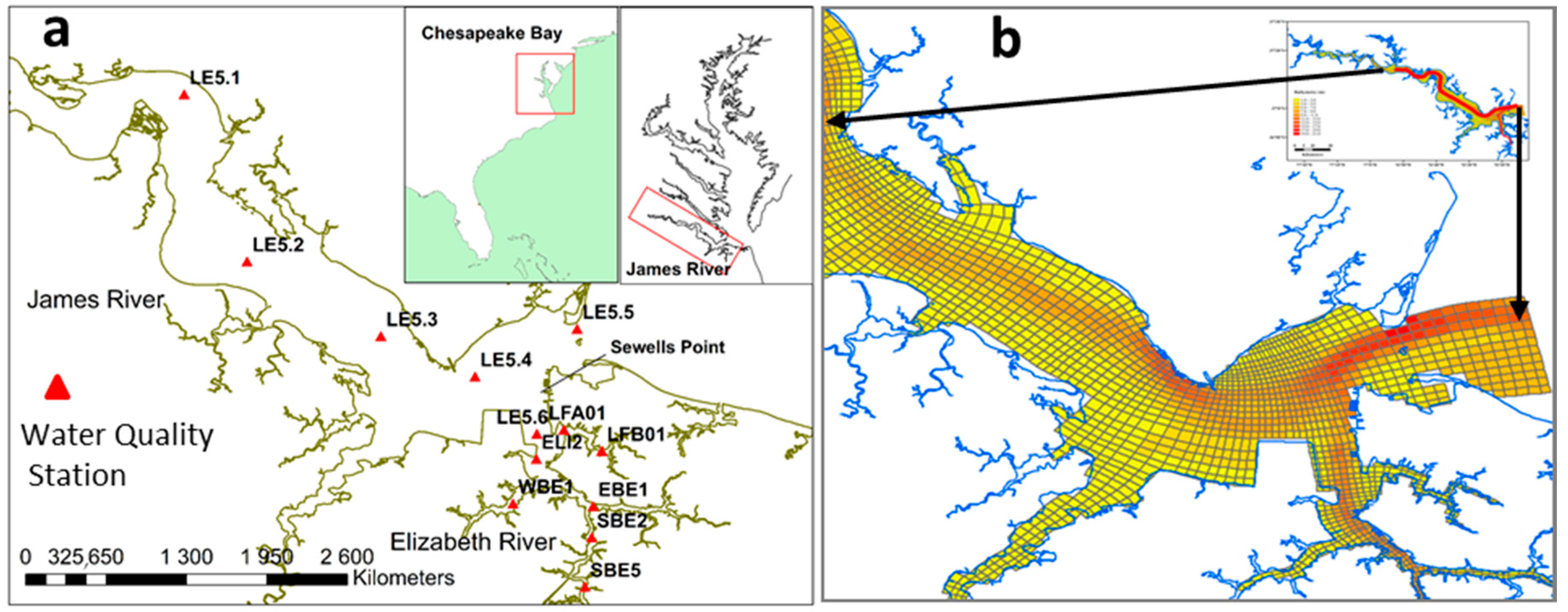
2. Study Area
3. Methods
3.1. Numerical Model
3.2. Transport Time and Bottom Dissolved Oxygen (DO)
3.3. Channel Deepening and Sea-Level Rise Simulations
3.4. Vertical Stratification
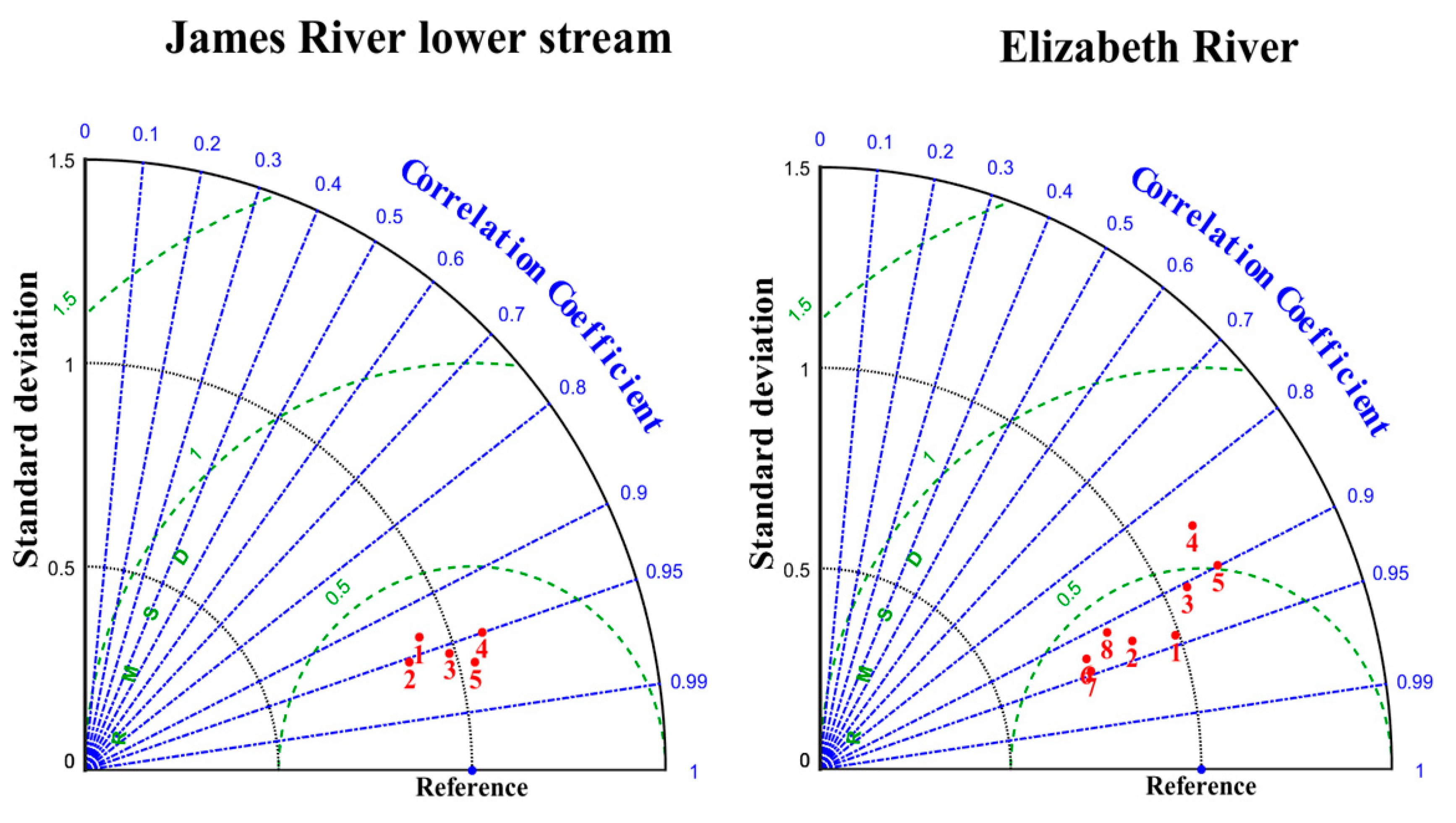
3.5. Model Validation
4. Results
4.1. Change in DO
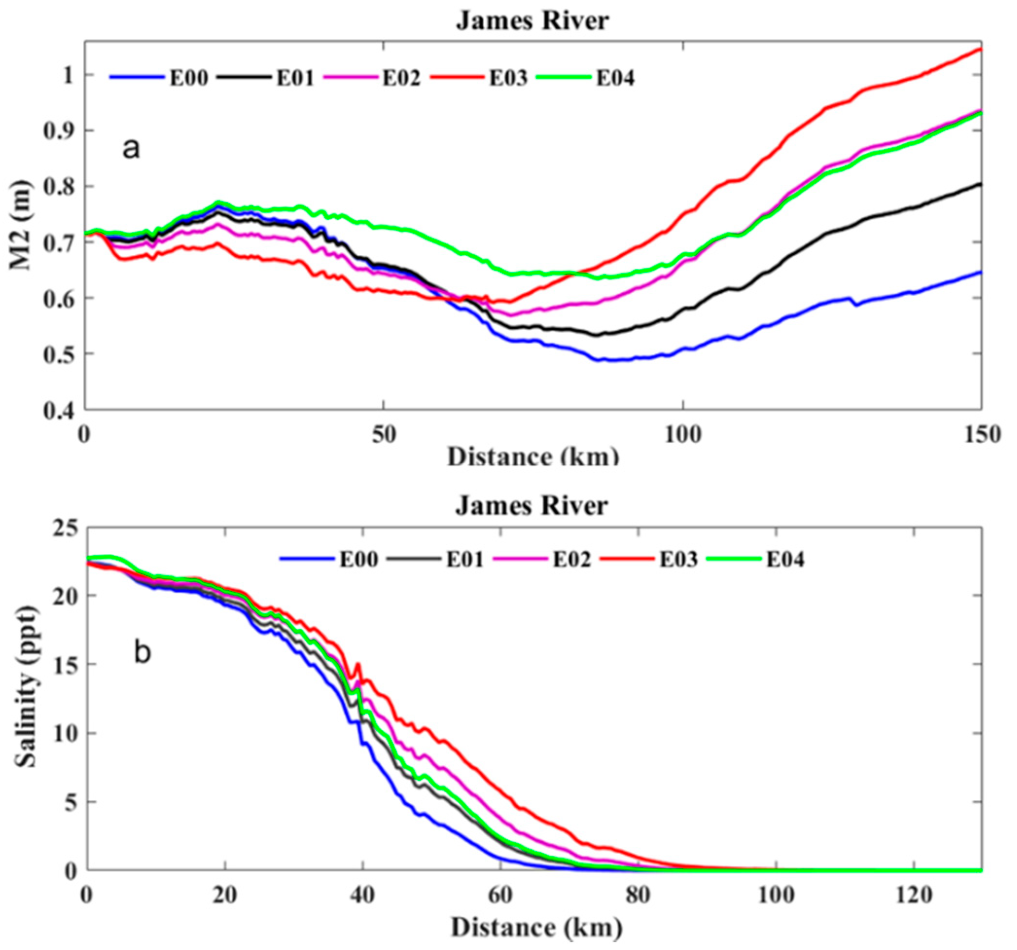
4.2. Change in Tidal Amplitude and Salinity Intrusion
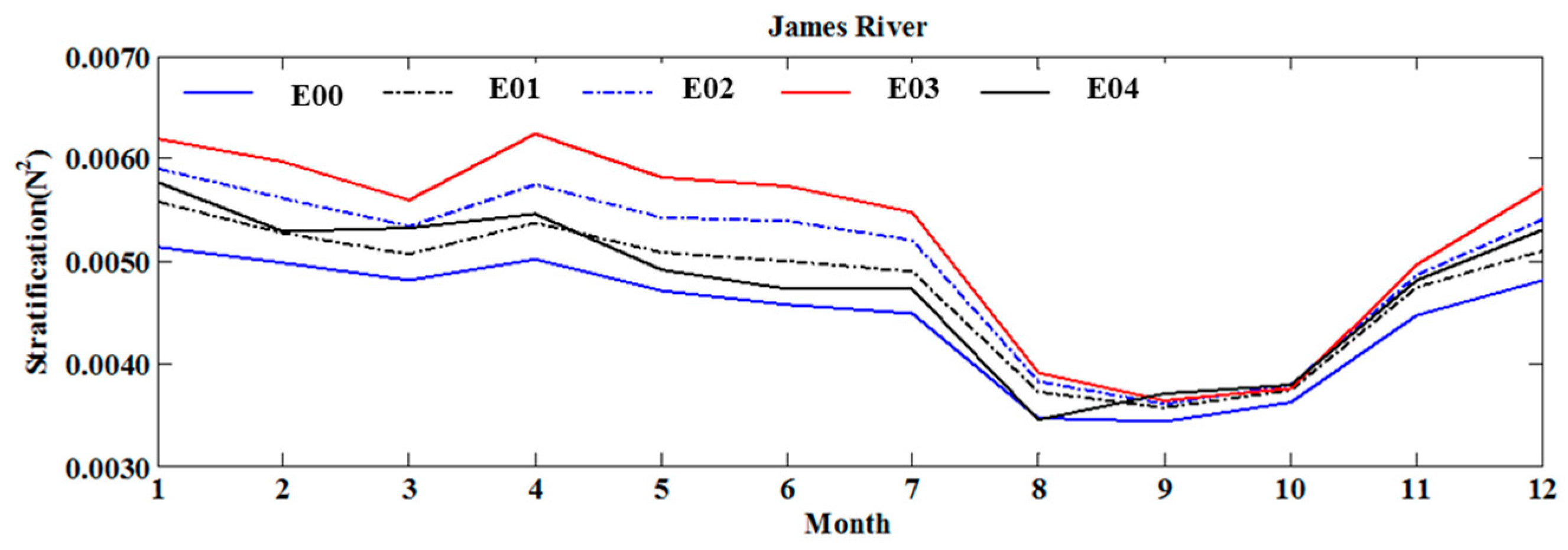
4.3. Change in Stratification
4.4. Change in Gravitational Circulation
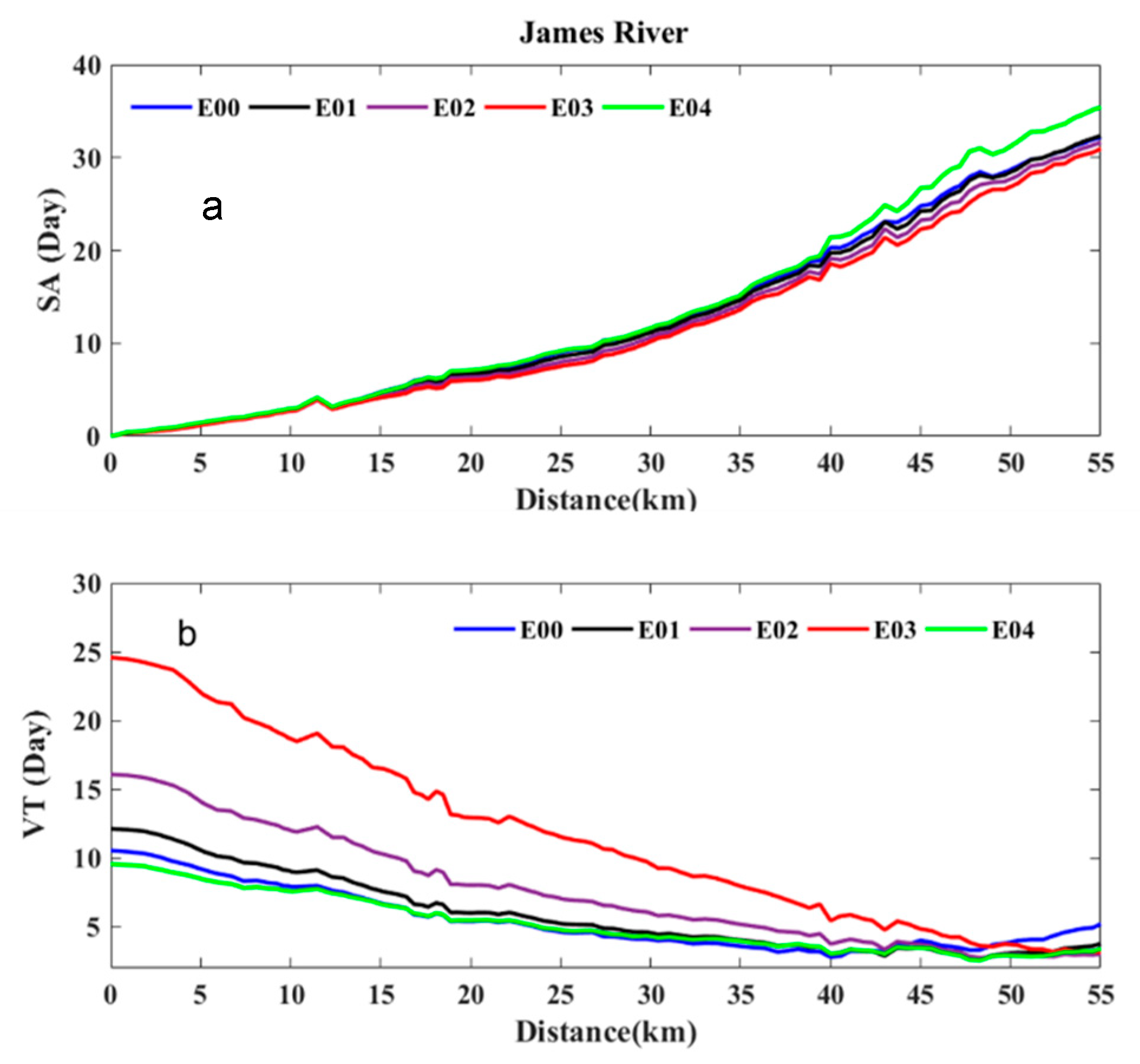
4.5. Change in Saltwater Age along the Transect
4.6. Change in Vertical Exchange Time along Transect
5. Discussion
6. Conclusions
Author Contributions
Funding
Acknowledgments
Conflicts of Interest
References
- Pritchard, D.W. Salinity distribution and circulation in the Chesapeake estuarine system. J. Mar. Res. 1952, 11, 106–123. [Google Scholar]
- Pritchard, D.W. The dynamic structure of a coastal plain estuary. J. Mar. Res. 1956, 15, 33–42. [Google Scholar]
- Familkhalili, R.; Talke, S.A. The effect of channel deepening on tides and storm surge: A case study of Wilmington, NC. Geophys. Res. Lett. 2016, 43, 9138–9147. [Google Scholar] [CrossRef] [Green Version]
- Du, J.; Shen, J.; Zhang, Y.; Ye, F.; Liu, Z.; Wang, Z.; Wang, Y.P.; Yu, X.; Sisson, M.; Wang, H. Tidal response to sea-level rise in different types of estuaries: The importance of length, bathymetry, and geometry. Geophys. Res. Lett. 2018, 45. [Google Scholar] [CrossRef] [Green Version]
- Chant, R.; Talke, S.A.; Sommerfield, C. Impact of Channel Deepening on Tidal and Gravitational Circulation in a2 Highly Engineered Estuarine Basin. Estuaries Coasts 2018, 41, 1587–1600. [Google Scholar] [CrossRef]
- Hansen, D.V.; Rattray, M. Gravitational circulation in straits and estuaries. J. Mar. Res. 1965, 23, 104–122. [Google Scholar]
- Sangita, S.; Satapathy, D.R.; Kar, R.N.; Randa, C.R. Impact of dredging on coastal water quality of Dhammra, Orssa. Indian J. Geo Mar. Sci. 2014, 43, 33–38. [Google Scholar]
- Brown, L.C.; Barnwell, T.O., Jr. The Enhanced Stream Water Quality Models, Qual-2E and Qual-2E UNCAS: Documentation and Users Manual; EPA/600/3-87/007; U.S. Environmental Protection Agency: Athens, GA, USA, 1987. [Google Scholar]
- Kaur, J.; Jaligama, G.; Atkinson, J.F.; DePinto, J.V. Modeling dissolved oxygen in a dredged Lake Erie tributary. J. Great Lakes Res. 2007, 33, 62–82. [Google Scholar] [CrossRef]
- Falkowski, P.G.; Hopkins, T.S.; Walsh, J.J. An analysis of factors affecting oxygen depletion in the New York Bight. J. Mar. Res. 1980, 38, 479–506. [Google Scholar]
- Wang, P.; Linker, L.; Wang, H.; Bhatt, G.; Yactayo, G.; Hinson, K.; Tian, R. Assessing water quality of the Chesapeake Bay by the impact. In Proceedings of the IOP Conference Series: Earth and Environmental Science, 3rd International Conference on Water Resource and Environment (WRE 2017), Qingdao, China, 26–29 June 2017; IOP Publishing Ltd.: Bristol, UK, 2007; Volume 82. [Google Scholar] [CrossRef] [Green Version]
- Irby, I.D.; Friedrichs, M.A.M.; Da, F.; Hinson, K.E. The competing impacts of climate change and nutrient reductions on dissolved oxygen in Chesapeake Bay. Biogeosciences 2018, 15, 2649–2668. [Google Scholar] [CrossRef] [Green Version]
- Kemp, W.M.; Boynton, W.R.; Adolf, J.E.; Boesch, D.F.; Boicourt, W.C.; Brush, G.; Cornwell, J.C.; Fisher, T.R.; Glibert, P.M.; Hagy, J.D. Eutrophication of Chesapeake Bay: Historical trends and ecological interactions. Mar. Ecol. Prog. Ser. 2005, 303, 1–29. [Google Scholar] [CrossRef]
- Cerco, C.; Noel, M. The 2002 Chesapeake Bay Eutrophication Model; EPA 903-R-04-004; US Army Engineer Research and Development Center: Vicksburg, MS, USA, 2004. [Google Scholar]
- Officer, C.B.; Biggs, R.B.; Taft, J.L.; Cronin, L.E.; Tyler, M.A.; Boynton, W.R. Chesapeake Bay anoxia: Origin, development, and significance. Science 1984, 223. [Google Scholar] [CrossRef] [PubMed] [Green Version]
- Kuo, A.Y.; Neilson, B.J. Hypoxia and salinity in Virginia estuaries. Estuaries 1987, 10, 277–283. [Google Scholar] [CrossRef]
- Kuo, A.Y.; Park, K.; Moustafa, M.Z. Spatial and temporal variabilities of hypoxia in the Rappahannock River, Virginia. Estuaries 1991, 14, 113–121. [Google Scholar] [CrossRef]
- Hong, B.; Shen, J. Responses of estuarine salinity and transport processes to potential future sea-level rise in the Chesapeake Bay. Estuar. Coast. Shelf Sci. 2012, 104–105, 33–45. [Google Scholar] [CrossRef]
- Wang, Y.; Shen, J.; He, Q. A numerical model study of the transport timescale and change of estuarine circulation due to waterway constructions in the Changjiang Estuary, China. J. Mar. Syst. 2010, 82, 154–170. [Google Scholar] [CrossRef]
- de Jonge, V.N. Relation between annual dredging activities, suspended matter concentrations, and the development of the tidal regime in the Ems estuary. Can. J. Fish. Aquat. Sci. 1983, 40, 289–300. [Google Scholar] [CrossRef]
- de Jonge, V.N.; Schuttelaars, H.M.; van Beusekom, J.E.E.; Talke, S.A.; de Swart, H.E. The influence of channel deepening on estuarine turbidity levels and dynamics, as exemplified by the Ems estuary. Estuar. Coast. Shelf Sci. 2014, 139, 46–59. [Google Scholar] [CrossRef]
- U.S. Climate Change Science Program. Coastal Sensitivity to Sea-Level Rise: A Focus on the Mid-Atlantic Region. A Report by the U.S. Climate Change Science Program and the Subcommittee on Global Change Research; U.S. Environmental Protection Agency: Washington, DC, USA, 2009; 320p. [Google Scholar]
- Kerner, M. Effects of deepening the Elbe Estuary on sediment regime and water quality. Estuar. Coast. Shelf Sci. 2007, 75, 492–500. [Google Scholar] [CrossRef]
- Zhu, J.; Weisberg, R.H.; Zheng, L.; Han, S. Influences of channel deepening and widening on the tidal and nontidal circulations of Tampa Bay. Estuaries Coasts 2015, 38, 132–150. [Google Scholar] [CrossRef]
- Shen, J.; Hong, B.; Kuo, A.Y. Using timescales to interpret dissolved oxygen distributions in the bottom waters of Chesapeake Bay. Limnol. Oceanogr. Methods 2013, 58, 2237–2248. [Google Scholar] [CrossRef]
- Boynton, W.R.; Kemp, W.M. Nutrient regeneration and oxygen consumption by sediments along an estuarine salinity gradient. Mar. Ecol. Prog. Ser. 1985, 23, 45–55. [Google Scholar] [CrossRef]
- Deleersnijder, E.; Campin, J.M.; Delhez, E.J.M. The concept of age in marine modelling: I. Theory and preliminary model results. J. Mar. Syst. 2001, 28, 229–267. [Google Scholar] [CrossRef] [Green Version]
- Delhez, E.J.M.; Lacroix, G.; Deleersnijder, E. The age as a diagnostic of the dynamics of marine ecosystem models. Ocean Dyn. 2004, 54, 221–231. [Google Scholar] [CrossRef]
- Malone, T.C. Effects of water column processes on dissolved oxygen, nutrients, phytoplankton and zooplankton. In Oxygen Dynamics in the Chesapeake Bay: A Synthesis of Recent Research; Smith, D.E., Leffler, M., Mackiernan, G., Eds.; Maryland Sea Grant College: College Park, MD, USA, 1992; pp. 61–112. [Google Scholar]
- Nixon, S.W.; Ammerman, J.W.; Atkinson, L.P.; Berounsky, V.M.; Billen, G.; Boicourt, W.C.; Boynton, W.R.; Church, T.M.; Ditoro, D.M.; Elmgren, R. The fate of nitrogen and phosphorus at the land-sea margin of the North Atlantic Ocean. Biogeochemistry 1996, 35, 141–180. [Google Scholar] [CrossRef]
- Lucas, L.V.; Thompson, J.K.; Brown, L.R. Why are diverse relationships observed between phytoplankton biomass and transport time? Limnol. Oceanogr. 2009, 54, 381–390. [Google Scholar] [CrossRef]
- Du, J.; Shen, J. Decoupling the influence of biological and physical processes on the dissolved oxygen in the Chesapeake Bay. J. Geophys. Res. Ocean. 2015, 120, 78–93. [Google Scholar] [CrossRef] [Green Version]
- Hong, B.; Shen, J. Linking dynamics of transport timescale and variations of hypoxia in the Chesapeake Bay. J. Geophys. Res. Ocean. 2013, 118, 6017–6029. [Google Scholar] [CrossRef] [Green Version]
- Shen, J.; Wang, Y.; Sisson, M. Development of the hydrodynamic model for long-term simulation of water quality processes of the tidal James River. J. Mar. Sci. Eng. 2016, 4, 82. [Google Scholar] [CrossRef] [Green Version]
- Hamrick, J.M. A Three-Dimensional Environmental Fluid Dynamics Computer Code: Theoretical and Computational Aspects; Special Report in Applied Marine Science and Ocean Engineering. No. 317; Virginia Institute of Marine Science, College of William and Mary: Williamsburg, VA, USA, 1992. [Google Scholar]
- Hamrick, J.M.; Wu, T.S. Computational Design and Optimization of the EFDC/HEM3D Surface Water Hydrodynamic and Eutrophication Models; Society of Industrial and Applied Mathematics: Philadelphia, PA, USA, 1997; pp. 143–161. [Google Scholar]
- Park, K.; Kuo, A.Y.; Shen, J.; Hamrick, J.M. A three-Dimensional Hydrodynamic-Eutrophication Model (HEM-3D): Description of Water Quality and Sediment Process Submodels; Virginia Institute of Marine Science: Gloucester Point, VA, USA, 1995. [Google Scholar]
- Mellor, G.L.; Yamada, T. Development of a turbulence closure model for geophysical fluid problems. Rev. Geophys. Space Phys. 1982, 20, 851–875. [Google Scholar] [CrossRef] [Green Version]
- Galperin, B.; Kantha, L.H.; Rosati, A.; Hassid, S. A quasi-equilibrium turbulent energy model for geophysical flows. J. Atmos. Sci. 1988, 45, 55–62. [Google Scholar] [CrossRef] [Green Version]
- Shen, J.; Qin, Q. James River Water Quality Model Refinement and Scenario Simulations; Special Reports in Applied Marine Science and Ocean Engineering (SRAMSOE) No. 474; Virginia Institute of Marine Science: Gloucester Point, VA, USA; College of William & Mary: Williamsburg, VA, USA, 2020. [Google Scholar] [CrossRef]
- Shen, J.; Haas, L. Calculating age and residence time in the tidal York River using three-dimensional model experiments. Estuar. Coast. Shelf Sci. 2004, 61, 449–461. [Google Scholar] [CrossRef]
- Gustafsson, K.E.; Bendtsen, J. Elucidating the dynamics and mixing agents of a shallow fjord through age tracer modelling. Estuar. Coast. Shelf Sci. 2007, 74, 641–654. [Google Scholar] [CrossRef]
- Rice, K.C.; Hong, B.; Shen, J. Assessment of salinity intrusion in the James and Chickahominy Rivers as a result of simulated sea-level rise in Chesapeake Bay, East Coast, USA. J. Environ. Manag. 2012, 111, 61–69. [Google Scholar] [CrossRef] [PubMed]
- Titus, J.G.; Hudgens, D.E.; Trescott, D.L.; Craghan, M.; Nuckols, W.H.; Hershner, C.H.; Kassakian, J.M.; Linn, C.J.; Merritt, P.G.; McCue, T.M.; et al. State and local governments plan for development of most land vulnerable to rising sea level along the US Atlantic coast. Encviron. Res. Lett. 2009, 4, 4. [Google Scholar] [CrossRef]
- Murphy, R.R.; Kemp, W.M.; Ball, W.P. Long-Term Trends in Chesapeake Bay Seasonal Hypoxia, Stratification, and Nutrient Loading. Estuaries Coasts 2011, 34, 1293–1309. [Google Scholar] [CrossRef]
- Knauss, J.A. Introduction to Physical Oceanography, 2nd ed.; Prentice Hall: Upper Saddle River, NJ, USA, 1997. [Google Scholar]
- Taylor, K.E. Summarizing multiple aspects of model performance in a single diagram. J. Geophys. Res. 2001, 106, 7183–7192. [Google Scholar] [CrossRef]
- Friedrichs, C.T.; Aubrey, D.G. Tidal propagation in strongly convergent channels. J. Geophys. Res. 1994, 99, 3321–3336. [Google Scholar] [CrossRef]
- Scully, M.E.; Geyer, W.R.; Lerczak, J.A. The Influence of Lateral Advection on the Residual Estuarine Circulation: A Numerical Modeling Study of the Hudson River Estuary. J. Phys. Oceanogr. 2009, 39, 107–124. [Google Scholar] [CrossRef] [Green Version]
- Hong, B.; Liu, Z.; Shen, J.; Wu, H.; Gong, W.; Xu, H.; Wang, D. Potential physical impacts of sea-level rise on the Pearl River Estuary, China. J. Mar. Syst. 2019, 201, 103245. [Google Scholar] [CrossRef]
- Bendtsen, J.; Gustafsson, K.E.; Söderkvist, J.; Hansen, J.L.S. Ventilation of bottom water in the North Sea–Baltic Sea transition zone. J. Mar. Syst. 2009, 75, 138–149. [Google Scholar] [CrossRef]
- Boicourt, W.C. The influences of circulation processes on dissolved oxygen in Chesapeake Bay. In Dissolved Oxygen in Chesapeake Bay; Smith, D., Leffler, M., Mackiernan, G., Eds.; Maryland Sea Grant: College Park, MD, USA, 1992; pp. 7–59. [Google Scholar]


| Scenario | Channel Deepening (m) | Boundary Elevation Increase (m) |
|---|---|---|
| E00 | 0 | 0 |
| E01 | 1 | 0 |
| E02 | 2 | 0 |
| E03 | 3 | 0 |
| E04 | 0 | 1 |
| State Variable | ME | AME | RE | RMSE | R |
|---|---|---|---|---|---|
| Chl a (μg/L) | 0.283 | 5.559 | 0.658 | 10.119 | 0.441 |
| NH4 (mg/L) | −0.081 | 0.112 | 0.635 | 0.146 | 0.372 |
| DIN (mg/L) | −0.004 | 0.010 | 0.367 | 0.015 | 0.760 |
| NO2+NO3 (mg/L) | −0.025 | 0.041 | 0.700 | 0.057 | 0.343 |
| PO4 (mg/L) | −0.052 | 0.073 | 0.689 | 0.104 | 0.428 |
| DO (mg/L) | 0.095 | 0.526 | 0.066 | 0.721 | 0.959 |
| Spring | Summer | |||||||||
|---|---|---|---|---|---|---|---|---|---|---|
| Variables | E00 | E01 | E02 | E03 | E04 | E00 | E01 | E02 | E03 | E04 |
| Mean (mg/L) | 7.77 | 7.72 | 7.68 | 7.63 | 7.53 | 6.28 | 6.22 | 6.18 | 6.15 | 6.05 |
| Bottom (mg/L) | 7.66 | 7.58 | 7.53 | 7.46 | 7.37 | 6.11 | 6.01 | 5.95 | 5.89 | 5.81 |
| Mean difference (mg/L) | −0.05 | −0.09 | −0.14 | −0.24 | −0.07 | −0.10 | −0.13 | −0.24 | ||
| Bottom difference (mg/L) | −0.07 | −0.13 | −0.20 | −0.29 | −0.10 | −0.16 | −0.22 | −0.29 | ||
| Relative mean difference (%) | −0.70 | −1.21 | −1.75 | −3.09 | −1.05 | −1.66 | −2.12 | −3.75 | ||
| Relative bottom difference (%) | −0.95 | −1.73 | −2.62 | −3.77 | −1.59 | −2.64 | −3.58 | −4.82 | ||
| Variables | E00 | E01 | E02 | E03 | E04 |
|---|---|---|---|---|---|
| H (m) | 9.38 | 10.35 | 11.33 | 12.31 | 10.38 |
| Salinity gradient (10−4 psu m−1) | 4.62 | 4.31 | 3.91 | 3.52 | 4.35 |
| Eddy viscosity (cm2 s−1) | 32.95 | 30.44 | 28.09 | 27.68 | 30.25 |
| Circulation strength (ms−1) | 0.018 | 0.025 | 0.032 | 0.037 | 0.025 |
Publisher’s Note: MDPI stays neutral with regard to jurisdictional claims in published maps and institutional affiliations. |
© 2020 by the authors. Licensee MDPI, Basel, Switzerland. This article is an open access article distributed under the terms and conditions of the Creative Commons Attribution (CC BY) license (http://creativecommons.org/licenses/by/4.0/).
Share and Cite
Wang, Y.; Shen, J. A Modeling Study on the Influence of Sea-Level Rise and Channel Deepening on Estuarine Circulation and Dissolved Oxygen Levels in the Tidal James River, Virginia, USA. J. Mar. Sci. Eng. 2020, 8, 950. https://doi.org/10.3390/jmse8110950
Wang Y, Shen J. A Modeling Study on the Influence of Sea-Level Rise and Channel Deepening on Estuarine Circulation and Dissolved Oxygen Levels in the Tidal James River, Virginia, USA. Journal of Marine Science and Engineering. 2020; 8(11):950. https://doi.org/10.3390/jmse8110950
Chicago/Turabian StyleWang, Ya, and Jian Shen. 2020. "A Modeling Study on the Influence of Sea-Level Rise and Channel Deepening on Estuarine Circulation and Dissolved Oxygen Levels in the Tidal James River, Virginia, USA" Journal of Marine Science and Engineering 8, no. 11: 950. https://doi.org/10.3390/jmse8110950