Validating UAS-Based Photogrammetry with Traditional Topographic Methods for Surveying Dune Ecosystems in the Spanish Mediterranean Coast

Abstract

In the past few years, unmanned aerial systems (UAS) have achieved great popularity for civil uses. One of the present main uses of these devices is low-cost aerial photogrammetry, being especially useful in coastal environments. In this work, a high-resolution 3D model of a beach section in Guardamar del Segura (Spain) has been produced by employing a low maximum takeoff mass (MTOM) UAS, in combination with the use of structure-from-motion (SfM) techniques. An unprecedented extensive global navigation satellite system (GNSS) survey was simultaneously carried out to statistically validate the model by employing 1238 control points for that purpose. The results show good accuracy, obtaining a vertical root mean square error (RMSE) mean value of 0.121 m and a high point density, close to 30 pt/m², with similar or even higher quality than most coastal surveys performed with classical techniques. UAS technology permits the acquisition of topographic data with low time-consuming surveys at a high temporal frequency. Coastal managers can implement this methodology into their workflow to study the evolution of complex, highly anthropized dune-beach systems such as the one presented in this study, obtaining more accurate surveys at lower costs.

1. Introduction

The coastal dune ecosystems located in arid climate regions represent a unique biotope because of the mutual influence between marine and terrestrial systems. In addition, coastal areas are some of the most popular tourist destinations worldwide. Due to its good climate, together with the great number and length of its beaches, the Spanish Mediterranean coast constitutes one of the most important attractions for domestic and international mass tourism, exploiting the “sun and beach” tourism model [1]. For those reasons, a precise understanding of the beach-dune ecosystems is critical, as they are dynamic areas subject to rapid changes. Apart from natural factors, these ecosystems can be greatly altered by human action, which affects their stability, eventually causing their destruction [2,3].

Dunes in coastal environments are problematic landforms to analyze, owing to the complex interaction among vegetation, topography, aeolian, and marine processes that affect them. For that reason, it is crucial to frequently monitor the terrain to detect dune changes over time in an appropriate way. Traditional surveying methods for obtaining accurate data usually require a large amount of time and labor, even using cutting-edge technologies such as real-time kinematic (RTK) global navigation satellite system (GNSS) surveys [4]. Even though the use of transects might be adequate for modeling a linear and fairly uniform element such as a beach, in a dune area the probability for different transects to correctly represent the behavior of a wider zone decreases dramatically because of the existing horizontal distance between transects [4,5]. Additionally, the reduced resolution of the field data often makes it difficult to obtain accurate volumetric measurements of the dune system.

Emerging terrestrial laser scanning (TLS) technologies offer very accurate infield measurements but they often need to deploy multiple scanning stations throughout the study area due to their limited scanning range and shadow effects caused by obstacles, topography, and vegetation, causing a decrease in performance [6,7]. Moreover, TLS surveys generate an enormous volume of data, which is time-consuming to process, as well as requiring large amounts of storage. Light detection and ranging (LiDAR) systems employed on low altitude flights have been shown to deliver both accurate horizontal and vertical measurements [8]. Various studies have proven the capacity of LiDAR data to represent large coastal areas with sufficient precision (with vertical root mean square (RMS) accuracy values typically ranging from 0.13 to 0.19 m), and its capability to monitor changes over time [9,10,11]. However, it cannot provide data with a comparable spatial resolution and vertical accuracy with respect to TLS and GNSS-based methods. In addition, airborne missions (especially those involving LiDAR) are expensive and complex to organize, so data collection depends in most cases on government-sponsored flights, which reduces or even interrupts their coverage over time [4].

In the present decade, the appearance of affordable low maximum takeoff mass (MTOM) unoccupied aerial systems (UAS) for civil uses, combined with the progress made in modern imagery algorithms, such as structure-from-motion (SfM), has rapidly increased the use of photogrammetric techniques based on UAS to build high-resolution digital surface models (DSM) for studying a wide variety of surface processes [12]. UAS-based photogrammetry provides numerous advantages in contrast with the aforementioned methods. It permits the study of specific zones through fast, high-performance surveys at the desired sample frequency with quality results [13,14].

There are multiple examples of UAS applications in dynamic natural environments: (i) landslide monitoring [15,16,17]; (ii) fluvial dynamics [18,19]; (iii) vegetation monitoring [20,21,22]; or (iv) coastal environment surveying [13,23,24,25,26,27,28].

This investigation is performed on the dune-beach system of Guardamar del Segura coast in Alicante (Spain), where the sustained recession of the shoreline caused by the anthropogenic pressure has severely damaged the dune system and ruined nearby buildings (Figure 1) [29]. The motivation of this work is to assess the feasibility of UAS to undertake periodic precision surveys at much lower costs in the Spanish Mediterranean coast and similar environments by comparing it with classical ground surveying methods, considering the current restrictions existing in these protected zones, as well as national and local UAS regulations [30]. The present study evaluates the applicability of UAS to dune-beach surveys in terms of costs and accuracy. It also analyzes and validates the obtained digital surface model (DSM) with respect to the different types of existing surfaces and contrasts the resulting validation parameters with previous studies made in similar conditions and environments.

For these purposes, a field campaign of flights with a consumer low-cost UAS has been conducted to map the foredune and the adjacent beach. The procedure of UAS image collection and the SfM-based photogrammetric process is described and subsequently analyzed by comparing and validating the results obtained with an unprecedented simultaneous extensive GNSS-based survey involving 77 ground control points (GCP) and 1238 validation points. Results show that UAS is a more precise, faster, and less expensive method than the classical ground surveys. The methodology and results obtained in this work may be useful for studying these valuable areas at risk over time.

2. Materials and Methods

2.1. Area of Study

The study area comprises the coastal area that extends from the north of the town of Guardamar del Segura (Alicante, Spain) to the mouth of the river Segura, belonging to Los Viveros Beach. In particular, it ranges from the shoreline and a nearby pedestrian road for accessing the zone, covering a surface area of 57,000 m², forming a rectangular region with a length of approximately 525 m and a width of 120 m (Figure 2). The prevalent wind directions are ENE and NE, both with a frequency of 15%. A small increase in both frequencies and speeds has been detected in the last decade, with maximum speeds not exceeding 10 m/s. The tidal range is negligible and is only influenced by weather conditions, giving values of approximately 0.3 m [31].

As it is one of the main tourist places in the county, this area is under enormous anthropogenic pressure, not only from the town’s inhabitants, but also from residents of nearby cities and foreign tourists. Additionally, the surrounding urban area recently experienced a strong growth, becoming massively populated, especially during the summer season.

2.2. UAS Field Campaign

The UAS field campaign for data acquisition took place on 12 June 2017, with clear skies and calm periods alternating with weak winds of 2–3 m/s. The equipment used for this study was a low take-off weight UAS model, the DJI Phantom 4 quadcopter (Dà Jiāng Innovations Science and Technology Co. Ltd., Shenzhen, China), valued at $1500 (Figure 3a). This device was equipped with a FC330 built-in camera and a 1/2.3″ CMOS sensor with a maximum resolution of 12.4 Mpixel. The lens has a 94° field of view (FOV), with a 35-mm equivalent focal length of 20 mm and a f/2.8 aperture. It was provided with three 6000 mAh smart batteries that allowed a net flight time of nearly 20 min per battery, totalling one hour per field session. For the mission planning and flight control, the iOS application Pix4D Capture (Pix4D SA, Prilly, Switzerland) was used. The UAS position, status, and the video signal were continuously monitored on the operator screen during the whole flight.

Only two 15-min flights were needed to complete the survey, departing from two different take-off and landing points. The flight path was established in a double mesh layout (longitudinal and latitudinal), permitting redundant overlap of the pictures taken, which is essential for creating a 3D model using SfM algorithms. The flight altitude was set at 60 m above ground level, taking a picture every 2–4 s. The latitudinal overlap was set to 70%, and the longitudinal overlap was fixed to 80%. The average spatial resolution of the images was 2.5 cm/pixel. Two flights were necessary to cover the study area, and a total of 622 images were taken. The flight mission was developed as planned, with no remarkable incidents that could add possible sources of uncertainty.

As the study area is classified as a public domain protected space, it is not allowed to leave any permanent element, including ground control points (GCPs). This fact is even more relevant considering that the zone is frequently crowded during the summer and other holiday periods, making it extremely difficult to keep the permanent GCPs away from people. A total of 77 temporary GCPs were placed before the flight mission and acquired using a Leica Viva GS16 GNSS receiver equipped with real-time kinematic (RTK) positioning technology, used to improve the accuracy of location data acquired from the GNSS (Figure 3a). These points are indispensable for accurately georeferencing the aerial images in the SfM process. Figure 3c shows the target model used for that purpose.

2.3. GNSS Survey

For the purpose of statistically validating vertical and horizontal errors from the UAS survey and to assess the accuracy of the obtained DSM, a total of 1238 complementary GNSS points were surveyed (Figure 4a) in dissimilar characteristic surfaces: dune, beach, road, and wooden walkways. To perform this survey the same Leica Viva GS16 GNSS equipment was used (Figure 4b). This device was linked to the GNSS reference station network of Valencia (ERVA network) via GPRS/3G connection, using RTK with the NTRIP-based network solution to obtain the coordinates in ETRS89 datum. This technology does not consider the distance to the closest station, but the receiver must be inside the area of the triangle defined by the reference stations, as in this case. The accuracy of the acquired data was ±20 mm, both in XY and Z coordinates. The GNSS campaign was carried out the same day as the UAS survey, which involved a 12-h work session, in order to have identical topographic conditions as for the UAS survey.

2.4. SfM-Based Photogrammetry

A photogrammetric procedure based on a SfM algorithm is required for building a high-precision 3D terrain model from the UAS images. Agisoft Photoscan (recently renamed as Agisoft Metashape) Professional Edition software (version 1.2.4, Agisoft LLC, St. Petersburg, Russian Federation) was selected for this work due to its essentially automated workflow, founded on multi-view 3D reconstruction technology, and for its suitability for UAS image processing. Moreover, this software is widely used by researchers worldwide, as it requires little training in SfM photogrammetry, but at the same time offers good quality results. The general workflow for processing the UAS images is divided into seven different steps (Figure 5).

The first step consists of adding images obtained from the UAS, and their camera positions and orientation derived from the UAS sensors, which are contained in the EXIF metadata of the image files. In the next stage, i.e., photo alignment, the software locates tie points among each pair of overlapping images, then adjusts the camera position and orientation for each photo, and eventually builds the sparse point cloud model. The parameters used are shown in Figure 5.

The third step consists of marker placement. Markers are high-precision points distributed throughout the studied area used to optimize camera positions and orientation. This process produces better model reconstruction results and comprises the location of the visible GCPs on each image and the placement of a marker on the corresponding place. The software automatically identifies the position of the markers on every related image, but a manual inspection and a position refinement of the markers is often required to assure good accuracy of the resulting point cloud. For that reason, this stage is usually the most time-consuming one. Lastly, the actual marker coordinates are imported from a file containing the actual coordinates of the GCPs obtained from the GNSS survey.

In the fourth stage of the workflow, camera alignment optimization, the position of the images is recomputed taking into account the previously defined GCPs. PhotoScan settings are established to ensure that the optimization procedure will not consider the camera position given in the images’ EXIF metadata, which is less accurate than that obtained via GCPs. For this purpose, the camera accuracy is set to 10 m and the marker accuracy is 0.001 m, so the resulting point cloud will be georeferenced in terms of XYZ coordinates.

In the next stages, the software calculates the depth map for each camera and combines all of them into a single dense point cloud. The resulting output can be exported as an orthoimage or as a raster DSM, both using the desired coordinate system in a GeoTIFF file format.

SfM techniques demand high computing capability to process and view the resulting models. The technical specifications of the computer used for this task are shown in

Table 1. Technical specifications of the computer used for the photogrammetric process.

Element	Specifications
CPU model	Intel Core i7-2670QM
CPU speed	2.2 GHz
CPU cores/threads	4 cores, 8 threads
CPU internal cache	6 MB
Memory	8 GB DDR3 RAM
GPU	NVIDIA GeForce GT 540M
GPU memory	2 GB DDR3 RAM
Hard disk	Samsung 850 EVO SSD 250 GB
Operating system	Microsoft Windows 10 64-bit

.

3. Results and Discussion

3.1. SfM Process Results

The main parameters resulting from the SfM process are presented in

Table 2. Results of the SfM process.

Parameter	Value
Number of images used	622
Actual flying altitude	61 m
Coverage area	98,600 m2
Number of GCP used	77
GCP RMSE XY	0.089 m
GCP RMSE Z	0.079 m
Dense Cloud Points	2,792,354
DSM Point density	29.6 pt/m2
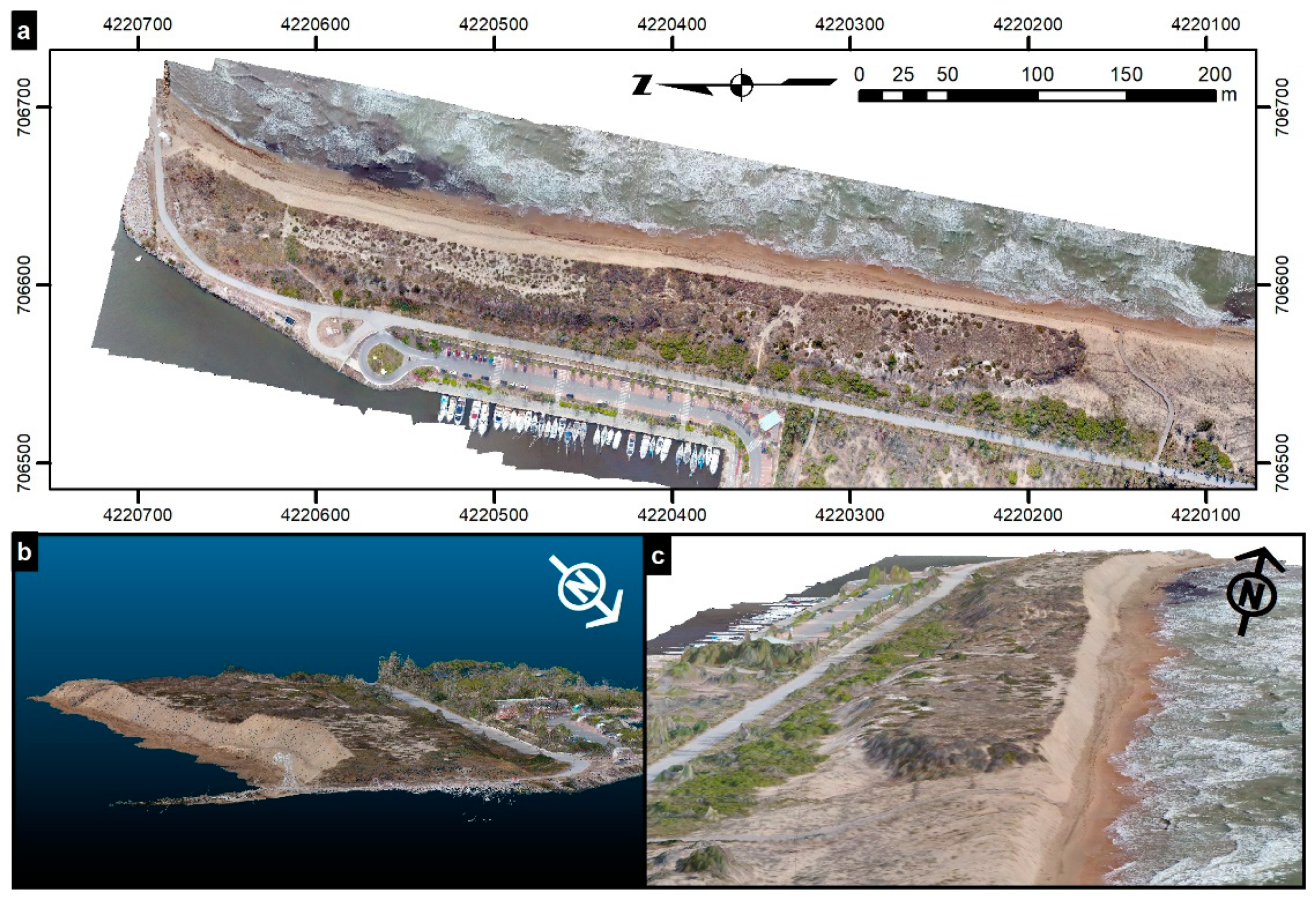
Ground resolution	2.5 cm/pixel

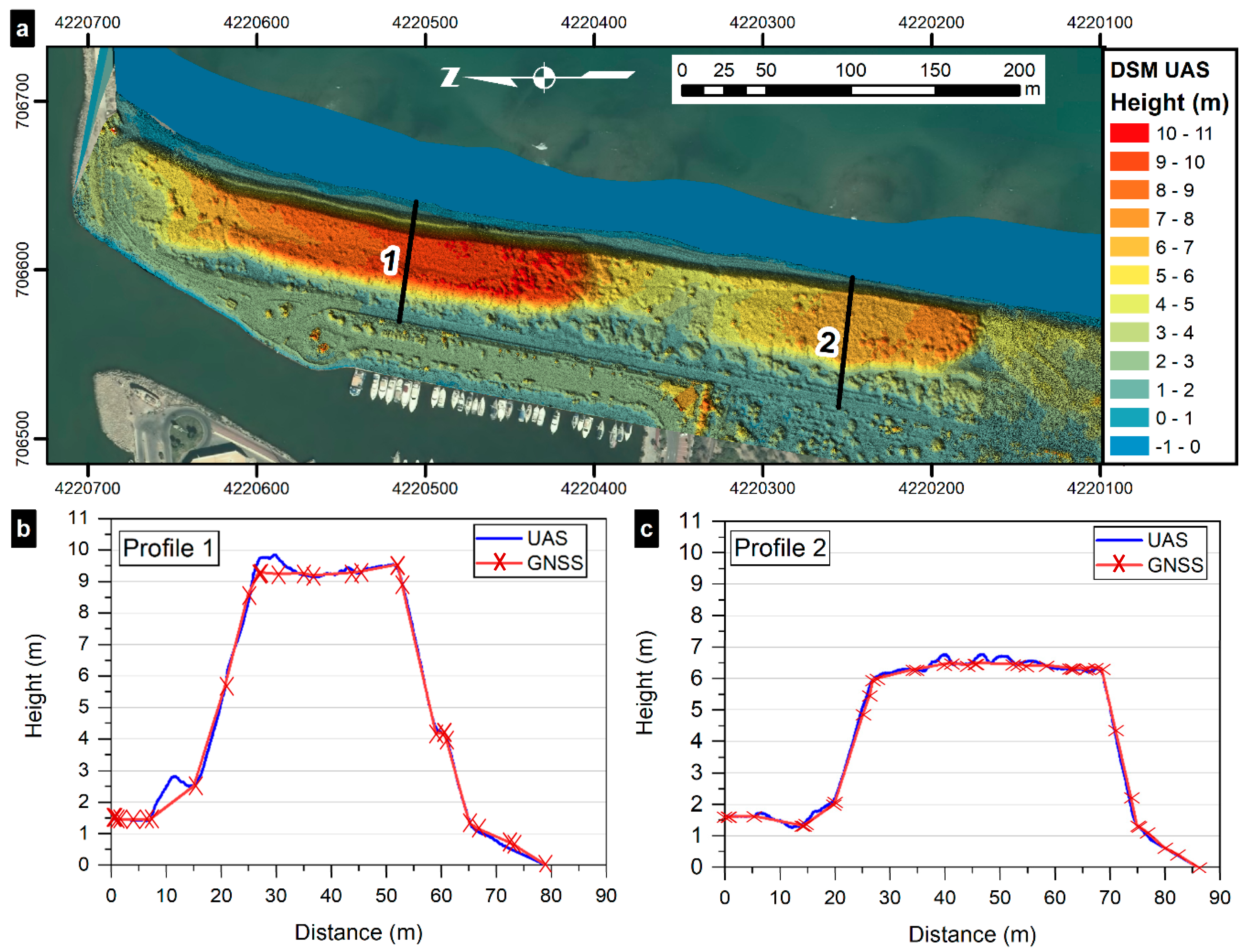
. After processing the images obtained from the two flights, the resulting orthoimage (Figure 6a), the DSM, and the dense point cloud (Figure 6b) were merged into a single dataset for the entire area of study. Almost 2.8 million points form the dense point cloud, which constitutes a three-dimensional model of the surface, with an average density of nearly 30 points per square meter. The digital surface model of the study area was created from the dense point cloud (Figure 6c), with a mean planimetric accuracy of 0.089 m and 0.079 m accuracy for elevation data. The orthoimage created using the UAS imagery and the DSM showed a spatial resolution of 2.5 cm/pixel, precise enough to observe footprints left on sand dunes.

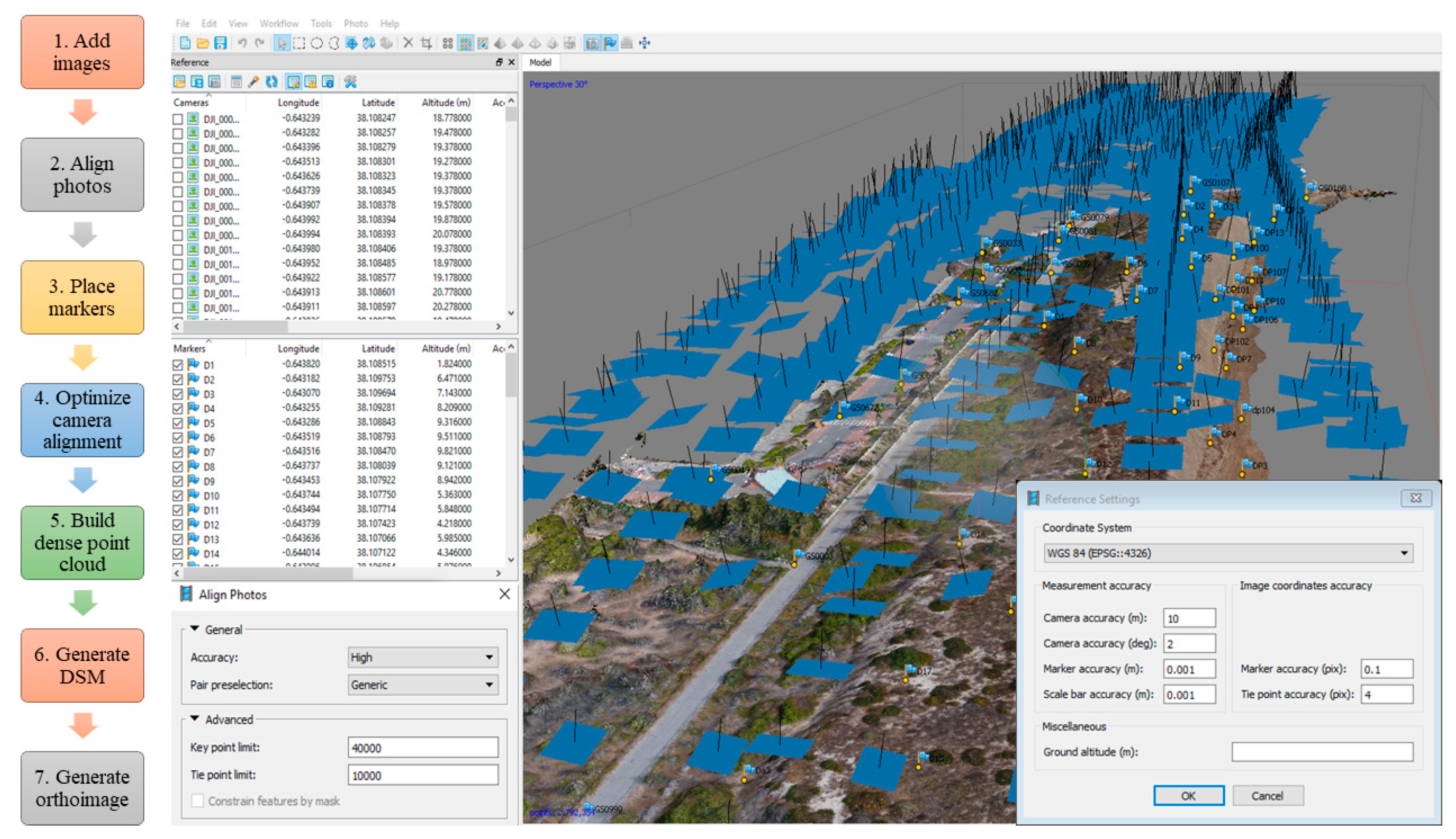
The time elapsed in each stage of the SfM process is displayed in

Table 3. Time performance of the SfM process.

Stage	Processing Time (HH:MM:SS)	Relative Time Consumption (%)
1. Add images	0:00:30	0.1
2. Align images	3:13:00	30.3
3. Place markers	4:45:00	44.7
4. Optimize alignment	0:01:59	0.3
5. Build dense point cloud	2:27:00	23.1
6. Generate DSM	0:05:12	0.8
7. Generate orthophoto	0:04:29	0.7
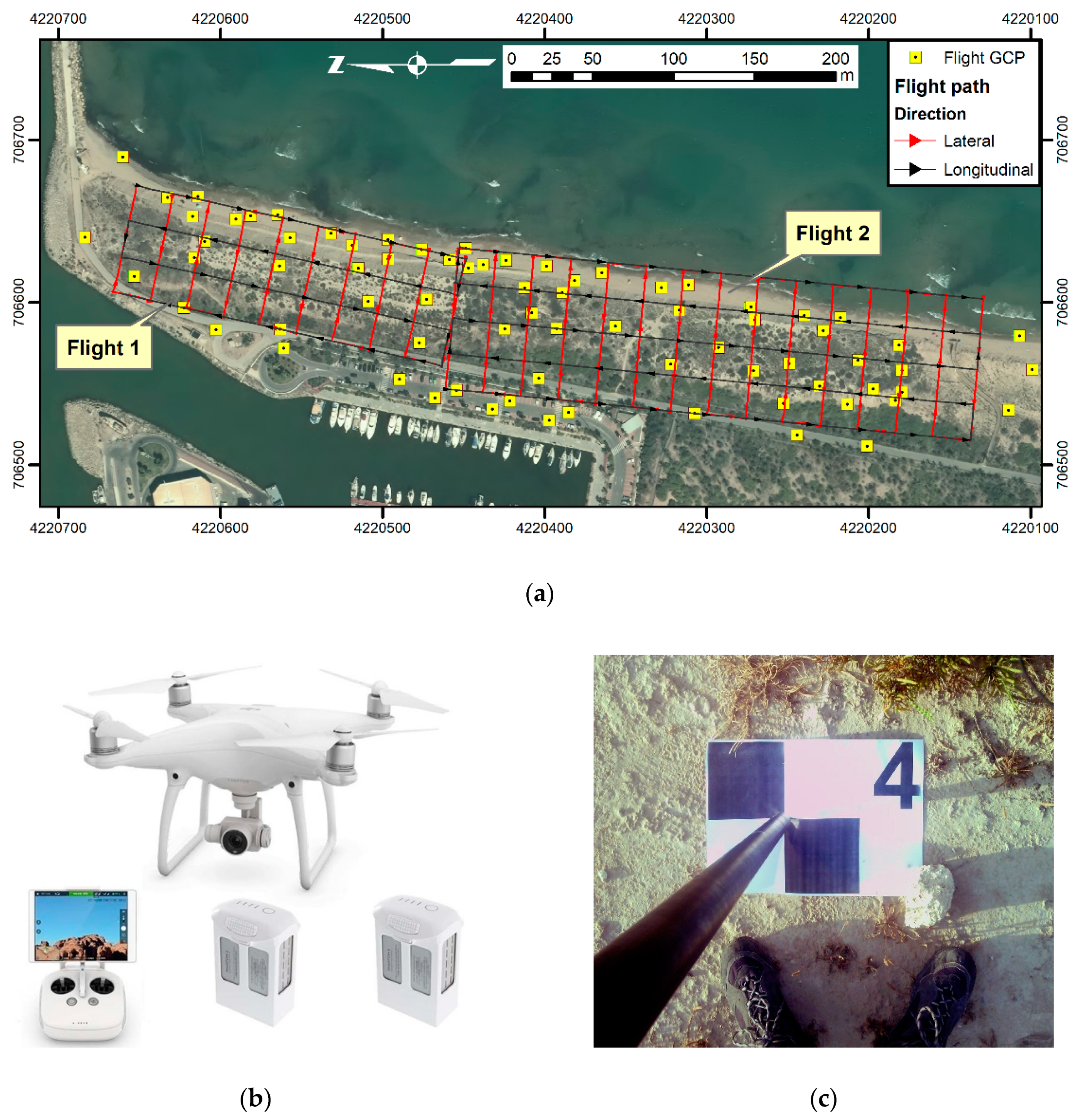
Total time consumed	10:37:10	100.0

. The most time-consuming step was the GCP markers placement, as this task requires human intervention to refine the position of each marker in every image. Because of the high quantity of images and GCPs used (8–12 visible GCPs per image), it took a time span of nearly 5 hours to finalize this phase. The image alignment was the second most time-consuming stage, followed by the dense point cloud generation. Note that these time frames are closely related to the computational power of the computer utilized, so they can be shortened by simply using more powerful computers. The overall time required to complete all the stages of the SfM process was 10 hours and 37 minutes. Nonetheless, in view of the amount of time and labor needed to carry out classical ground surveys, the photogrammetric techniques employed by UAS offer superior performance.

As previously mentioned, dunes are complex surfaces to model, so for this study it was necessary to take such a high number of GCPs. On less complex areas, such as the one described in [14], taking fewer GCPs at the edges and some in the middle of the area of interest (AOI) could be sufficient. However, in this case, apart from the outer edges of the AOI, it was necessary to position targets at both edges of the dune slope (both at the crest and at the dune toe), as well as at the centre of the images. Despite that fact, the processing time could be reduced considering a lesser amount of GCPs per image, considering recent studies in similar zones as the one developed by Laporte-Fauret et al. [32].

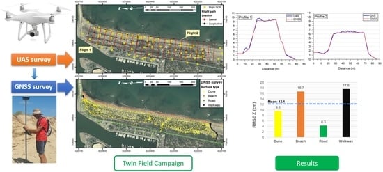
3.2. Validation of the DSM Using the GNSS Survey

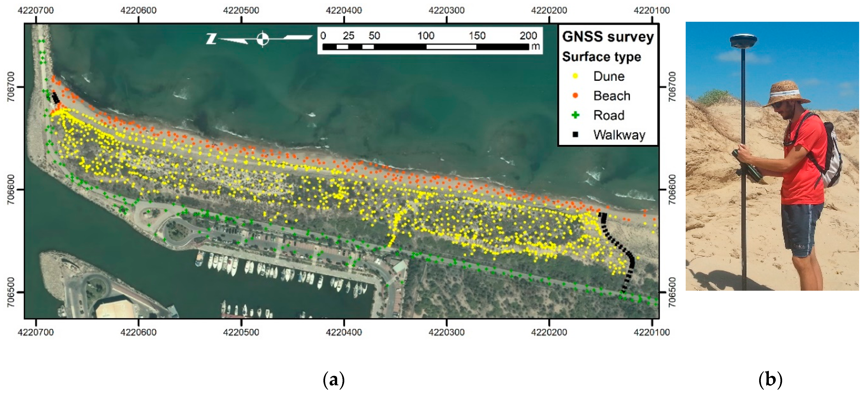
Cross-validation was performed between the measurements taken with the GNSS equipment and those taken from the DSM obtained by means of the UAS survey and SfM processing. For each collected RTK-GNSS point, the elevation of the nearest point from the UAS DSM was extracted. The mean difference (or bias) and RMSE (that is, the standard deviation of the sample) were adopted as measurement error indicators, where positive bias implies that, on average, the UAS exceeded the surveyed elevation using GNSS.

One remarkable contribution from this study is the outstanding number of validation points used in comparison with recent studies carried out in coastal environments, such as the one conducted by Laporte-Fauret et al. using similar image resolution and flight altitude [32]. As the distribution curve of the residuals fits to a normal distribution, the minimum number of validation points n can be obtained using the Equation (1):

$$n={\left(\frac{\sigma }{e}\right)}^2{Z}_{\alpha }^2$$

(1)

where $\sigma$ is the standard deviation of the population, e is the absolute sampling error, and $Z_{\alpha }^{}$ is the normal probability distribution value for the desired confidence level α. In order to obtain a sampling error of 1 cm with a confidence interval of 99% (Z₉₉ = 2.575), the minimum sample size, that is, the minimum number of validation points to survey is:

$$n={\left(\frac{0.121}{0.01}\right)}^2{2.575}^2=971 \mathrm{samples}$$

(2)

As this study has used 1238 validation points, the results presented in this study can be assumed to be statistically representative.

The average value of vertical RMSE was acceptable (0.121 m), with a highly reduced bias of 0.0161 m, indicating a good general accuracy for performing this sort of work in this kind of environments. In fact, previous studies obtained roughly the same RMSE values [13,32,33]. If we compare the obtained RMSE values for the present UAS survey with those achieved using airborne LiDAR surveys [9,10,11], the accuracy is about the same, or even higher.

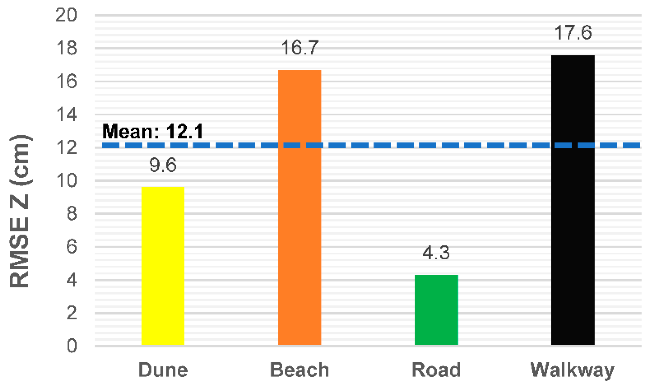
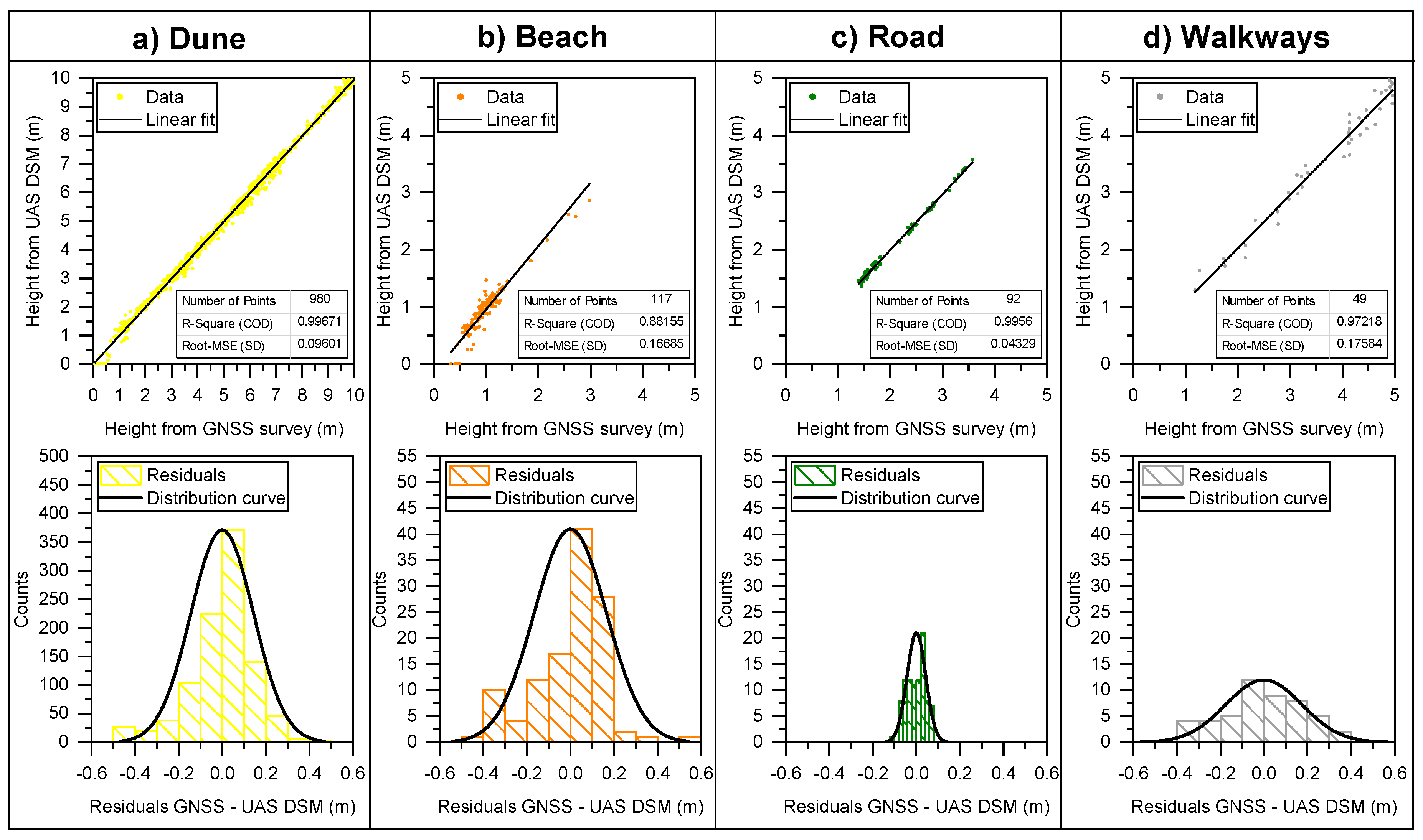
The detailed results of the vertical RMSE obtained for each type of surface are shown in Figure 7. An analysis of the different surface types shows, in general, a good agreement of measurements and a near 1:1 fit between GNSS and UAS data, which means that the accuracy of UAS measurements is equivalent to the obtained GNSS point dataset. The coefficient of determination (COD) values obtained are greater than 0.97 in all of the surface types, except for beach points, where it is close to 0.90. The residuals graphs show similar distribution curves, with mean errors close to zero (Figure 8).

It is commonly accepted that the threshold to determine if a point has been accurately measured or not is that its residuals are below twice the standard deviation (that is, twice of RMSE value).

Table 4. Fit equation parameters and errors (y = a + bx), elevation RMSE, bias, and validation parameters for the different types of surfaces surveyed.

Type of Surface	Dune	Beach	Road	Walkways
Intercept, a	−0.00506 ± 0.01022	−0.15193 ± 0.03978	0.04925 ± 0.0152	0.15714 ± 0.0895
Slope, b	0.99778 ± 0.00183	1.10907 ± 0.03791	0.97409 ± 0.00682	0.93385 ± 0.02304
COD, r2	0.99671	0.88155	0.9956	0.9721
RMSE Z (m)	0.0960	0.1668	0.0433	0.1758
Bias (m)	0.0161	0.0464	0.0059	0.0895
Validation threshold (m)	0.1920	0.3336	0.0866	0.3517
No. of validation points within the validation threshold	827	107	91	48
Number of validation points	980	117	92	49
UAS accuracy (%)	84.4	91.5	98.9	98.0

provides the fit equation parameters, which provide an error correction based on the surface type that other authors can use to quantify DSM uncertainty; for instance, in flood studies, where resolving curbs and pavements can alter flood wave propagation. The table also shows the validation threshold and UAS accuracy values. Overall, 93.2% of the points were accurately measured. In roads and walkways, only one point is over the validation threshold, which means an accuracy of more than 98% (note the variation caused by the different number of points surveyed). The points surveyed in the beach area also have an accuracy of more than 90%. Finally, 84.4% of the 980 points surveyed in the dune area are below the validation threshold, showing a fairly good RMSE Z value of 0.096 m.

However, some differences in accuracy appear when the different surfaces are considered separately. The results show a similar trend to those obtained by Elsner et al. [33]. In this case, DSM data show little systematic differences on the asphalt surface (RMSE Z of 0.043 m), but a more significant divergence on the beach area (RMSE Z mean value of 0.167 m). One of the possible causes that explain that value is the low optical contrast of the beach surface. Homogeneous or reflective surfaces are often problematic for the image matching stage, which leads to a high number of outliers [33]. Surfaces with a heterogeneous and distinct texture are preferred for a more accurate image matching process [34]. The problem of “smooth” surfaces, such as the sand in a beach area, is also highlighted in [35], making them very difficult zones from which to extract highly accurate SfM topographic datasets. This reason might explain the relatively low performance of the UAS-based DSM model when validated using GNSS control points. In the dune zone, however, the presence of shadows cast by the shape of the dune and the existing vegetation helps to increase the heterogeneity of the surface, hence the RMSE value for elevation is considerably lower than on the beach, which is a flat extension of homogeneous sand. The road is a surface with greater contrast than the wooden walkway, the color of which is very similar to the surrounding sand. In consequence, the RMSE Z value in the first surface is lower than in the second case.

Table 5. Comparison between UAS survey parameters for different coastal studies.

Author	Image Resolution (Mpixel)	Mean Flight Altitude (m)	Mean GSD (cm/pixel)	Number of GCP	No. of Validation Points	Bias Z (m)	RMSE Z (m)
Mancini et al. (2013) [13]	18.0	40	0.6	18	126	−0.010	0.11
Gonçalves et al. (2015) [25]	12.0	137	4.7	13	170	0.024	0.062
		131	4.5	13	170	0.035	0.068
		93	3.2	12	148	0.013	0.041
Turner et al. (2016) [27]	18.2	100	3.4	0 (RTK UAS)	15,247	0.026	0.068
Elsner et al. (2018) [33]	16.0	70	1.7	49	1542	−0.053	0.113
					3567	−0.069	0.108
Ruessink et al. (2018) [36]	12.1	Not specified	Not specified	39	147	0.029	0.084
				39	262	0.053	0.107
				33	3191	0.014	0.067
Laporte-Fauret et al. (2019) [32]	12.0	50	4.5	10	65	−0.11	0.13
	20.0		1.78			−0.02	0.05
Bañón et al. (2019)	12.4	61	2.5	77	1238	0.016	0.121
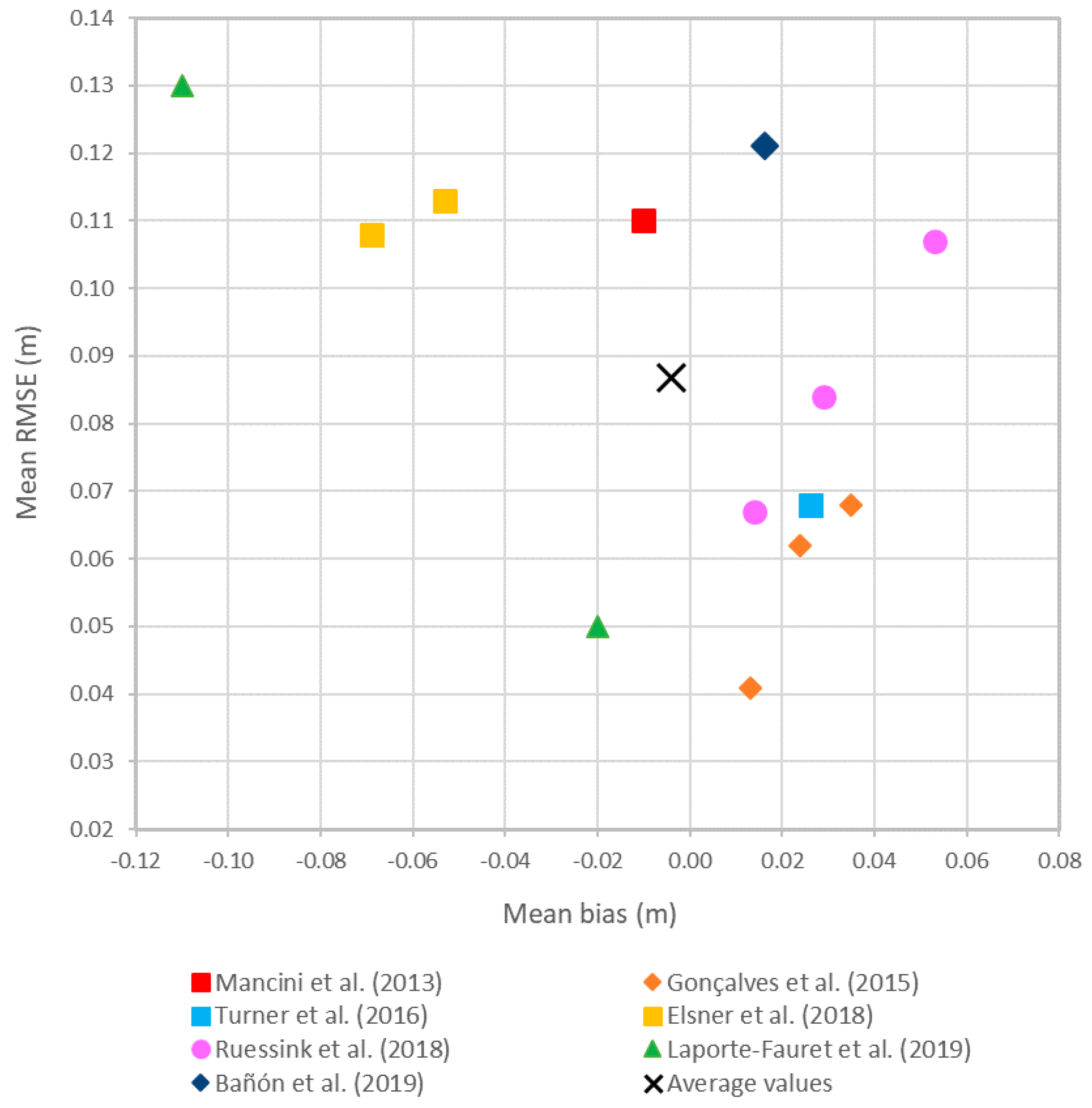
Average value	15.1	85	3.0	30	2156	−0.004	0.087

develops a comparison between previous coastal surveys, indicating the main parameters used for the flight campaign and the vertical accuracy obtained in terms of bias and RMSE. The results show RMSE values ranging from 0.041 m to 0.13 m, with an average value of 0.087, and bias values from ±0.01 to ±0.11, with a mean value very close to zero. Regarding the uncertainty of the GNSS measurements (usually from ±15 to ±20 mm), the different studies show a consistent and similar accuracy, which could be sufficient for surveying this kind of environment.

Figure 9 shows a graphical comparison between the different accuracy values from the studies mentioned in the previous table. It can be seen that the present study comparatively obtains a better value for bias and a higher RMSE value but is very close to some of the analyzed studies. This could be due to the reasons previously described in this article.

3.3. Digital Surface Model and Profile Comparison

Figure 10a shows the DSM obtained from the UAS survey. To check the coherence of the model, two representative profiles of the beach-dune system were selected—one from the north side of the study area and another from the south side. Figure 10b,c shows a comparison of these two profiles using both GNSS and UAS derived datasets. It can be observed that both lines practically overlap. The slight differences shown between the two profiles are caused by the presence of low vegetation, which is difficult to filter with current aerial imaging methods.

A key factor in coastal area monitoring is the determination of the sedimentary budget, which can be used by the coastal or the beach manager to determine which zones of the coast are experiencing regression or transgression processes. For that purpose, it is fundamental to estimate the volume of the sediments, and field surveys are required. To estimate the possible error involved when using UAS-derived data for that task, the cross-section surface area of the two representative profiles has been obtained and presented in

Table 6. Surface area and differences between GNSS and UAS surveys in two representative transects of the study area.

Parameter	Profile 1	Profile 2
UAS surface area (m2)	409.57	357.54
GNSS surface area (m2)	407.77	355.07
Difference UAS-GNSS (m2)	1.80	2.47
Difference UAS-GNSS (%)	0.44	0.70

. It can be easily seen that the margin of error obtained in both profiles is negligible at less than 1%, which validates the UAS methodology hereby explained for performing sedimentary budget estimations with sufficient precision.

3.4. Final Remarks

The novelty in this research is the extensive field survey by GNSS conducted together with the UAS survey. The complexity of the surveyed surface and the homogeneity of the sand may affect the process to create a DSM using the UAS image-based photogrammetry [33,34,35]. For that purpose, 77 GCPs and 1238 validation points were surveyed, a much higher volume than previous recent studies [13,32,33], obtaining statistically sound results. With this wide field survey, this research also outlines the significant reduction in time and costs obtained using UAS and SfM technologies instead of classical GNSS surveys (

Table 7. Time and cost estimations for UAS and GNSS coastal survey methodologies in this study.

Stage	UAS-SfM Methodology		Classical GNSS Methodology
	Time (min)	Cost (USD)	Time (min)	Cost (USD)
Planning and setup	60	40	90	60
Field survey	30	40	720	550
Model generation	637	250	60	150
Total	727	330	900	760

). The surveying time is dramatically reduced from 720 to 30 min, permitting more surface area to be covered within the same session. That is an important factor, especially for extensive zones, such as beaches or dune fields. The model generation time using the SfM methodology could be easily reduced by using less GCPs, as the main time-consuming task is the semi-manual marker placement (see Table 3). Furthermore, the current times and costs will be decreasing rapidly over time as new improvements arrive to the UAS sector.

Nevertheless, there are some disadvantages to consider. Firstly, flight regulations can be restrictive in survey areas, especially near inhabited zones. Particularly, current Spanish regulations for UAS limit their use overcrowded areas without specific permission, such as beaches and over building agglomerations, and the maximum flight altitude is set to 120 m [30]. Secondly, the generated 3D point cloud often includes elevation data coming from undesired sources—buildings, power lines, treetops, and many other elements—instead of from the ground surface, causing a partial distortion of the obtained model. There are several algorithms that mitigate or even correct some of these issues, but they usually demand near infrared (NIR) data to properly detect and filter the vegetation cover [37]. Unfortunately, low-cost UAS are normally not equipped with them.

4. Conclusions

The dune-beach system of Guardamar del Segura has proven to be an exceptional testing site for the methodology presented in the present article. The complex foredune surface and the contiguous beach have been studied using a small, lightweight, inexpensive consumer UAS.

For this study, a twin field campaign was designed, acquiring data from UAS flights and from a GNSS survey. The UAS images were processed through SfM software, obtaining a digital model of the surface. By comparing the two datasets, the results show the high accuracy of UAS-based methodology, obtaining an excellent distribution of residuals and RMSE mean values of 0.12 m, which are similar or even higher than those obtained by employing other techniques, with a good profile fit with the high resolution GNSS terrain model.

Despite the existing minor drawbacks, the advantages of UAS surveys combined with SfM methodology are obvious—a time-saving, consistent, high-precision method that permits the modeling of rapid-changing environments, such as beach-dune systems, at considerably lower costs. Additionally, undertaking periodic and comprehensive surveys to monitor the progression of these complex ecosystems with high reliability and sufficient data quality has been proven possible in this research.

References

1. Palazón, A.; López, I.; Gilart, V.; Bañón, L.; Aragonés, L. Concessions within the maritime-terrestrial public domain on the beaches of southeastern Spain. Ocean Coast. Manag. 2018, 161, 156–164. [Google Scholar] [CrossRef]
2. Bird, E.C.F. Coastline Changes. A Global Review; John Wiley and Sons Inc.: New York, NY, USA, 1985. [Google Scholar]
3. Burak, S.; DoǧAn, E.; GazioǧLu, C. Impact of urbanization and tourism on coastal environment. Ocean Coast. Manag. 2004, 47, 515–527. [Google Scholar] [CrossRef]
4. Andrews, B.D.; Gares, P.A.; Colby, J.D. Techniques for GIS modeling of coastal dunes. Geomorphology 2002, 48, 289–308. [Google Scholar] [CrossRef] [Green Version]
5. Mitasova, H.; Overton, M.; Harmon, R.S. Geospatial analysis of a coastal sand dune field evolution: Jockey’s Ridge, North Carolina. Geomorphology 2005, 72, 204–221. [Google Scholar] [CrossRef]
6. Nagihara, S.; Mulligan, K.R.; Xiong, W. Use of a three-dimensional laser scanner to digitally capture the topography of sand dunes in high spatial resolution. Earth Surf. Proc. Landf. 2004, 29, 391–398. [Google Scholar] [CrossRef]
7. Guisado-Pintado, E.; Jackson, D.W.T.; Rogers, D. 3D mapping efficacy of a drone and terrestrial laser scanner over a temperate beach-dune zone. Geomorphology 2019, 328, 157–172. [Google Scholar] [CrossRef]
8. Woolard, J.W.; Colby, J.D. Spatial characterization, resolution, and volumetric change of coastal dunes using airborne LIDAR: Cape Hatteras, North Carolina. Geomorphology 2002, 48, 269–287. [Google Scholar] [CrossRef] [Green Version]
9. Sallenger, A., Jr.; Krabill, W.; Swift, R.; Brock, J.; List, J.; Hansen, M.; Holman, R.; Manizade, S.; Sontag, J.; Meredith, A. Evaluation of airborne topographic LIDAR for quantifying beach changes. J. Coast. Res. 2003, 19, 125–133. [Google Scholar]
10. White, S.A.; Wang, Y. Utilizing DEMs derived from LIDAR data to analyze morphologic change in the North Carolina coastline. Remote Sens. Environ. 2003, 85, 39–47. [Google Scholar] [CrossRef]
11. Stockdon, H.F.; Doran, K.S.; Sallenger, A.H., Jr. Extraction of lidar-based dune-crest elevations for use in examining the vulnerability of beaches to inundation during hurricanes. J. Coast. Res. 2009, 59–65. [Google Scholar] [CrossRef]
12. Colomina, I.; Molina, P. Unmanned aerial systems for photogrammetry and remote sensing: A review. ISPRS J. Photogramm. Remote Sens. 2014, 92, 79–97. [Google Scholar] [CrossRef] [Green Version]
13. Mancini, F.; Dubbini, M.; Gattelli, M.; Stecchi, F.; Fabbri, S.; Gabbianelli, G. Using Unmanned Aerial Vehicles (UAV) for High-Resolution Reconstruction of Topography: The Structure from Motion Approach on Coastal Environments. Remote Sens. 2013, 5, 6880–6898. [Google Scholar] [CrossRef] [Green Version]
14. Martínez-Carricondo, P.; Agüera-Vega, F.; Carvajal-Ramírez, F.; Mesas-Carrascosa, F.J.; García-Ferrer, A.; Pérez-Porras, F.J. Assessment of UAV-photogrammetric mapping accuracy based on variation of ground control points. Int. J. Appl. Earth Obs. Geoinf. 2018, 72, 1–10. [Google Scholar]
15. Niethammer, U.; James, M.; Rothmund, S.; Travelletti, J.; Joswig, M. UAV-based remote sensing of the Super-Sauze landslide: Evaluation and results. Eng. Geol. 2012, 128, 2–11. [Google Scholar] [CrossRef]
16. Lucieer, A.; Jong, S.M.D.; Turner, D. Mapping landslide displacements using Structure from Motion (SfM) and image correlation of multi-temporal UAV photography. Prog. Phys. Geogr. 2014, 38, 97–116. [Google Scholar] [CrossRef]
17. Huang, H.; Long, J.; Wu, Y.; Yi, Q.; Zhang, G.; Fei, B. A method for using unmanned aerial vehicles for emergency investigation of single geo-hazards and sample applications of this method. Nat. Hazards Earth Syst. Sci. 2017, 17, 1961–1979. [Google Scholar] [CrossRef] [Green Version]
18. Javernick, L.; Brasington, J.; Caruso, B. Modeling the topography of shallow braided rivers using structure-from-motion photogrammetry. Geomorphology 2014, 213, 166–182. [Google Scholar] [CrossRef]
19. Miřijovský, J.; Langhammer, J. Multitemporal monitoring of the morphodynamics of a mid-mountain stream using UAS photogrammetry. Remote Sens. 2015, 7, 8586–8609. [Google Scholar] [CrossRef]
20. Dandois, J.P.; Ellis, E.C. Remote sensing of vegetation structure using computer vision. Remote Sens. 2010, 2, 1157–1176. [Google Scholar] [CrossRef]
21. Jaakkola, A.; Hyyppä, J.; Kukko, A.; Yu, X.; Kaartinen, H.; Lehtomäki, M.; Lin, Y. A low-cost multi-sensoral mobile mapping system and its feasibility for tree measurements. ISPRS J. Photogramm. Remote Sens. 2010, 65, 514–522. [Google Scholar] [CrossRef]
22. Messinger, M.; Asner, G.; Silman, M. Rapid assessments of Amazon forest structure and biomass using small unmanned aerial systems. Remote Sens. 2016, 8, 615. [Google Scholar] [CrossRef]
23. Delacourt, C.; Allemand, P.; Jaud, M.; Grandjean, P.; Deschamps, A.; Ammann, J.; Cuq, V.; Suanez, S. DRELIO: An unmanned helicopter for imaging coastal areas. J. Coast. Res. 2009, Special Issue 56, 1489–1493. [Google Scholar]
24. Drummond, C.D.; Harley, M.D.; Turner, I.L.; A Matheen, A.N.; Glamore, W.C. UAV applications to coastal engineering. In Proceedings of the Australasian Coasts & Ports Conference, Auckland, New Zealand, 15 September 2015; pp. 267–272. [Google Scholar]
25. Gonçalves, J.; Henriques, R. UAV photogrammetry for topographic monitoring of coastal areas. ISPRS J. Photogramm. Remote Sens. 2015, 104, 101–111. [Google Scholar] [CrossRef]
26. Long, N.; Millescamps, B.; Guillot, B.; Pouget, F.; Bertin, X. Monitoring the topography of a dynamic tidal inlet using UAV imagery. Remote Sens. 2016, 8, 387. [Google Scholar] [CrossRef]
27. Turner, I.L.; Harley, M.D.; Drummond, C.D. UAVs for coastal surveying. Coast. Eng. 2016, 114, 19–24. [Google Scholar] [CrossRef]
28. Chen, B.; Yang, Y.; Wen, H.; Ruan, H.; Zhou, Z.; Luo, K.; Zhong, F. High-resolution monitoring of-beach topography and its change using unmanned aerial vehicle imagery. Ocean Coast. Manag. 2018, 160, 103–116. [Google Scholar] [CrossRef]
29. Pagán, J.I.; López, I.; Aragonés, L.; García-Barba, J. The effects of the anthropic actions on the sandy beaches of Guardamar del Segura, Spain. Sci. Total Environ. 2017, 601–602, 1364–1377. [Google Scholar] [CrossRef] [PubMed]
30. Real Decreto 1036/2017, de 15 de Diciembre, Por el Que se Regula la Utilización Civil de Las Aeronaves Pilotadas Por Control Remoto, Ministerio de la Presidencia y Para Las Administraciones Territoriales, Spain. Available online: https://www.seguridadaerea.gob.es/media/4629426/rd_1036_17_rpas.pdf (accessed on 20 July 2019).
31. Estudio Ecocartográfico Del Litoral de las Provincias de Alicante y Valencia. Dirección General de Costas, Ministerio de Medio Ambiente, Spain. Available online: http://www.mapama.gob.es/es/costas/temas/proteccion-costa/ecocartografias/ecocartografia-alicante.aspx (accessed on 20 March 2019).
32. Laporte-Fauret, Q.; Marieu, V.; Castelle, B.; Michalet, R.; Bujan, S.; Rosebery, D. Low-Cost UAV for High-Resolution and Large-Scale Coastal Dune Change Monitoring Using Photogrammetry. J. Mar. Sci. Eng. 2019, 7, 63. [Google Scholar] [CrossRef]
33. Elsner, P.; Dornbusch, U.; Thomas, I.; Amos, D.; Bovington, J.; Horn, D. Coincident beach surveys using UAS, vehicle mounted and airborne laser scanner: Point cloud inter-comparison and effects of surface type heterogeneity on elevation accuracies. Remote Sens. Environ. 2018, 208, 15–26. [Google Scholar] [CrossRef]
34. Baltsavias, E. A comparision between photogrammetry and laser scanning. ISPRS J. Photogramm. Remote Sens. 1999, 54, 83–94. [Google Scholar] [CrossRef]
35. Fonstad, M.A.; Dietrich, J.T.; Courville, B.C.; Jensen, J.L.; Carbonneau, P.E. Topographic structure from motion: A new development in photogrammetric measurement. Earth Surf. Process. Landf. 2013, 38, 421–430. [Google Scholar] [CrossRef]
36. Ruessink, B.; Arens, S.; Kuipers, M.; Donker, J. Coastal dune dynamics in response to excavated foredune notches. Aeolian Res. 2018, 31, 3–17. [Google Scholar] [CrossRef]
37. Kyratzis, A.C.; Skarlatos, D.P.; Menexes, G.C.; Vamvakousis, V.F.; Katsiotis, A. Assessment of Vegetation Indices Derived by UAV Imagery for Durum Wheat Phenotyping under a Water Limited and Heat Stressed Mediterranean Environment. Front. Plant Sci. 2017, 8, 1114. [Google Scholar] [CrossRef] [PubMed]
Figure 1. Effects of the shoreline recession on nearby buildings, caused by anthropogenic stress: (a) shoreline in 2008; (b) same view in 2017.
Jmse 07 00297 g001
Figure 2. (a) Location of the province of Alicante, southeast Spain; (b) location of the town of Guardamar del Segura within the province of Alicante; (c) location of the study area with respect to the town; (d) aerial image of Segura river mouth, Los Viveros beach, and the perimeter of the study area, outlined in red.
Jmse 07 00297 g002
Figure 3. (a) Flight plan performed and location of the surveyed GCPs; (b) DJI Phantom 4 equipment used for image acquisition; (c) GCP targets used.
Jmse 07 00297 g003
Figure 4. (a) Location of GNSS survey points; (b) co-author performing the GNSS survey in the study area.
Jmse 07 00297 g004
Figure 5. Workflow followed for SfM modelling (left); a snapshot of Agisoft Photoscan software, showing the position of the images, photo alignment, and camera settings, the location of GCPs, and the dense point cloud finally obtained (right).
Jmse 07 00297 g005
Figure 6. (a) Orthoimage from UAS; (b) 3D dense point cloud; (c) 3D view of the dune derived from the orthoimage and DSM surveyed by the UAS.
Jmse 07 00297 g006
Figure 7. Vertical RMSE per surface type.
Jmse 07 00297 g007
Figure 8. Linear fit and residual analysis of the generated DSM model according to the surface type: (a) dune; (b) beach; (c) road; (d) walkways.
Jmse 07 00297 g008
Figure 9. Mean accuracy values obtained by different authors in coastal surveys.
Jmse 07 00297 g009
Figure 10. (a) Digital surface model (DSM) from UAS images. (b) Profile 1 surveyed by GNSS and derived from UAS DSM. (c) Profile 2 surveyed by GNSS and derived from UAS DSM.
Jmse 07 00297 g010