Video Sensing of Nearshore Bathymetry Evolution with Error Estimate

Abstract

Although coastal morphology results essentially from underwater sediment transports, the evolution of underwater beach profiles along the diverse coastlines of the world is still poorly documented. Bathymetry inversion from shore-based video cameras set forth a more systematic evaluation and is becoming more commonly used. However, there are limitations to this profiling method that are insufficiently assessed, undermining confidence in operational applications. In this paper, we investigate the daily evolution of a low tide terrace (LTT) in Nha Trang beach, Vietnam, under strong seasonal forcing: from weak wind waves during summer monsoon to moderate waves during winter monsoon. A new error estimation for depth inversion is presented based on tidal evaluation. The method compares video-based estimate and direct measurement of tidal amplitudes to provide a quality criterion. It reveals three types of errors, the main one being a deep water error associated with physical limits—loss of celerity-bathymetry relationship in deep water. This error is dependent on wave period and thus has a strong seasonal pattern in Vietnam. It is generally detrimental to depth inversion where wind waves are dominant (in summer here). On the contrary, the second error type is larger for larger waves and is located at breakpoint, altering wave detection. The last error type is due to nonlinear effects and wave setup in shallow water. After removing the faulty data, we finally present the first reliable three-year time-series of a beach profile in Nha Trang, Vietnam. A main result is the overall stability demonstrated for the LTT beach, with rapid exchange of sediment between the terrace and the upper beach during typhoons, monsoon events or seasonal cycles. These tropical environments may provide faster beach recovery compared with mid-latitude configurations.

Highlights

• New method of depth-inversion error estimate using tides
• Guidelines on the limits of video-based depth inversion
• Three-year analysis of low tide terrace evolution from video cameras

1. Introduction

Low tide terrace (LTT) beaches are a common type of sandy beach but is one of the least documented [1]. It can be seen both in low-tide (microtidal) [2,3] and high-tide (macro- and meso-tidal) regimes [4,5]. While the flat lower terrace area is generally alongshore-uniform, the steeper upper part often presents rhythmic cusps [6]. The terrace formation is due to a coupling process between the effects of tides and waves. At low tide, waves plunge heavily on the outer terrace, but at high tide, they may pass across the terrace unbroken to surge up the beach face, producing reflection [7,8,9]. LTT are intermediate beaches associated with low incoming wave energy [4,10]; theoretically, it can transform into a transverse bar and rip state (TBR) when wave energy increases and into the lowest energy beach state, which is a reflective beach, when energy decreases. LTT beaches commonly features weak waves and coarse sand.

After more than 30 years of development, many coastal studies produced results using video systems, including for long-term morphological evolution [11,12]. However, most are limited to the description of shoreline or submerged-bar location because these are possible in all conditions. Beach profiling from bathymetry inversion is another challenge, and is not commonly tackled even though it is in high demand. Image quality has several sources of error: validity of modulation transfer function (link between surface elevation and optical signal, see [13]), breakpoint discontinuities, wave conditions, weather (lighting), geometrical conditions. Automated extraction techniques are thus known to produce high noise levels [14] that can make geometrical interpretation difficult. If first-rate data is beyond reach, we need at least to estimate their quality. Recent results from cBathy—an inversion method using a Kalman filter [15]—show that the methodological error can be estimated directly from video techniques [16]. However, other error types are due to physical assumptions used in depth inversion. Inversion relies on the linear wave theory that provides a dispersion relation between wave propagation and bathymetry for shallow and intermediate depths. Even though a few studies produce video-based bathymetry estimates—from drones [17,18] or shore-based cameras (e.g., [14,19])—little attention is assigned to error estimates, even though the method is often applied from very shallow to deep waters, without much consideration to the theory’s validity.

Quantifying beach morphodynamics requires monitoring beach profiles on a wide range of timescales. Conventional measurement techniques have obvious limitations because they are time consuming, costly and hazardous. These disadvantages do not apply to remote techniques such as shore-based video systems and LiDAR or satellite imagery [20,21]. Continuous video monitoring now reveals the beach response to wave forcing at different timescales [16,22]. In particular, video-based estimation of shoreline position is now rather straightforward, which makes it possible, for example, to estimate the timescales of beach recovery after a storm—about nine days in Biscarrosse (southwest France) [23], and three days in Nha Trang, central Vietnam [24,25]. But by considering only the shoreline, these studies do not take into account the evolution of the beach profile. For the reasons discussed above, high-frequency (i.e., daily) estimates of beach profiles are subject to high noise levels that are often simply filtered. For example, [26] produce a dataset covering more than three years but its time resolution is limited to seven days after averaging over the tidal cycle and removing poor-quality data due to lighting issues (e.g., sun glint). This makes it difficult to study short-term events. But even at seasonal scale, the validity of video-based depth inversion during a low-energy season is not demonstrated.

In the present study, we present the three-year morphological evolution of a low tide terrace sandy beach in Nha Trang, Vietnam, based on bathymetry inversion from a shore-based camera system. Special care is given to the validity range of data inversion and removal of faulty data based on a new method for error estimate. Then, an analysis of morphodynamics is given at different scales from seasonal to short-term events. The results show that the width of a low tide terrace is an important parameter of beach evolution. The discussion section finally provides guidelines on the limits of video-based inversion for future applications in the diverse coastlines of the world.

2. Methods

2.1. Study Area

Nha Trang beach is a sandy beach located in a semi-closed bay in the south of Vietnam (Figure 1). This bay of about 6 km is oriented north–south, facing the fetch limited South China Sea. A group of islands located in the southeast corner of the bay partially shelters it from short to moderate southeast wind waves during summer monsoon. During winter monsoon, however, Nha Trang bay is exposed to long, high-energy northwest longer waves [24,25,27,28]. The offshore annual mean significant wave height $H_s$ is 0.95 m, with an associated averaged peak period $T_p$ of 6.2 s. Waves show seasonal variability: during fall and winter seasons (October to April), mean $H_s$ is 1.2 m and $T_p$ is 6.8 s, while during spring and summer (May to September) mean $H_s$ is reduced to 0.6 m with a shorter $T_p$ below 5 s. Waves generally hit this sheltered embayed beach with near shore-normal incidence. Nha Trang bay experiences mixed diurnal and semi-diurnal tides [25,27] with a micro-tidal range from 0.4 m to a maximum of 1.7 m.

Several extensive in-situ surveys were conducted between 2013 and 2016 (26–30 May 2013; 3–10 December 2013; 12–19 June 2015; 28 November–3 December 2015; and 20–24 December 2016), along with more than three years of video monitoring. This dataset revealed the characteristics of Nha Trang beach as a low tide terrace sandy beach with a steep upper beach face (slope ∼ 0.1) and a narrow, alongshore-uniform, flat terrace of slope ∼ 0.01 and width 10–40 m [25,27]. The mean sediment size varies significantly within the bay, with coarse sand in the North ($D_{50}=0.9$ mm) reducing to medium-to-coarse in the South ($D_{50}=0.4$ mm) [27,29]. Based on three years of 15-min image analyses of the shoreline [25], the beach state of Nha Trang beach did not appear to change from year to year. During high-energy conditions beach cusps and mini-rips occurred but the shoreline rapidly straightened after less than three days. The submerged beach was not analyzed in these studies.

Figure 1 presents the configuration of Nha Trang bay and the beach profiling location (cross-shore transect) in the central part of the bay where cross-shore time-stack images are created for depth inversion.

2.2. Video Data

A shore-based video system [30,31,32] was installed in May 2013 in the central part of Nha Trang bay by researchers of Thuy Loi University in collaboration with LEGOS/IRD-France [24,25,28,33,34]. The video station contains two color cameras (VIVOTEK IP7361, max-resolution 1600 × 1200 pixels) fixed on an existing light pole nearby, located 70 m from shore and at 14.3 m above mean sea level (MSL). The power of the system was supplied by the post office. The camera recorded data at a frequency of two frames per second stored first in an internal memory card. The raw video data was then downloaded through Internet connection to a server at Thuy Loi University. From the raw images, three types of secondary images were created every 15 min (snapshots, cross-shore time-stacks, and 15 min time exposure images). A total of 931 days of data, from 25 May 2013 to 27 August 2016, were used for analysis. Rectification of images from pixel to real world coordinates is accomplished by direct linear transformation using 59 RTK-GPS ground control points [35] after correction for the lens radial and tangential distortions [36]. With some variation over the field of view, the pixel footprint for cross-shore and alongshore directions is about 0.25 m and 0.05 m, respectively, in the region of interest (surfzone of the instrumented zone). Time-stack images are interpolated on a regular grid using MSL reference and parameters obtained in the rectification step, with the native time resolution (2 Hz) and a regular space resolution of 0.5 m. The error in celerity caused by floating pixel-position is considered negligible. This is especially true for micro-tidal environments such as Nha Trang beach but probably less for meso- to macro-tidal environments [15]. Tidal data was obtained at Cau Da station at the southern end of the bay. The offshore wave field was extracted from ERA-Interim global reanalysis provided by the European Centre for Medium-Range Weather Forecasts (resolution of $0.5^{\circ }$ and six-hourly; Dee et al. [37]) at the closest node off Nha Trang. This assimilated model product was validated over a two-month period using a local wave gauge [25]. Land and sea morphological surveys were conducted over the study period, and are also used in this study to validate video estimates.

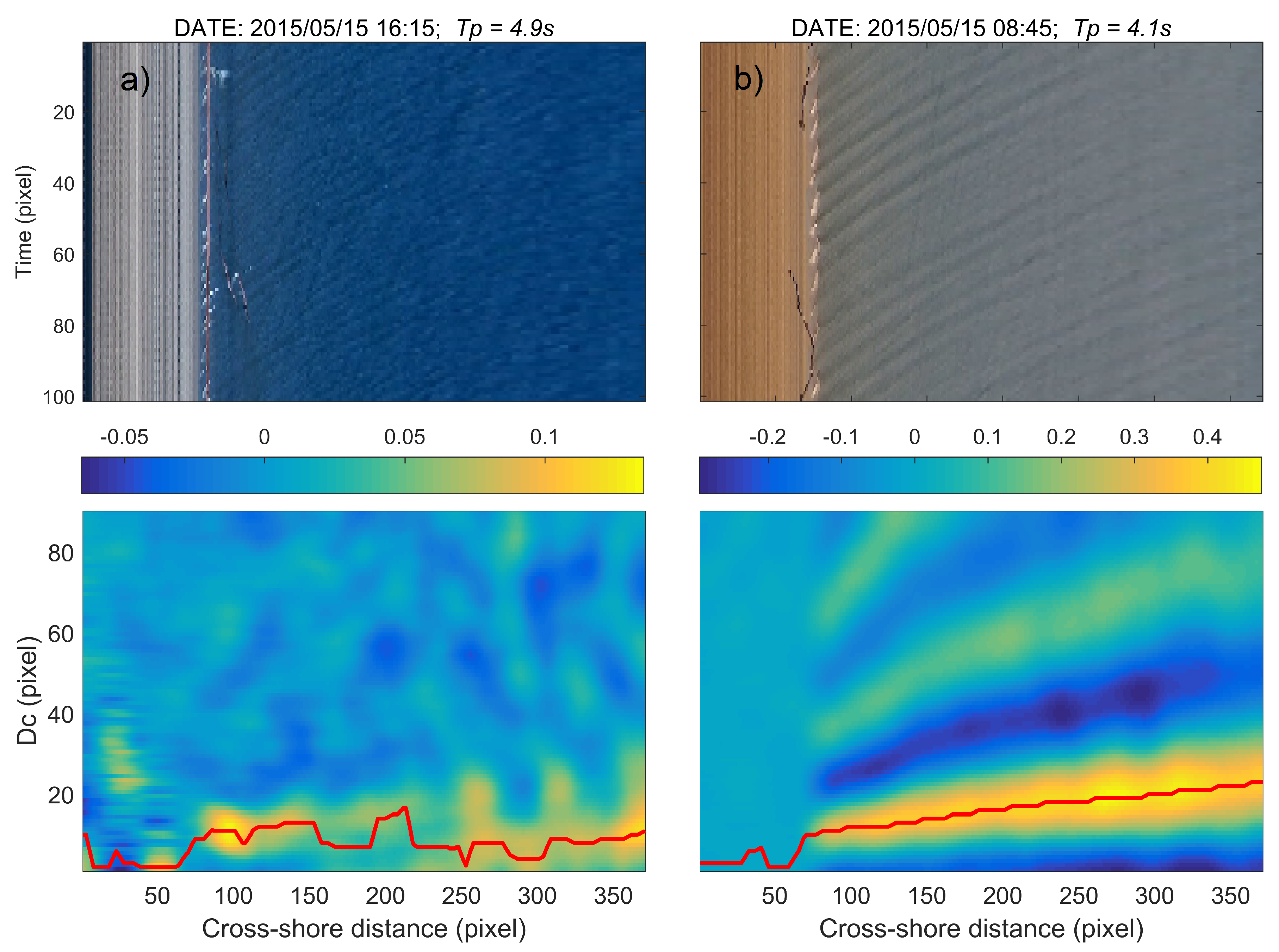
2.3. Depth Inversion along a Cross-Shore Transect

Two different approaches for depth inversion are generally applied in near-shore camera systems [19]. The spectral method of cBathy is two-dimensional while the cross-correlation temporal method used in this study is one-dimensional [38,39]. The latter is adapted to the acquisition strategy at the Nha Trang site, which was designed to save on storage capacity for long-term monitoring purpose, only storing relevant information along a few cross-shore transects. [19] show that the two methods give similar results with similar entry data, although applying a one-dimensional method to a cross-shore transect can be an issue for an oblique wave incidence angle and can affect the depth estimate. However, this issue is minor in our case of an embayed beach with near shore-normal incident waves [40]. The incident wave direction does not significantly affect the accuracy of wave celerity determination and we estimate that for a wave angle less than 15 deg, the error is less than 3.5%.

First, cross-shore timestack images are pre-processed to improve the wave intensity signal. A pass-band filter between 0.05 and 0.5 Hz is used to remove low-frequency (light variations due to clouds) and high-frequency components (rapid adjustment of the camera “auto-iris”). Then, the signal is normalized by dividing the intensity wave signal with the local intensity maximum [38].

Second, a temporal cross-correlation method [16,38,39] is applied to invert time stack images for water depth. This method derives wave celerity from temporal cross-correlations. At each location X, a correlation is computed between time series of neighbor locations $\Delta X$, adding a time lag $\Delta \varphi$ to neighbor time series. A matrix of resulting correlation coefficients M is obtained as a function of X and $\Delta X$:

$$M(X,\Delta X)=cor\left(\eta \right(X,t),\eta (X+\Delta X,t+\Delta \varphi \left)\right).$$

(1)

The maximum correlation value of M for a selected range of $\Delta X$ gives the average distance $\Delta X_0$ made by the waves within $\Delta \varphi$ at each location X. This can be converted to a celerity C:

$$C=\frac{\Delta X_0}{\Delta \varphi }.$$

(2)

The use of a time lag $\Delta \varphi$ is preferred to a direct cross-correlation, which gives the wavelength L for an associated period T, then $C=L/T$. This is motivated by a better spatial resolution ($C\Delta \varphi$ instead of L) that allows resolving smaller-scale bathymetric features. $\Delta \varphi$ must be chosen less than or equal to T. $\Delta \varphi =3$ s is a reasonable value for most wave conditions. The depth is finally derived from the linear dispersion relation for free surface waves using the video-derived wave celerity C and wave period T [19,39].

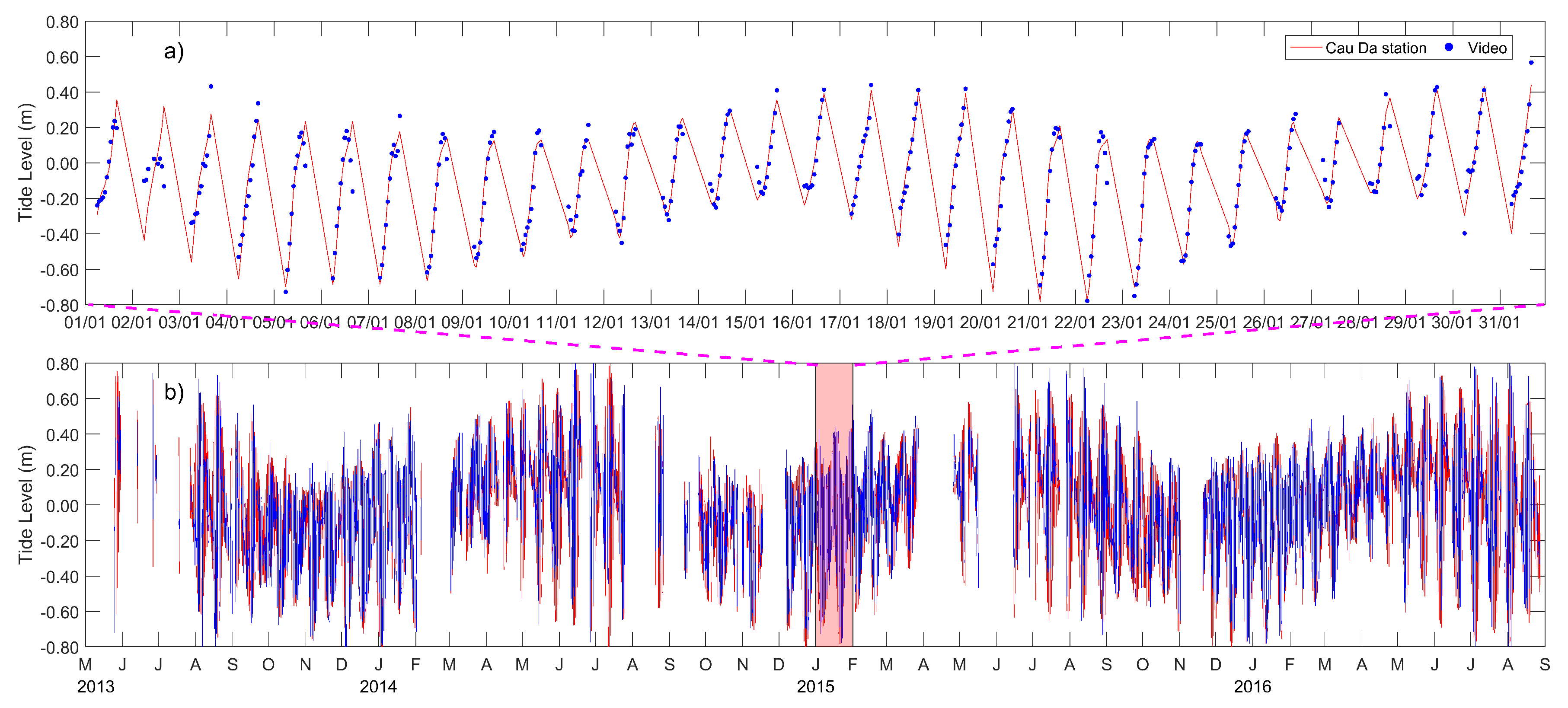
2.4. Using Tide as a Quality Proxy

As discussed in the introduction, a major challenge for depth inversion is to assess the validity of the method associated with methodological and physical induced errors on bathymetry estimate, which varies with wave and tide conditions. A rational approach is needed to identify erroneous data and extract a useful dataset. Here, we propose a novel way to quantify the quality of daily data based on the availability of a local tidal gauge located a few hundreds of meters away from the camera in Nha Trang bay.

Figure 2 shows an example of image analysis for the morning of 15 May 2015 with no-wind waves and afternoon with windy choppy waves, where short wave conditions prevailed. The morning presents clean (easily detectable wave crests) wave conditions on the cross-shore time stack image, leading to a smooth cross-correlation matrix and straightforward celerity estimation. The afternoon presents more sea-breeze choppy conditions with local wind waves perturbing the sea state to the point where the cross-correlation matrix cannot be of any use. Higher frequency cameras could improve the detection of wave propagation from that image but correcting noise level is not sufficient for proper depth inversion. The problem is deep water limitation (see the “Discussion” section) as the waves here are too short to interact with the sea bed, unless they get very close to shore. As a result, both morning and afternoon images are unfit for depth inversion, independently of noise level. To cope with the physical validity of depth inversion and more generally with any sources of error, we designed a simple method.

Assuming little morphological evolution during one day, any variability of water depth within this day can be associated with tides. In this case, the video-based depth estimate D can be split into a daily averaged component, i.e., the bathymetry h varying with sediment transport according to the Exner equation1 , and an anomaly $\eta$ varying with tides:

$$D=h+\eta .$$

(3)

We extracted the video-based tidal signal $\eta$ as a time anomaly of the inverted depth:

$$\eta =D-\overline{D},$$

(4)

where $\overline{D}$ is a three-day moving average of D, assumed to equal h. The extracted tidal signal from depth inversion is shown in Figure 3 together with tidal gauge measurement. Ref. [39] recently evaluated sea level from video inversion at Grand Popo Beach (Benin, West Africa), but did not use it to construct a simple error estimator, which is our present proposition. For the tide gauge time series, we also remove a three-day moving average, similarly to the video data, for consistent removal of atmospheric effects on sea level (inverse barometer and Ekman drift). The comparison with tidal measurements in Figure 3 shows generally good agreement, particularly in winter and away from breakpoint and very shallow waters (the three error types that will be discussed in more details later). For error estimation, we compute the root mean squared errors (RMSE) between video and tide gauge measurements of high-frequency (tidal) sea level for each day in the time-series. The good days are assumed to be those with RMSE less than 0.2 m. Daily error on bathymetry is then estimated based on these tidal differences between tide gauge observation and video-based inversion. We will come back to the error estimate in more details in the Discussion section.

3. Analysis of Beach Profile Evolution

Here, we present a beach profile analysis for Nha Trang during the three year measurement period. We will focus on the terrace width and its evolution at seasonal scale and as a response to intense winter monsoon events. As explained in the previous section, data quality control is essentially provided by the error estimate based on tides. But some comparison with bathymetry surveys were also done for validation. The example of Figure 4 during the NT4 survey of fall 2016 shows that error seems to increase with distance to shore but the main aspect of the profile, i.e., the terrace, is captured by the inversion method (more discussion on the error in Section 4).

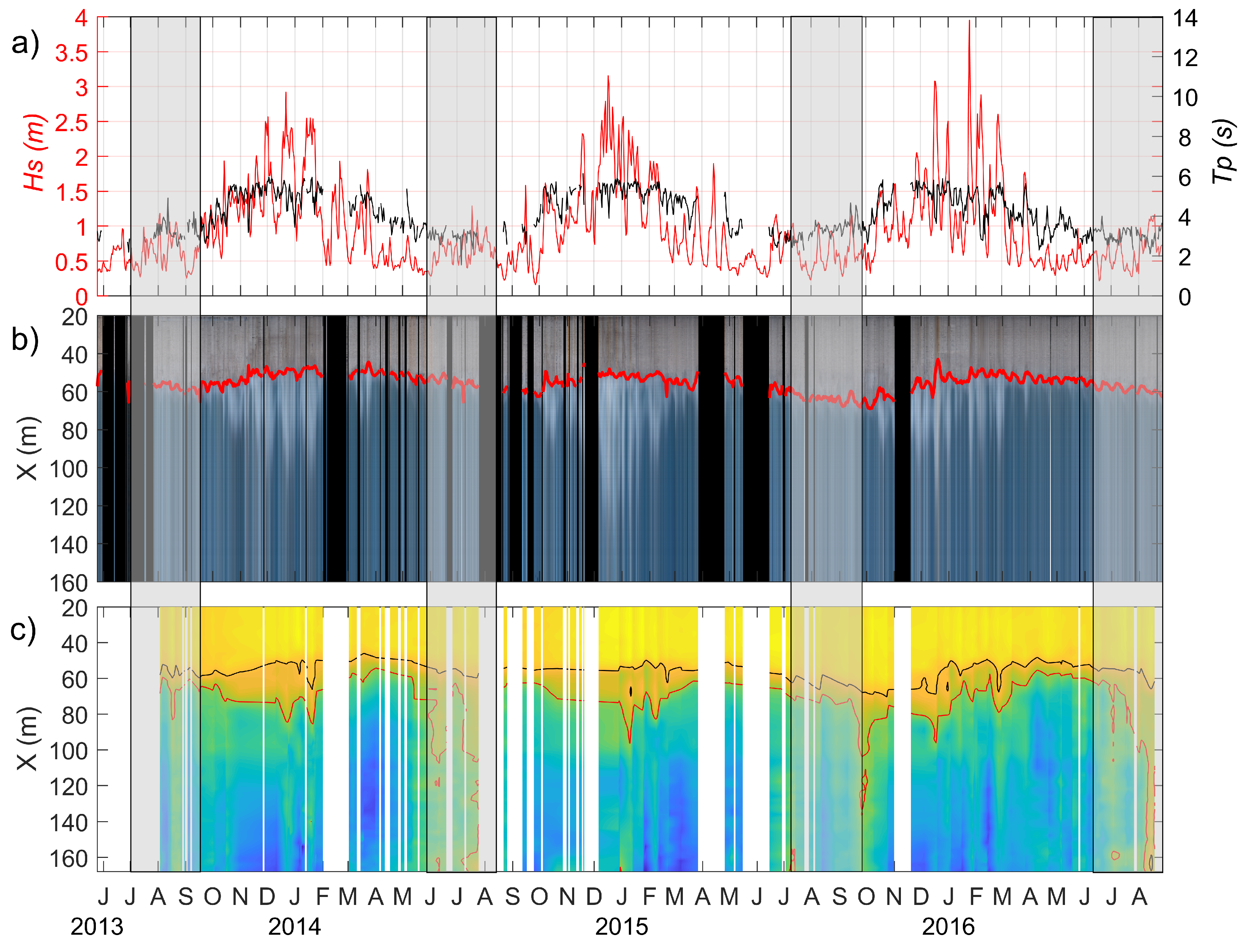
3.1. Bathymetry Evolution

Figure 5a shows off-shore wave forcing and beach response over the 3.5 years of the study period for the profiling location presented in Figure 1.

Wave forcing exhibits variability at multiple scales. Wave height $H_s$ is provided by ERA-Interim while the average period $T_m$ (zero-crossing) is derived from the video images and thus better accounts for local waves. The seasonal scale clearly stands out with high-energy northeast moderate waves during winter monsoon (October to April; $H_s=1.7$ m, $T_p=6$ s) and small local wind waves during summer monsoon (May to September; $H_s=0.5$ m, $T_p=3$ s). Interannual variability is also present but largely as a result of intrinsic variability of strong winter monsoon events (three days to three weeks; $H_s=3$ m) that largely imprints the signal in winter. Short-term events (<3 days) are associated with typhoon landing but their imprint is more sporadic (from October to December essentially) and not considerably stronger than monsoon events.

Daily mean cross-shore time stack video images are shown in Figure 5b. This allows us to visualize and understand the evolution of shoreline position. This has been analyzed in detail in [25] and the results will be summarized in the following for interpretation of beach profile evolution. Figure 5c shows the daily cross-shore video-derived beach profile, where the low tide terrace area is indicated. This low tide terrace shows a significant variability at short event (during the winter season) and seasonal scales. In the following, we concentrate on the response of the terrace to seasonal and monsoon events.

3.2. Seasonal Pattern

Figure 6 shows wave forcing and beach response over a mean annual period over the 3.5 years of the study and a low-pass filter reveals seasonal patterns (moving average with a window of 30 days). Unfortunately, during summer, the amount of “good” bathymetry data is too small to allow any reliable observation (see Discussion). Nevertheless, the end and beginning of winter monsoon (with decreasing and increasing wave energy—see Figure 5a) provides useful information on the transition to summer period, so that a sense of seasonal evolution can be determined. Shoreline evolution—which is available all year long—can help completing the picture on beach evolution.

From February to the end of the summer monsoon in October, the shoreline position is stable at first, then accretes more rapidly. In September, it begins an erosive phase due to winter monsoon conditions until February when it reaches its most landward location, 10 m from its summer position [25].

The terrace follows an opposite behavior, with a terrace width becoming narrower with decreasing wave energy and wider with increasing energy. There is thus good correlation at the seasonal scale between the evolution of wave energy, shoreline and terrace width. From September to December, when wave energy increases, the shoreline erodes at the same time that the terrace expands. Then, from January to April, wave energy decreases while the shoreline begins its recovery and the terrace width decreases from 18 m (January) to 9 m (April). Interestingly, the speed of terrace evolution is much faster in this period than that of shoreline recovery, which is maximum in summer. This can be explained by different sediment fluxes during the periods of increasing and decreasing wave energy. During increasing energy, the terrace expands at the expense of the shore face, while during the decreasing energy, the terrace appears to loose sand to the offshore slope as much as to the shore face.

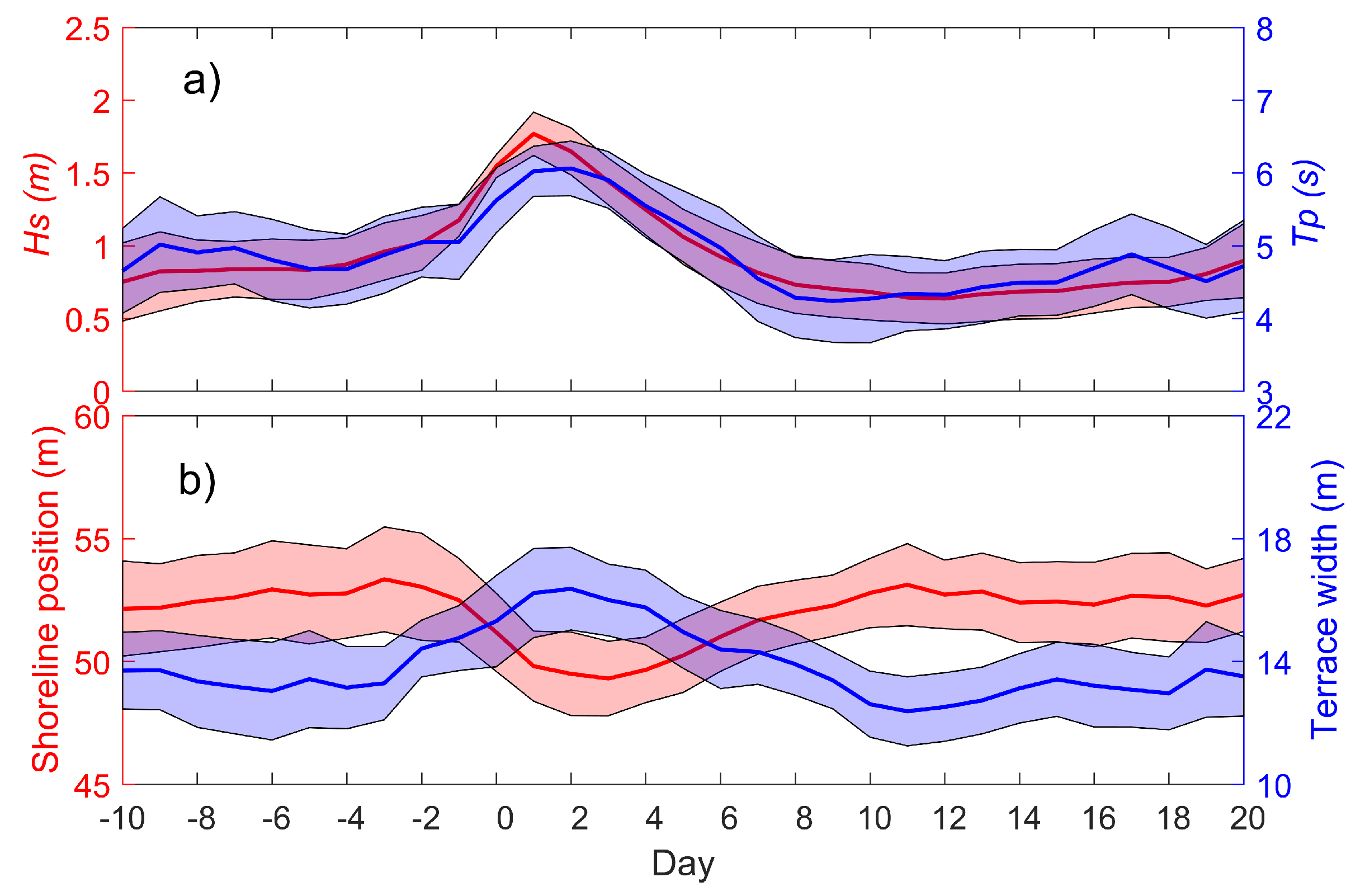
3.3. Impact of Winter Monsoon Events

Besides a strong seasonal cycle, the coast of Vietnam is largely impacted by intense winter monsoon events that last from three days to three weeks [25]. Typhoon events are also present but they are less numerous and of shorter duration (see next section). To identify the events, the Peak Over Threshold method (POT) [1,23,41,42] was applied on the offshore significant wave height ($H_s$) provided by ERA-Interim. The 2% exceedence threshold was used to identify strong events. Then, to characterize their general impact, we construct a composite beach profile as an ensemble mean of all events, thereby providing statistical reliability. Note that the composite hides some of the variability associated with winter monsoon events. For example, shoreline variations can reach 10 m during the strongest winter events but only half of that remains in the composite. Figure 7 presents the composite event for the periods before and after occurrence (day 0): wave forcing (wave height and period), shoreline position, and terrace width.

Day 0 for each event is defined as the time when wave height crosses a given threshold that must be high enough to be considered an event. For that reason, the composite event appears to start a bit earlier around day −2. The wave height rises during three days from the onset of the event where it reaches a peak value of a bit less than 2 m. At the same time, the period rises as well, indicating the presence of longer waves that has developed across the South China Sea. The wave height and period then slowly reduces over about a week.

As waves pick up the shoreline quickly retreats about 4 m in 3–4 days and then slowly recovers in about nine days. The terrace width follows a very similar pattern, but with a negative relationship. It first rapidly increases about 4 m following the rise of wave height and then slowly recovers as waves decline. The average post-event beach recovery duration is thus about 9 days both for the shoreline and terrace (i.e., whole beach profile accretion). Clearly, shoreline erosion is a process that provides sand to the terrace and inversely, shoreline accretion feeds on the terrace during recovery. The low tide terrace is thus the sand reservoir of the beach and is easily accessible for wave-induced onshore transport to nourish the upper beach.

3.4. LTT Beach State Dynamics and Recovery

Interestingly, while the beach shoreface adapts to changing wave conditions, it never changes its state as a low tide terrace. For example, transition to a barred beach could be expected during high energy conditions, but does not seem to occur. This suggests that LTT beaches are a stable type and can handle a large variety of waves and tides. One of the most striking properties of LTT is its rapid response time (days typically). This can be attributed to the fast exchange of sediment between the upper beach part and the terrace. It can be compared to a barred beach, which typically exhibits a response time larger than 10 days [23], due to slow exchange of sediment between the bar and upper beach.

The relation between event duration and recovery is presented in Figure 8. It shows that long-lasting monsoon events have a more persistent impact on both shoreline position and beach profile, with longer recovery (i.e., up to 10 days), than short-term typhoons (1–3 days), which takes a few days to recover at most (sometimes less than a day). This result is striking at Nha Trang beach, compared with more documented barred beaches in mid-latitudes [23,43], where a larger range of high-energy wave event durations are observed. Interestingly at Nha Trang, recovery duration R is almost linearly related to event duration D (see details in legend of Figure 8), albeit with substantial dispersion illustrated by error bars in the figure. This result illustrates again the plasticity (resiliancy) of the terrace due to rapid sediment exchange with the upper beach. It should have important consequences for shoreline modeling. A single beach decay value is often used in models [44,45] whereas this parameter should account for variable storm durations.

4. Discussion on Error Estimate

Video-based bathymetry inversion has been developed for more than 20 years [16,38,46,47,48], with a range of errors between 0.2–2.0 m (RMSE) and −0.01 to −1.0 m (bias). The method was calibrated and validated in various environments and often showed acceptable results compared with traditional in situ measurements. However, little attention was given to the general characterization of errors. A proper criterion was probably missing. Here, the comparison of tides between in situ and video-based inversion (i.e., daily difference, method described in Section 2.4, see also Figure 3) provides a new estimator that seems to cover most of the reported types of errors in a single result.

Figure 9 shows the cross-shore time stack composite of error estimate for the whole time series and profiling section. Three sources of error are clearly standing out in the figure (middle panel) and time series of each error type are extracted in the bottom panel. The three types of errors were decomposed based on visual inspection of their spatial patterns that show contrasting signatures. A more generic approach is left for future work. By order of importance, they are: deep water limitation (DW), breakpoint optical effect (BP) and surfzone nonlinear effect (NL). They have contrasted spatial patterns (see time-mean cross-shore patterns in the outset attached to the second panel): NL is localized at the shore and largest in the shallowest area; BP is distributed along the breakpoint, which has large temporal variability (top panel); and DW is in deep water with an error that seems to increase linearly with distance to shore. A diagram is given in Figure 10 to synthesize the location and processes behind the different error types, which are discussed below, along with their peculiar seasonal patterns.

4.1. Nonlinear Effects during Shoaling and in Shallow Water

The source of error with least intensity and cross-shore extent (but largest persistence all year long) is physical and concerns the use of linear wave dispersion in a nonlinear nearshore environment. Ref. [16] show that nonlinear processes become important in the shoaling zone and in shallow water (depth to wave length ratio $\frac{d}{L}<\frac{1}{20}$), producing an overestimation of inverted depth based on linear theory. In theory, for wave height to depth ratios $\frac{H_s}{d}$ greater than 1, a nonlinear dispersion relation should be used. However, $H_s$ is not currently available from video systems, as opposed to LiDAR systems, which thus provide improved accuracy for bathymetry inversion. In addition, wave setup in the surf zone and very shallow water, which increases with wave height, can have substantial contribution to the total depth and is not accounted for in current studies. This also tends to overestimate water depth.

4.2. Breakpoint Optical Effect

The sudden change of modulation transfer function between optical signal and actual wave phase from non-breaking to breaking waves (breakpoint) is a common problem of shore-based video camera systems. According to [16] in a recent study, a dominant uncertainty in video-based depth inversion stems from wave crest celerity detection. They suggest that the order of error in celerity detection may be twice larger than that from linear assumption of the dispersion relation. This is confirmed here with our new error estimate (at least in winter with bigger waves). The largest error in wave crest celerity detection occurs at breakpoint in both spectral and temporal methods, which means that it is intrinsic to the intensity images. This comes from a sudden change of the so-called modulation transfer function [13,49] at breakpoint. Prior to breakpoint, waves show a dark face and bright backface, but in the breaking zone, they have a bright roller and dark backface. The associated change in transfer function generates an apparent (spurious) increase of celerity. Usual methods ignore this issue or discard this specific region, but corrections were recently proposed relying on a different filter in the breaking and non-breaking zones [14].

4.3. Deep Water Asymptote

The third limitation is the largest, if not in magnitude, at least in space-time coverage. It stems from wave-bottom interactions that vanishes in deep waters, i.e., according to the linear theory, when $\frac{d}{L}>\frac{1}{5}$. Our study is particularly challenging in this respect because for a substantial part of the year (mostly summer), the sea state is composed of short wind waves for which video data is rarely accurate. Fortunately, we processed enough data in the inter-seasons to reveal the seasonal evolution of the low tide terrace. However, our conclusion is that video-based depth inversion is generally not appropriate for wind wave conditions, at least for their shortest periods.

A synthesis of water wavelength as a function of depth is given in Figure 11 for winter and summer conditions. In summer, typically for $T\sim 3$ s, the deep water limit is 3 m, beyond which the wavelength reaches a deep water asymptote $L=\frac{g{T}^2}{2\pi }\sim 14$ m. Beyond this depth limit, the linear wave theory cannot be used for depth inversion. A second potential limitation associated with short waves is linked to the image resolution that increases with distance to the camera. The minimum wavelength that can be well resolved is $L>$$\sim 10\Delta x$ ($\Delta x$ is the image resolution), which should limit the use of video cameras in the offshore zone. In Figure 11, we estimate the offshore resolution limit for summer wind waves to a maximum distance of ∼250 m. Clearly, the resolution error is not dominant because even for a period of 3 s in summer, the physical deep water limit occurs much closer to shore than the resolution error (compare red and black lines in Figure 11). Depth inversion is invalid in this case. In winter (blue curve), with coastal wave periods closer to 5 s, the deep water asymptote is pushed much further offshore, although a domain of invalidity remains.

5. Conclusions

A video-based bathymetry inversion technique is applied to long-term data with varying fetch-limited wind-wave conditions. A main result is the overall stability but high resiliency demonstrated for the LTT beach, with rapid exchange of sediment between the terrace and the upper beach during typhoons, monsoon events or seasonal cycles. The high resiliency of these tropical environments may provide faster beach recovery compared with mid-latitude configurations.

At the same time, the study details the treatment techniques needed for a long-term dataset, and focuses on the limitations of the method in the case of wind waves. For the first time, a tide gauge is used to quantify the error produced by video estimates and produce a quality criterion. Three sources of error are exhibited in a single analysis. They are clearly identified (see diagram in Figure 10): (1) nonlinearities and wave setup localized in very shallow water; (2) change in the optical wave signature at breakpoint; (3) deep water limit for applying the linear dispersion relation, which is very restricting for wind waves ($D_{limit}\sim 3$ m for $T=3$ s). The error types have contrasted spatial and temporal patterns, but the main error component in Nha Trang is deep water limitation. It has strong seasonality and is greatest in summer, when short wind waves are dominant, making depth inversion invalid. On the contrary, the second and third dominant error contributions at breakpoint and in the surf zone are maximum for large waves (during winter monsoon in Nha Trang). Corrections will probably be proposed for these errors in the future.

More generally, this study provides guidelines for users of video-based depth inversion methods and a base fo r standalone error assessment, which is essential for operational and data assimilation systems. For data assimilation, the estimation of error is required but generally not available [50,51]. A comprehensive error estimate, such as the one proposed here, is thus an excellent step for improving the assimilation approach.

References

1. Abessolo Ondoa, G.; Bonou, F.; Tomety, F.S.; du Penhoat, Y.; Perret, C.; Degbe, C.G.E.; Almar, R. Beach Response to Wave Forcing from Event to Inter-Annual Time Scales at Grand Popo, Benin (Gulf of Guinea). Water 2017, 9, 447. [Google Scholar] [CrossRef]
2. Wright, L.; Short, A.D. Morphodynamic variability of surf zones and beaches: A synthesis. Mar. Geol. 1984, 56, 93–118. [Google Scholar] [CrossRef]
3. Short, A.D. The role of wave height, period, slope, tide range and embaymentisation in beach classifications: A review. Rev. Chil. Hist. Nat. 1996, 69, 589–604. [Google Scholar]
4. Short, A.; Jackson, D. Beach morphodynamics. Treatise Geomorphol. 2013, 10, 106–129. [Google Scholar]
5. Karunarathna, H.; Horrillo-Caraballo, J.M.; Ranasinghe, R.; Short, A.D.; Reeve, D.E. An analysis of the cross-shore beach morphodynamics of a sandy and a composite gravel beach. Mar. Geol. 2012, 299, 33–42. [Google Scholar] [CrossRef]
6. Troels, A.; Rolf Deigaard, D.F. (Eds.) Transient Surf Zone Circulation Induced by Rhythmic Swash Zone at a Reflective Beach; Number 131; Kulturværftet: Helsingør, Denmark, 2017. [Google Scholar]
7. Miles, J.; Russell, P. Dynamics of a reflective beach with a low tide terrace. Cont. Shelf Res. 2004, 24, 1219–1247. [Google Scholar] [CrossRef]
8. Masselink, G.; Short, A.D. The effect of tide range on beach morphodynamics and morphology: A conceptual beach model. J. Coast. Res. 1993, 9, 785–800. [Google Scholar]
9. Almar, R.; Almeida, P.; Blenkinsopp, C.; Catalan, P. Surf-swash interactions on a low-tide terraced beach. J. Coast. Res. 2016, 75, 348–352. [Google Scholar] [CrossRef]
10. Short, A.D. Australian beach systems—Nature and distribution. J. Coast. Res. 2006, 22, 11–27. [Google Scholar] [CrossRef]
11. Holman, R.A.; Stanley, J. The history and technical capabilities of Argus. Coast. Eng. 2007, 54, 477–491. [Google Scholar] [CrossRef]
12. Holman, R.; Haller, M.C. Remote sensing of the nearshore. Annu. Rev. Mar. Sci. 2013, 5, 95–113. [Google Scholar] [CrossRef] [PubMed]
13. Holman, R.A.; Brodie, K.L.; Spore, N.J. Surf zone characterization using a small quadcopter: Technical issues and procedures. IEEE Trans. Geosci. Remote. Sens. 2017, 55, 2017–2027. [Google Scholar] [CrossRef]
14. Brodie, K.L.; Palmsten, M.L.; Hesser, T.J.; Dickhudt, P.J.; Raubenheimer, B.; Ladner, H.; Elgar, S. Evaluation of video-based linear depth inversion performance and applications using altimeters and hydrographic surveys in a wide range of environmental conditions. Coast. Eng. 2018, 136, 147–160. [Google Scholar] [CrossRef] [Green Version]
15. Bergsma, E.; Conley, D.; Davidson, M.; O’Hare, T. Video-based nearshore bathymetry estimation in macro-tidal environments. Mar. Geol. 2016, 374, 31–41. [Google Scholar] [CrossRef] [Green Version]
16. Bergsma, E.W.; Almar, R. Video-based depth inversion techniques, a method comparison with synthetic cases. Coast. Eng. 2018, 138, 199–209. [Google Scholar] [CrossRef]
17. Holman, R.A.; Holland, K.T.; Lalejini, D.M.; Spansel, S.D. Surf zone characterization from Unmanned Aerial Vehicle imagery. Ocean. Dyn. 2011, 61, 1927–1935. [Google Scholar] [CrossRef]
18. Aarnink, J. Bathymetry Mapping Using Drone Imagery. Master’s Thesis, Delft University of Technology, Delft, The Netherlands, 2017. [Google Scholar]
19. Bergsma, E.W.; Conley, D.C.; Davidson, M.A.; O’Hare, T.J.; Almar, R. Multi-scale coastal monitoring through video-based bathymetry estimation. Sub Mar. Geol. 2018. [Google Scholar]
20. Bruno, M.F.; Molfetta, M.G.; Pratola, L.; Mossa, M.; Nutricato, R.; Morea, A.; Nitti, D.O.; Chiaradia, M.T. A combined approach of field data and earth observation for coastal risk assessment. Sensors 2019, 19, 1399. [Google Scholar] [CrossRef]
21. Benveniste, J.; Cazenave, A.; Vignudelli, S.; Fenoglio-Marc, L.; Shah, R.; Almar, R.; Andersen, O.; Birol, F.; Bonnefond, P.; Bouffard, J.; et al. Requirements for a Coastal Hazards Observing System. Front. Mar. Sci. J. 2019. [Google Scholar] [CrossRef]
22. Pianca, C.; Holman, R.; Siegle, E. Shoreline variability from days to decades: Results of long-term video imaging. J. Geophys. Res. Ocean. 2015, 120, 2159–2178. [Google Scholar] [CrossRef]
23. Angnuureng, D.B.; Almar, R.; Senechal, N.; Castelle, B.; Addo, K.A.; Marieu, V.; Ranasinghe, R. Shoreline resilience to individual storms and storm clusters on a meso-macrotidal barred beach. Geomorphology 2017, 290, 265–276. [Google Scholar] [CrossRef]
24. Thuan, D.H.; Binh, L.T.; Viet, N.T.; Hanh, D.K.; Almar, R.; Marchesiello, P. Typhoon impact and recovery from continuous video monitoring: A case study from Nha Trang Beach, Vietnam. J. Coast. Res. 2016, 75, 263–267. [Google Scholar] [CrossRef]
25. Almar, R.; Marchesiello, P.; Almeida, L.P.; Thuan, D.H.; Tanaka, H.; Viet, N.T. Shoreline Response to a Sequence of Typhoon and Monsoon Events. Water 2017, 9, 364. [Google Scholar] [CrossRef]
26. Liu, H.; Arii, M.; Sato, S.; Tajima, Y. Long-term nearshore bathymetry evolution from video imagery: A case study in the Miyazaki coast. Coast. Eng. Proc. 2012, 1, 60. [Google Scholar] [CrossRef]
27. Almeida, L.P.; Almar, R.; Blenkinsopp, C.; Martins, K.; Sénéchal, N.; Floc’H, F.; Bergsma, E.; Marchesiello, P.; Benshila, R.; Caulet, C.; et al. Tide control on the swash dynamics of a steep beach with low-tide terrace. Sub to Mar. Geol. 2018. [Google Scholar]
28. Lefebvre, J.P.; Almar, R.; Viet, N.T.; Thuan, D.H.; Binh, L.T.; Ibaceta, R.; Duc, N.V. Contribution of swash processes generated by low energy wind waves in the recovery of a beach impacted by extreme events: Nha Trang, Vietnam. J. Coast. Res. 2014, 70, 663–668. [Google Scholar] [CrossRef]
29. Morio, O.; Garlan, T.; Guyomard, P. Etude dánalyse Granulométrique de Prélévements Sédimentaires Effectués lors de la Campagne COASTVAR Vietnam 2015. In Report; SHOM: Toulouse, France, 06 February 2017. [Google Scholar]
30. Lippmann, T.C.; Holman, R.A. Quantification of sand bar morphology: A video technique based on wave dissipation. J. Geophys. Res. Ocean. 1989, 94, 995–1011. [Google Scholar] [CrossRef]
31. Holman, R.A.; Sallenger, A.H., Jr.; Lippmann, T.C.; Haines, J.W. The Application of Video Image Processing to the Study of Nearshore Processes. Oceanography 1993, 6, 78–85. [Google Scholar] [CrossRef] [Green Version]
32. Plant, N.G.; Holman, R.A. Intertidal beach profile estimation using video images. Mar. Geol. 1997, 140, 1–24. [Google Scholar] [CrossRef]
33. Viet, N.T.; Duc, N.V.; Binh, L.T.; Thuan, D.H.; Tung, T.T.; Thin, N.V.; Uu, D.V.; Lefebvre, J.P.; Almar, R.; Tanaka, H. Seasonal evolution of shoreline changes in Nha Trang bay, Vietnam. In Proceedings of the 19th Congress of the Aisa and Pacific Division of the International Association of Hydraulic Engineering and Research (IAHR-APD), Hanoi, Vietnam, 21–24 September 2014. [Google Scholar]
34. Duc, N.V.; Viet, N.T.; Thuan, D.H.; Binh, L.T.; Hung, D.V.; Binh, N.T.; Lefebvre, J.P.; Almar, R. Evaluation of long term variation of intertidal topography of Nha Trang beach based on high frequency video processing. In Proceedings of the 19th Congress of the Aisa and Pacific Division of the International Association of Hydraulic Engineering and Research (IAHR-APD), Hanoi, Vietnam, 21–24 September 2014. [Google Scholar]
35. Holland, K.T.; Holman, R.A.; Lippmann, T.C.; Stanley, J.; Plant, N. Practical use of video imagery in nearshore oceanographic field studies. IEEE J. Ocean. Eng. 1997, 22, 81–92. [Google Scholar] [CrossRef]
36. Heikkila, J.; Silven, O. A four-step camera calibration procedure with implicit image correction. In Proceedings of the IEEE Computer Society Conference on Computer Vision and Pattern Recognition, San Juan, PR, USA, 17–19 June 1997; pp. 1106–1112. [Google Scholar]
37. Dee, D.P.; Uppala, S.M.; Simmons, A.; Berrisford, P.; Poli, P.; Kobayashi, S.; Andrae, U.; Balmaseda, M.; Balsamo, G.; Bauer, D.P.; et al. The ERA-Interim reanalysis: Configuration and performance of the data assimilation system. Q. J. R. Meteorol. Soc. 2011, 137, 553–597. [Google Scholar] [CrossRef]
38. Almar, R.; Bonneton, P.; Senechal, N.; Roelvink, D. Wave celerity from video imaging: A new method. Coast. Eng. Proc. 2008, 661–673. [Google Scholar] [CrossRef]
39. Abessolo Ondoa, G.; Almar, R.; Castelle, B.; Testut, L.; Leger, F.; Bonou, F.; Bergsma, E.; Meyssignac, B.; Larson, M. On The Use Of Shore-Based Video Camera To Monitor Sea Level At The Coast: A case study in Grand Popo, Benin (Gulf of Guinea, West Africa). Sub to J. Atmos. Ocean. Technol. 2018. [Google Scholar]
40. Tissier, M.; Bonneton, P.; Almar, R.; Castelle, B.; Bonneton, N.; Nahon, A. Field measurements and non-linear prediction of wave celerity in the surf zone. Eur. J. -Mech.-B/Fluids 2011, 30, 635–641. [Google Scholar] [CrossRef]
41. Dorsch, W.; Newland, T.; Tassone, D.; Tymons, S.; Walker, D. A Statistical Approach to Modelling the Temporal Patterns of Ocean Storms. J. Coast. Res. 2008, 24, 1430–1438. [Google Scholar] [CrossRef]
42. Castelle, B.; Marieu, V.; Bujan, S.; Splinter, K.D.; Robinet, A.; Sénéchal, N.; Ferreira, S. Impact of the winter 2013–2014 series of severe Western Europe storms on a double-barred sandy coast: Beach and dune erosion and megacusp embayments. Geomorphology 2015, 238, 135–148. [Google Scholar] [CrossRef]
43. Masselink, G.; Scott, T.; Poate, T.; Russell, P.; Davidson, M.; Conley, D. The extreme 2013/2014 winter storms: Hydrodynamic forcing and coastal response along the southwest coast of England. Earth Surf. Process. Landf. 2016, 41, 378–391. [Google Scholar] [CrossRef]
44. Davidson, M.; Splinter, K.; Turner, I. A simple equilibrium model for predicting shoreline change. Coast. Eng. 2013, 73, 191–202. [Google Scholar] [CrossRef]
45. Splinter, K.D.; Turner, I.L.; Davidson, M.A.; Barnard, P.; Castelle, B.; Oltman-Shay, J. A generalized equilibrium model for predicting daily to interannual shoreline response. J. Geophys. Res. Earth Surf. 2014, 119, 1936–1958. [Google Scholar] [CrossRef] [Green Version]
46. Bell, P.S. Shallow water bathymetry derived from an analysis of X-band marine radar images of waves. Coast. Eng. 1999, 37, 513–527. [Google Scholar] [CrossRef]
47. Holman, R.; Stanley, J. cBathy Bathymetry Estimation in the Mixed Wave-Current Domain of a Tidal Estuary. J. Coast. Res. 2013, 1391–1396. [Google Scholar] [CrossRef]
48. Holman, R.; Plant, N.; Holland, T. cBathy: A robust algorithm for estimating nearshore bathymetry. J. Geophys. Res. Ocean. 2013, 118, 2595–2609. [Google Scholar] [CrossRef]
49. Stockdon, H.F.; Holman, R.A. Estimation of wave phase speed and nearshore bathymetry from video imagery. J. Geophys. Res. Ocean. 2000, 105, 22015–22033. [Google Scholar] [CrossRef]
50. Wilson, G.; Özkan-Haller, T.; Holman, R.; Kurapov, A. Remote sensing and data assimilation for surf zone bathymetric inversion. Coast. Eng. Proc. 2012, 1, 44. [Google Scholar] [CrossRef]
51. Birrien, F.; Castelle, B.; Marieu, V.; Dubarbier, B. On a data-model assimilation method to inverse wave-dominated beach bathymetry using heterogeneous video-derived observations. Ocean. Eng. 2013, 73, 126–138. [Google Scholar] [CrossRef]
1
The Exner equation states that the time change of bed elevation h varies with the divergence of sediment flux q S : h t = 1 ϵ 0 q S , where ϵ 0 is the grain packing density.
Figure 1. Study area in the central part of Nha Trang bay, Vietnam. The camera view range is represented by transparent pink color, the red solid line presents the profiling location where cross-shore time stack images are created for depth inversion.
Jmse 07 00233 g001
Figure 2. Example of image analysis for the morning (b) and afternoon (a) of 15 May 2015 where short wave conditions prevailed. In the afternoon, choppy local wind waves are superimposed on the morning clean waves. Top and bottom panels, respectively, present cross-shore time stack images and cross-correlation matrices used for celerity extraction. The lower left axis label Dc is the maximum searching range (in pixels) and the red solid line is the first peak of cross-correlation that gives the distance traveled by waves in Δ ϕ seconds at each location.
Jmse 07 00233 g002
Figure 3. Comparison of tides between the signal recorded at Cau Da station (red) and video-based sea level (blue). Panel (a) shows the zooms of the time series during a few tidal cycles and panel (b) shows the time series of whole data set.
Jmse 07 00233 g003
Figure 4. Comparison between observed beach profiles during NT4 field survey (28 November to 4 December 2016) and video-based depth inversion. The solid black line represents the measured profile on 3 December 2016 and the dots represents the seven-day average video-based ground-true elevation with error bars that are 4 × standard deviation.
Jmse 07 00233 g004
Figure 5. Long-term evolution of (a) off-shore wave forcing: the red line represents significant wave height H s from ERA-Interim and black line the wave period T m (zero crossing) is computed from video images; (b) daily mean cross-shore time stack video images in RGB band color, where a red line marks out the shoreline; (c) Daily bathymetry from video inversion (colors), where the low tide terrace area is indicated between a black contour at −0.5 m and red contour at −1.3 m. Note the shaded bands covering the summer season. They roughly indicate that wind waves with period less than 3–4 s cannot be used for depth inversion (more on error estimation in Section 4.
Jmse 07 00233 g005
Figure 6. Monthly-mean climatology of (a) offshore significant wave height (red) and nearshore wave period (blue); and (b) Shoreline position (red) and terrace width (blue), where solid lines indicate monthly average and the standard deviation represented by shaded zones in all the plots.
Jmse 07 00233 g006
Figure 7. Ensemble-mean of all winter monsoon events: (a) offshore significant wave height (red) and video-based nearshore wave period (blue); (b) shoreline position (red) and terrace width (blue). Standard deviation is represented by a shaded area in all cases.
Jmse 07 00233 g007
Figure 8. Relationship between events duration and recovery duration. Error bars indicate the dispersion within events of same duration.
Jmse 07 00233 g008
Figure 9. Error estimate for video-based depth inversion. (a) Daily-averaged cross-shore time stack image (space-time evolution of pixel intensity) where shoreline (red) and breakpoint (blue) are indicated. (b) Daily RMS error based on tidal differences between tide gauge observation and video-based inversion (i.e., daily difference, method described in Section 2.4, see also Figure 3). Three error types are identified from the middle panel (visual inspection): deep water limitation (DW), breakpoint optical effect (BP) and surfzone nonlinear effect (NL). They are time-averaged in the outset panel to show their cross-shore extent. (c) Time evolution of the three types of errors, integrated across-shore over their respective zone of occurrence.
Jmse 07 00233 g009
Figure 10. Description of the main sources of error for the use of video-based depth inversion methods. Namely, non-linearity and wave-setup in shallow area, optical modulation transfer function change at the breakpoint and relative deep water conditions for shortest waves.
Jmse 07 00233 g010
Figure 11. Seasonal deep water asymptotes off Nha Trang, used as critical condition for video-based bathymetry inversion. Time mean wavelength L profiles for summer (May–September; red line) and winter (December-February; blue line) are represented, along with deep water wavelengths for periods T = 3, 4 and 5 s for reference. Vertical arrows points to the deep water limits in each season, featuring a much shallower (and closer to shore) limit in summer that invalidates any attempt at depth inversion. The black line is the effective image resolution that limits the wavelength detection. It appears much less restrictive than physical limitations.
Jmse 07 00233 g011