Nearshore Wave Transformation Domains from Video Imagery


INESC, Institute for Systems Engineering and Computers, University of Coimbra, 3030-290 Coimbra, Portugal
J. Mar. Sci. Eng. 2019, 7(6), 186; https://doi.org/10.3390/jmse7060186
Submission received: 24 May 2019
/
Revised: 9 June 2019
/
Accepted: 13 June 2019
/
Published: 17 June 2019
(This article belongs to the Special Issue Application of Remote Sensing Methods to Monitor Coastal Zones)
Abstract
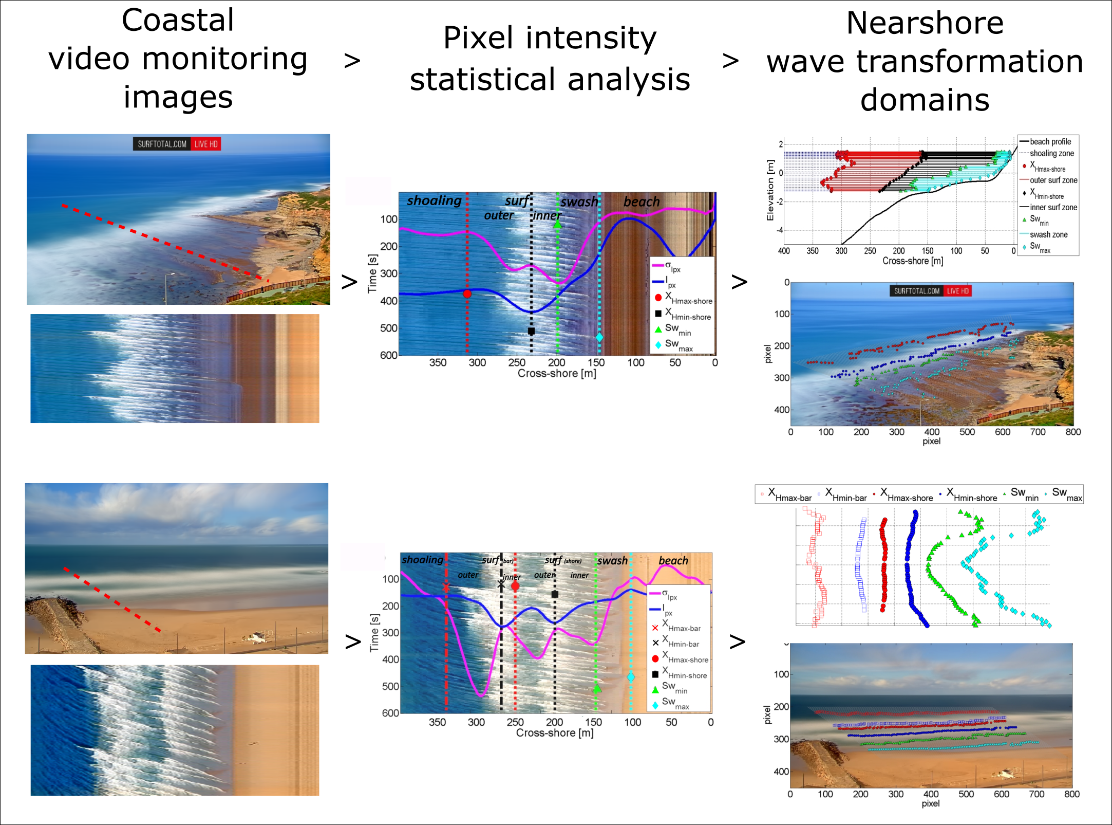
:Within the nearshore area, three wave transformation domains can be distinguished based on the wave properties: shoaling, surf, and swash zones. The identification of these distinct areas is relevant for understanding nearshore wave propagation properties and physical processes, as these zones can be related, for instance, to different types of sediment transport. This work presents a technique to automatically retrieve the nearshore wave transformation domains from images taken by coastal video monitoring stations. The technique exploits the pixel intensity variation of image acquisitions, and relates the pixel properties to the distinct wave characteristics. This allows the automated description of spatial and temporal extent of shoaling, surf, and swash zones. The methodology was proven to be robust, and capable of spotting the three distinct zones within the nearshore, both cross-shore and along-shore dimensions. The method can support a wide range of coastal studies, such as nearshore hydrodynamics and sediment transport. It can also allow a faster and improved application of existing video-based techniques for wave breaking height and depth-inversion, among others.
Keywords:
hydrodynamics; beach; coast; remote sensing; shoaling; surf zone; swash zone; wave runup; shoreline; bathymetry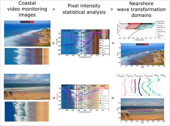
1. Introduction
The nearshore coastal region is defined as the area between the offshore limit and the shoreline [1,2]. The offshore limit indicates the location where the seabed starts affecting the wave, usually taken to be where the water depth is equal to half the deep-water wavelength, e.g., [1,2]. The shoreline is commonly defined as the edge between water and sand on the beach [3].
There is a continuous exchange of sediment between shoreline and offshore limit, driven by the incident wave climate and the alternations between storm and fair weather conditions [4,5]. At the same time, nearshore bottom configuration influences the effect of waves and the way in which coastal evolution occurs through the erosion, transport, and deposition of sediment material, either eroded by waves and currents or brought to the coast by rivers [4,5].
Within the nearshore area, based on the wave properties, three distinct zones can be distinguished: shoaling, surf, and swash zones. In the shoaling zone, waves coming from deep sea start to alter their shape in response to sea bed interaction. In general terms, wave height increases, wave speed decreases, and wave length decreases as wave orbits become asymmetrical, e.g., [6]. When the height of the wave becomes about the same size as the local water depth [7,8,9], the wave crest becomes too steep, it becomes unstable, curling forward and breaking. Hence, the surf zone is the area between the most seaward wave breaking point and the most landward broken wave [4,5]. The surf zone can be divided into two sub-regions [4,5]: outer breaking surf zone, where only some waves are breaking, and inner breaking surf zone, or saturated breaker zone, where all waves have collapsed, and travel as bore. Finally, the swash zone is the area in which the broken waves dissipate as swash on the beach foreshore slope [4,5]. This is also called intertidal area, because the swash beach area zone is above water during low tide and under water at high tide.
The shoaling, the surf and the swash zones are often also referred to as morphodynamic zones [10,11,12], since each zone is associated not only with a singular type of wave, but also to a particular sediment transport process. For example, Masselink [11] related the residence times of shoaling waves, breaking waves, and swash/backwash motions over a cross-shore profile, to sediment dynamics in the nearshore. In general, shoaling waves determine a relatively small onshore sediment transport, while large quantities of suspended sediment are transported offshore under breaking waves, e.g., [13,14]. Therefore, the identification of the different zones within the whole nearshore is beneficial for understanding coastal dynamic.
In most existing applications of the morphodynamic-zone approach to understand beach behavior [10,11,12], the boundary between the shoaling and surf zone was assumed to equal a specific wave height H to water depth h ratio. Nevertheless, several different ratios were used for H/h ratios (e.g., from H/h = 0.3 to H/h 0.8 in [10] and [11], respectively), since such a ratio is site-dependent and varies with wave conditions [15].
As many nearshore processes have a visible signature on the sea surface, remote sensing has emerged in this context as a valid alternative to provide nearshore measurements. Among numerous remote sensing methodologies and approaches (e.g., aerial photography, satellite imagery, wave radar, Light Detection And Ranging—LiDAR), shore-based coastal video monitoring has been proved as a cost-efficient and high-quality data collection tool to support coastal scientists and engineers over the last three decades [16,17].
Coastal video monitoring uses special images, namely Timex, Variance, and Timestack, produced through the acquired image sequences. These specific images have been considered “standard” since the advent of coastal video monitoring [16]. Time-Exposure images (Timex) are created by the mathematical average of RGB pixel intensity of the individual images collected over a period of sampling, usually chosen as 10 min, while Variance images are created by computing the standard deviation of the images within the period of video collection. A Timestack image is generated by sampling a single line of pixels from each image over the period of acquisition, and concatenating such an array of pixels according to the frame acquisition frequency. Timestack is therefore composed by pixel intensity time series over a given image sequence. For a detailed review of Timex, Variance, and Timestack coastal applications, please refer to [17] and references therein.
Exploiting video imagery properties, Price and Ruessink [14] improved the work of Masselink [11]. They quantified the hydrodynamic criteria to distinguish between the morphodynamic zones boundaries from a combination of field measurements and manual detection of breaking patterns on Timex images. However, the manually determined breakpoint positions on images were subjective and lacked the specific and rigorous criteria for the interpretation of image intensity variation given by breakers [14].
Overall, the existing morphodynamic-zone studies require the knowledge of nearshore bathymetry and/or the use of a wave propagation numerical model that simulates wave generation, shoaling, refraction, diffraction, and breaking, e.g., [14,18,19].
This work presents a methodology to identify the wave transformation domain boundaries from video imagery automatically. This is achieved by correlating Timestack image pixel intensity variation to wave features, and hence to wave transformation domains in the nearshore. As such pixel intensity variation can be observed also on Timex and Variance, the technique can be applied directly on these images, allowing the along-shore characterization of morphodynamic zones’ extent over time.
2. Concepts
2.1. Timestack Characteristics
Figure 1 illustrates the general characteristics and information that can be retrieved from Timestacks images. A Timestack image produced from surfcam image acquisition at Ribeira d’Ilhas beach (see Section 3) was chosen for the aim.
On Timestacks, pixel intensity characteristics can be related to water elevation due to the incident light reflection on the water surface, e.g., [20]. On Timestack, a timeseries of the wave trajectories can be seen over the chosen sampling period. When waves enter shallower waters, they shoal due to the change in water depth. The shadow created by the reduction of sunlight reflection on the water surface is visible on Timestacks as an abrupt drop in pixel intensity (Figure 1c), e.g., [21]. When the wave amplitude reaches a critical level [9,22,23], the wave breaks, creating turbulent whitewater spilling down its face. The typical white foam of breaking waves is visible on Timestacks as high-intensity white pixels [24,25,26,27]. Therefore, the incipient breaking point coincides with the change between dark and white pixels (Figure 1d) of each single wave feature visible on the image [24,25,26,27]. When broken waves reach the shore, they dissipate their energy in the form of wave swash on the emerged beach slope. Wave swash excursion patterns, or wave runup, are generally represented as cusplikes rhythmical in time [28,29,30], generated by the uprush and backwash movements on the foreshore slope (Figure 1f).
2.2. Timestack Pixel Intensity
In the nearshore, the simplest beach profile case typically decreases toward the shoreline. As real sea state is composed of irregular waves, the position of the breakpoint changes within the surf zone as a function of breaker height and water depth, e.g., [8]. For simplicity, it is further assumed that the highest waves break farther from the shoreline, whereas smaller waves break nearer the shore. Following this assumption, given the 10-min time interval used for Timestack production, the farthest breakpoint from the shore can be indicated as , since it represents the location where the highest wave broke. Likewise, the closest breakpoint to the shoreline coincides with the smallest breaking wave and can be indicated as the location where the smallest wave broke (). The minima and the maxima seaward discrete swash positions among all marked swash limits were defined as and , respectively.
Following the definitions of wave processes domains adopted and reported in Section 1, the boundary between shoaling and surf zone is identified by the first-occurring breaking point, coinciding therefore with . The shoreward breakpoint locates the boundary between outer and inner surf zones. Finally, the swash zone is comprised between the and , minimum and maximum swash excursions, respectively.
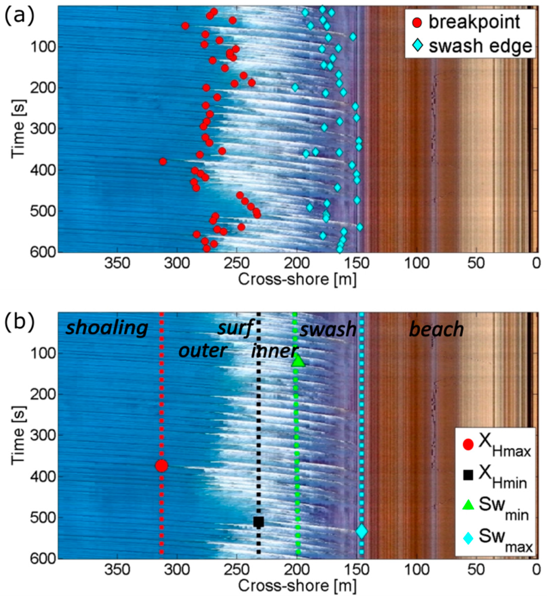
According to the conceptual descriptions of Timestack pixel characteristics in Section 2.1, breakpoints and swash locations can be visually identified and manually picked on Timestack (Figure 2a). Successively, single wave transformation processes can be manually recognized on Timestack identifying and as surf zone boundaries, with as the limit between outer and inner surf zone, and - as swash zone boundaries (Figure 2b). Hence, wave domains extent within the nearshore zone can be clearly determined from a visual analysis of Timestack.
3. Study Sites and Video Data
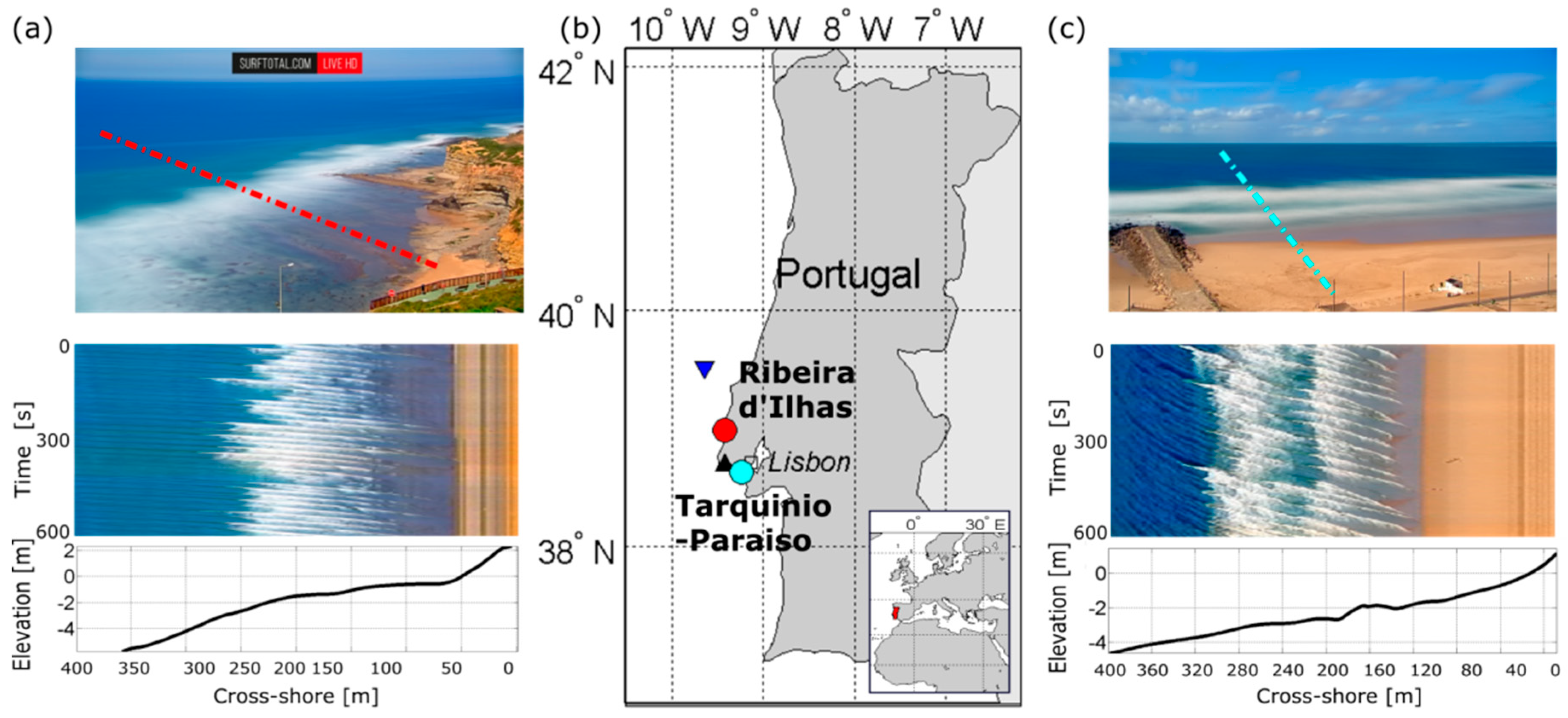
Two beaches are considered in the present study: Ribeira d’Ilhas beach and Tarquinio-Paraiso beach, on the North-Atlantic West Portuguese coast (Figure 3). The tidal regime is mesotidal, with average amplitude of the astronomical tide in the order of 2.10 m, reaching a maximum elevation of 4 m [31]. The dominant wave regime of the Portuguese western coast is characterized by waves coming from NW with average significant heights of 2 m and periods from 7 s to 15 s [32].
3.1. Ribeira d’Ilhas Beach
The Ribeira d’Ilhas beach (38°59′17.0″ N, 9°25′10.4″ W) develops on top of a rocky-shore platform located around 50 km north-west of Lisbon (Figure 1b). The beach extends for about 300 m cross-shore, with a NO-SE orientation, and it is limited southwards by 55 m high cliffs and in the north by a small headland. The collaboration with the company Surftotal allowed the use of the surfcam installed at Ribeira d’Ilhas [17]. The video station consists of a video camera mounted on a house roof at an elevation of about 80 m on the means sea level (MSL) and about 400 m from the Ribeira d’Ilhas beach. Around 18 hours of video bursts were retrieved during two days (28th and 29th of March 2017). Image frames were extracted at a frequency of 5 Hz. The whole dataset of 380000 frames (800 × 450 pixels resolution) was geo-rectified [33,34] and converted in a sequence of 52 10-min Timex Variance and Timestacks (Figure 1a) for the first day, 42 for the second day. The beach profile corresponding to Timestack transect was surveyed by LiDAR survey data.
Water level, which was retrieved from Cascais tide gauge (Figure 1), varied between a minimum of −0.94 m and a maximum of 1.8 m during both days, when the two flood tide phases were monitored. Offshore wave data were provided by the WaveScan buoy Monican (Figure 1b) deployed at 80 m depth (39.56°N, 9.21°W) by the Portuguese Hydrographic Institute Significant. Wave height (Hs) and peak period (Tp) were approximately constant on day 28 (1.7 m and around 11.5 s respectively) while on the 29th Hs increased from about 2 m to 3.5 m, whereas Tp decreased from 18 s to 16.5 s.
3.2. Tarquinio-Paraiso Beach
The Tarquinio-Paraiso beach (38°38′30.3″ N, 9°14′20.5″ W) is one of the sandy urban beaches included in Costa da Caparica, a coastal stretch located on the southern margin of the Tagus river inlet (Figure 3b). The beach extends for about 400 m along-shore, limited sideways by groins and landward by a seawall. Video data were acquired by a camera installed on the 8th floor of a hotel on 30th of October 2015. The dataset was composed of 61 videos, each one representing a 10-minute acquisition, from which 61 Timex Variance and Timestacks (Figure 3b) were generated. Unfortunately, the beach bathymetry survey for the video acquisition data was missing. The beach profile corresponding to Timestack transect was taken from a bathymetric survey from 2014, and should be considered as a rough estimation of water depth due to the high temporal variability of the sandy bottom morphology.
During the video monitored period, tidal level retrieved from Cascais tide gauge (Figure 3b) varied between a maximum value of 1 m and a minimum value of −1 m, with the first 5 hours of ebb tide phase and the last 5 hours of flood tide. Offhore wave conditions measured by Monican buoy were constant with Hs = 3.5 m and Tp = 12 s.
4. Methods
As seen from Timestack visual inspection (Figure 1 and Figure 2), the pixel brightness characterizes the representation of the different wave types. The manual procedure described in Section 2.2 is capable of identifying the wave transformation domains on Timestacks, however an automated technique would be beneficial for faster analysis and processing of video datasets.
This section describes the steps taken to relate pixel intensity variation to wave transformation domains, and automatically retrieve wave transformation boundaries.
4.1. Timestack Pixel Intensity Statistics
The variation of Timestack pixel intensity can be described by the average pixel intensity profile () and the standard deviation of the pixel intensity (), computed along the time-axis as follows:
and
where is the pixel intensity value and n the number of pixels.
The computation of is opportunistic because such pixel intensity values are the same as can be obtained by extracting the transect at the same location on Timex and Variance images, respectively [35].
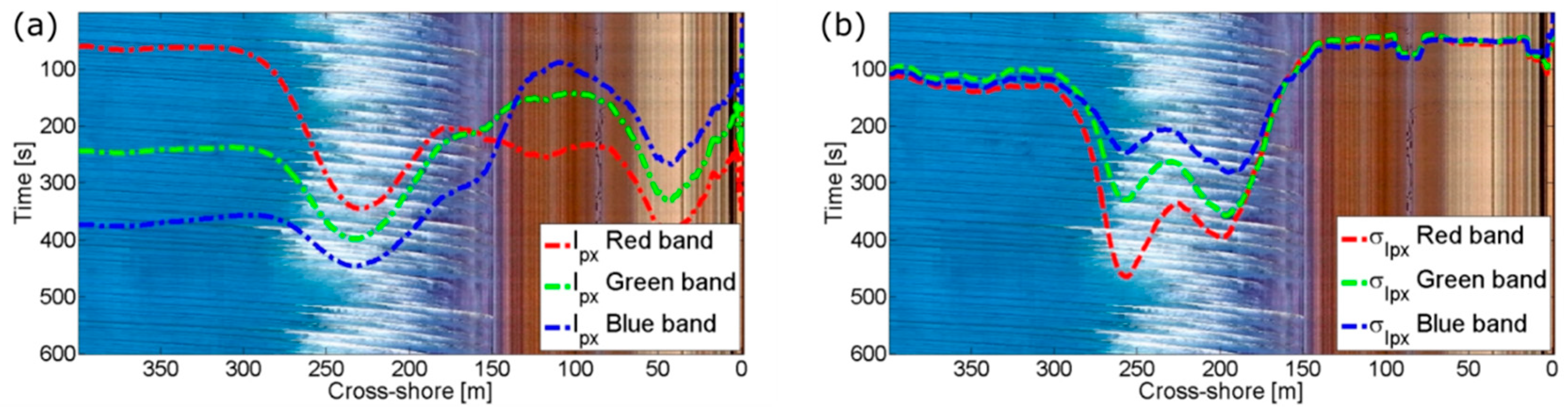
Figure 4 illustrates the shapes of the average pixel intensity (Figure 4a) and standard deviation (Figure 4b) over the profile. Timestack is a three band RGB image, therefore and profiles were computed for each colour band separately to be thorough. Signals were simply superimposed to the Timestack image to show their shape, as the absolute magnitude of intensity values are not in focus here. Note that on Timestack, and plots have an inverse y-axis due to Matlab convention for image axis.
profiles were similar over the nearshore zone, whilst their shapes diverged considerably over the swash zone. The profiles had similar shapes, differing only in intensity values. From hereinafter, the single Blue band was considered for both the and profiles, since both dark-blue shoaling and white-breaking waves are better represented by Blue colour band.
4.2. Timestack Pixel Intensity Statistics—Not Barred Beach
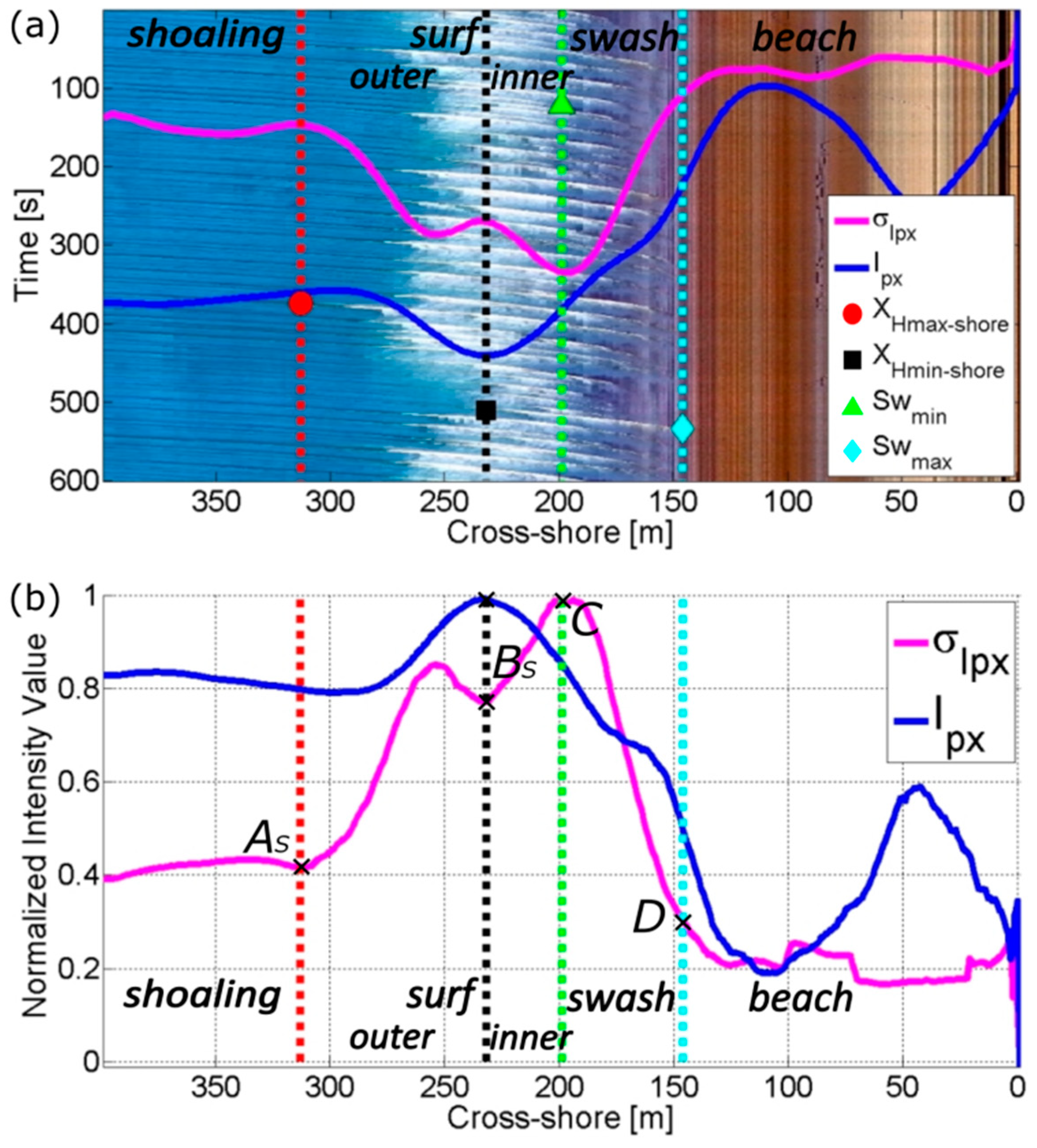
Figure 5a shows the single Blue band of and superimposed on the Timestack of Ribeira d’Ilhas, which was chosen among the 94 Timestacks composing the dataset. Besides, the unity-based Min–Max normalizations of and are shown in Figure 5b. Both pixel intensity statistics ( and ) were coupled to the visual breakpoint locations previously marked on Timestack (Section 3.2 and Figure 3), representing the transitions points between different wave domains, namely , , , and .
The average of pixel intensity was characterized by an almost constant value in the shoaling zone and by a Gaussian-like shape in the breaking zone [36,37], where the white foam of breaking waves increased the brightness value. In the analysed Timestack, the peak of the Gaussian-like shape coincided with the limit between the outer and inner surf zones, . Finally, dropped at the location of the dry beach and was not related to swash zone boundaries.
The was almost constant in the shoaling zone, where the pixel intensity variability did not change as a consequence of a regular shoaling waves patterns over time. The signal started to increase at the first incipient breaking wave, whose location delimitated the boundary between shoaling and the outer surf zone ( on Figure 5a, and point As in Figure 5b, where the subscript S stays for “shore”). In the outer surf zone, some waves are breaking and some are still shoaling towards the shore. Successively, reached a first local maximum, after which it decreased to a local minimum value (point BS) whose position coincided with the last incipient wave breaking point , and therefore delimited the boundary between the outer and inner surf zone (see also maximum of profile).
Yet, increased till reaching a second peak (point C), which identified the minimum wave swash position and the start of the area in which swash processes occurred. After such a position, drastically dropped till a minimum value (point D) which approximated and the boundary between wet sand and dry beach area.
Table 1 resumes the relationships that were found between wave domain transformations boundaries and the pixel intensity variations. Overall, was characterized by a bimodal distribution, under whose limits surf and swash zones were comprised (points AS-D). The valley between the two maxima of the distribution (point BS) coincided with the boundary between outer and inner surf zones, whereas the most shoreward maximum of the distribution located the edge between inner surf and swash zones (point C). Instead, was characterized by a single Gaussian-like shape whose main peak identified the boundary between inner and outer surf zone.
4.3. Timestack Pixel Intensity Statistics—Barred Beach
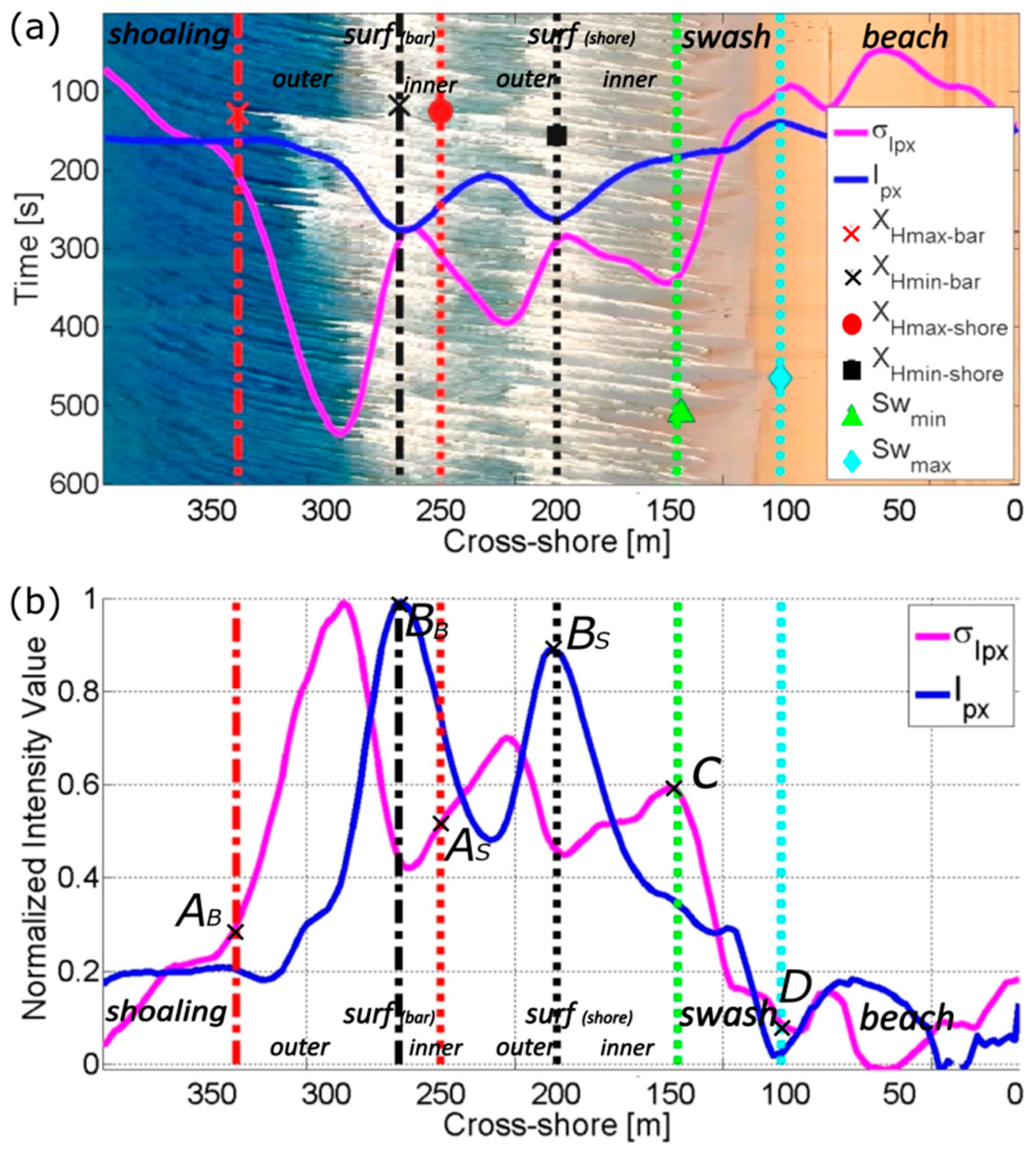
Figure 6 shows the single Blue band of and superimposed on the Timestack of Tarquinio-Paraiso, which was chosen among the 61 Timestacks composing the dataset. The nearshore bathymetry of the beach transect corresponding to Timestack transect was not available, however the presence of more than one preferential breaking point on the image clearly indicates the presence of barred beaches, e.g., [37,38,39].
Following the manual procedure presented in Section 3.1, the first seaward breaking point () and the last breaking point over the (theoretical) presence of the bar () were picked manually (Figure 6a). The same procedure was repeated marking , , and .
The average of pixel intensity (Figure 6a) showed two main peaks, as typically observed on barred beaches [20,37]. In the analysed Timestack, the peak of the Gaussian-like shape coincided with the limit between the outer and inner surf zones on bar, , while the second peak coincided with the limit between the outer and inner surf zones, as previously observed for the not-barred beach (Figure 5). Finally, dropped at the location of the dry beach and was not related to swash zone boundaries. The was almost constant in the shoaling zone. AS in the case of the not-barred beach (Figure 5), the signal started to increase at the first incipient breaking wave, whose location delimitated the boundary between shoaling and the outer surf bar zone ( on Figure 6a, and point AB, where the subscript B stays for “bar”, in Figure 6b). Successively, reached a first local maximum, after which it decreased to a local minimum value (point BB) whose position coincided with the last incipient wave breaking point , and therefore delimited the boundary between outer and inner surf bar zone (see also the first peak of profile). From here, increased showing the same configuration previously seen for the not-barred beach (Figure 5).
The valley between the two maxima of the distribution (point BS) coincided with the boundary between outer and inner surf zones, whereas the most shoreward maximum of the distribution located the edge between inner surf and swash zones (point D) which identified the minimum wave swash position and the start of the area in which swash processes occurred. After this position, drastically dropped until a minimum value (point D) which approximated the boundary between wet sand and dry beach area (). Table 2 resumes the relationships that were found between wave domain transformations boundaries and the pixel intensity variations.
4.4. Automated Algorithm
A dedicated algorithm was implemented to automatically recognize the particular points coinciding with the wave transformation boundaries on . The pixel intensity statistics profiles obtained from pixel analysis of Timestack, namely on , are the same as those that can be obtained by extracting the transect at the same location on Timex and Variance images, respectively [35]. The steps undertaken by the Matlab-based wave transformation domain detection algorithm are the following:
- Masking dry beach. The colour ratio Red:Green bands is computed from Timex profile. Following existing works [40], a value of Red:Green ratio of about 0.9 can be used to identify shoreline on coastal images. Here, a conservative value of 1.4 was used to filter out the emerged beach on profiles;
- Min–Max normalization of the Blue band . The pixel intensity statistical values of are transformed to the range 0–1.
- Smoothing data. are smoothed with a moving average window of 5% and 10% of the total Timestack space dimension, respectively. The window of is larger due to the fact that is generally more noise.
- Definition of numbers of breaking lines. The number of peaks on profile peaks are detected with the Matlab-built in function peakfinder in order to count the breaking lines (BB and/or BS). These point(s) represent also the boundary between outer and inner surf zones and , respectively.
- Identification of shoaling–surf zones boundary. The first breaking wave locations and/or (AB and/or AS) are recognized computing the first derivative of the profile, which returns the value of the slope of the signal. The locations AB and/or AS are found as the first derivative of exceeding the threshold value = 0.002 before BB and/or BS, respectively.
- Identification of surf–swash zone boundary. The location of (point C) is identified as the highest peak of after BS.
- Identification of swash zone landward limit. The location of (point D) is identified as the first local minima after D landward.
The algorithm is implemented in Matlab and is available from the author upon request.
5. Results
This section reports the performance of the automated algorithm for wave transformation boundaries detection, and further presents the potential applications of the presented technique for the analysis of the nearshore zone.
5.1. Automated Detection Performance
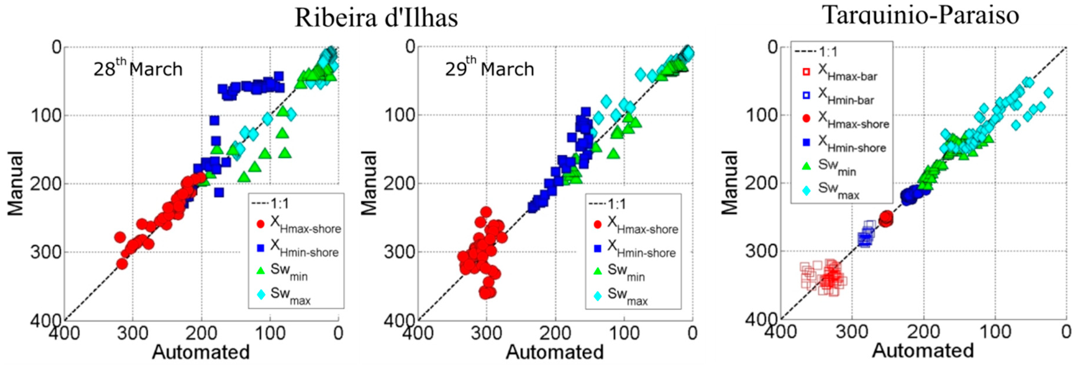
Figure 7 presents the relationships between manual procedure (Section 3.2) applied on Timestacks datasets and the specific points automatically detected on and . Pixel intensity statistics and were taken directly from Timex and Variance images, respectively, sampling the same transect used for producing Timestack images.
Overall the automatic detection performance was satisfactory for both the study sites, and mostly for all the considered specific points.
For Tarquinio-Paraiso, all the wave domain boundaries were clearly identified and matched the points detected on Timestacks. Some small discrepancies were observed on detection. These errors were due to the low quality of Variance images produced from the start of the video acquisition, which occurred during very low sun brightness at sunrise.
Lower accuracy resulted from processing the 94 images from Ribeira d’Ilhas, despite the fact that this beach was not-barred and (theoretically) represented the simplest case for wave transformation domains detection. In particular, the detection of and the locations did not perform properly for around 40% of the points in comparison with manual marking, especially on images from the 28th of March. Regarding the boundary between outer and inner surf zone (), the imprecision was likely due to the anomalous pixel intensity variation generated by the high spatial irregularity of wave breakpoints over the cross-shore profile. Similarly, the high swash dissipation characteristic of the low gradient slope of Ribeira d’Ilhas generated high noise and several peaks on during low tide, which caused errors in the automated detection of the boundary inner surf–swash zone (). The error observed for shoaling–surf zones boundaries () on the second day were mainly due to changes in sun brightness, since the last images were acquired during sunset. In this case, the algorithm did not correctly identify the breakpoints. Nevertheless, maximum inaccuracy was about 60 m over a 450 m cross-shore profile. The maximum swash excursion () recognition was satisfactory, despite the anomalies in pixel intensity generated by the dry rocky platform (e.g., Figure 4 and Figure 5). This proved the goodness of the masking dry beach procedure (step i in Section 4.4).
5.2. Wave Transfomation Domains
Figure 8 shows an example of the temporal variation of wave transformation domains automatically identified at Ribeira d’Ilhas over half a tidal cycle (increasing tide, tidal-range of 3 m) on day 29. The first seaward breakpoint occurred almost at the same position, around 300 m from the basepoint, while the boundary between the outer and the inner surf zone moved constantly shoreward as the sea elevation increased (Figure 8a). The outer surf zone length varied between 85 m to 150 m, augmenting its length with dependence on tide and Hs (Figure 8b). The inner surf zone extent started to increase at the tidal level of −0.5 m, when the swash zone reached its maximum extension (Figure 8b). After that, inner surf and swash zones had a contrary trend, with the inner surf enlarging and the swash zone diminishing its length. In fact, as the outer–inner surf boundary was shifting over a milder beach slope, broken waves were travelling as bore and finally swashing over the almost-planar rocky shore platform.
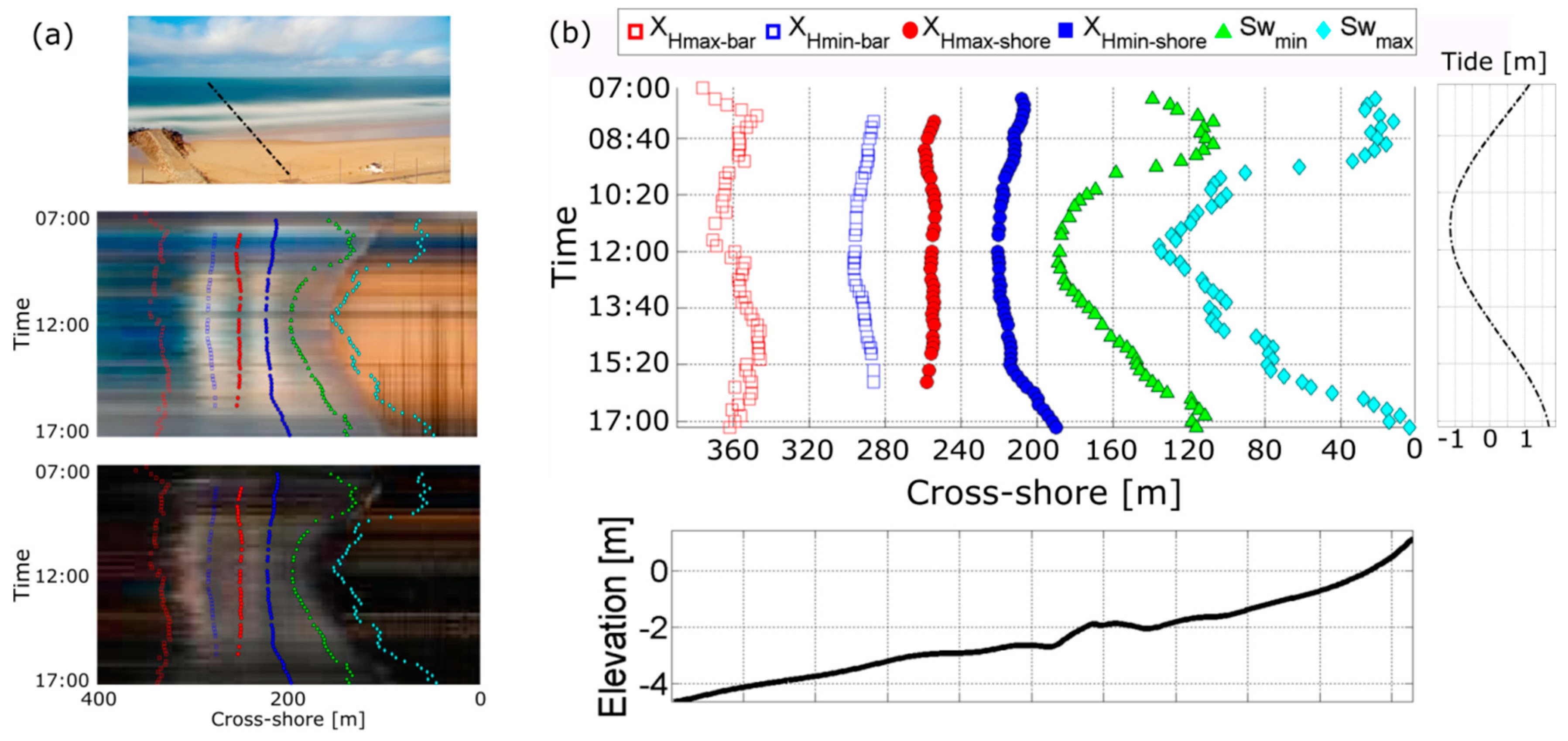
The analysis of wave transformation domains at Tarquinio-Paraiso (Figure 9) is shown with a second form of representation in respect to time and space. New images were generated sampling pixel timeseries over Timex (TimexStack) and Variance (VarStack) dataset (Figure 9a).
Over the 10 monitored hours, the position of and , as well as and did not vary significantly, since the offshore wave height was constant (Hs = 3.5 m). High dependence on tidal water level and beach slope was shown by the inner surf zone, suggesting predominance of surf bores during high tide, and by the swash zone, as here beach gradient was steeper. However, the lack of the beach profile survey corresponding to video data acquisition does not allow further analysis, besides the fact that morphodynamic zones variation analysis is beyond the purpose of this work.
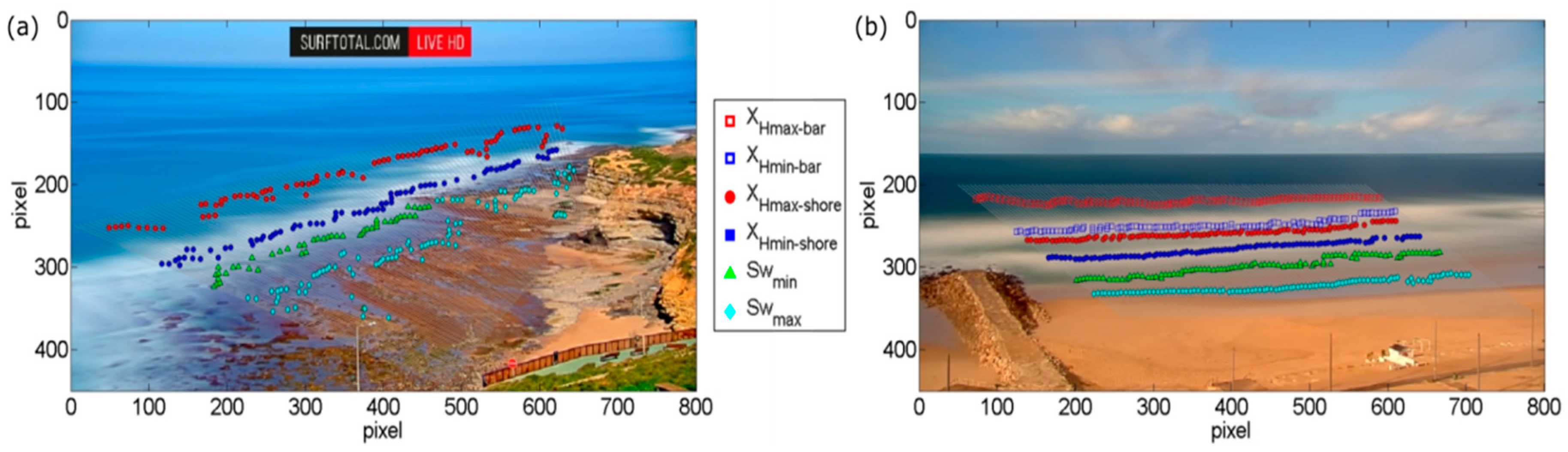
Since the presented methodology relies on the pixel intensity sampled on single profiles of Timex and Variance, the map of wave transformation domains boundaries can be obtained for the whole monitored area sampling a series of pixel transects on images, and applying the automated algorithm to each transect. Figure 10 shows an example of wave transformation domains boundaries over the whole monitored areas of both study sites, limited to a single Timex-Variance image analysis.
6. Discussion
The method provides a potential new tool to study the hydrodynamic changes and associated sediment transport within the nearshore. The approach offers an appropriate alternative to identify the wave transformation domain boundaries based on spatial variation of wave types, overcoming the subjectivity of visual determination on Timex used by Price and Ruessink [14], and the different hydrodynamic parameters proposed in previous works [10,11,12]. Besides, the application of the technique can help the improvement of nearshore wave dynamics insights, such as infragravity waves [41,42], surf and swash processes [43,44].
In addition to morphodynamic-zone studies, the technique can support the use of existing stand-alone automated procedures for coastal image analysis. Specific areas of the image can be previously extracted and/or masked to fasten, for instance, wave breaking height [25,45,46], rip currents [47,48,49,50], shoreline detection [35,51,52,53,54], wave runup measurements [30,35,55,56,57,58,59,60,61,62], and intertidal beach topography [28,29,36,61,63,64,65,66]. The use of the technique can also be coupled to the existing algorithm that focus on beach morphological features detection [67,68,69,70,71] for a fully description of coastal area from coastal imaging.
Of particular interest is the improvement that the presented methodology can give to video-based depth inversion technique [24,26,72,73,74,75,76]. For instance, as the methodology distinguishes between shoaling, breaking, and bore zones, its application may allow the use of different depth inversion formulas (linear and non-linear) based on wave type. Moreover, previous Timestack-based works for bathymetry estimation [26,73,77,78] have found that wave celerity at breaking points can be overestimated about 2.5 times, leading to an overestimation of local depth up to 2.5 times. Therefore, the masking of the outer surf zone on Timestacks may help in not considering breaking wave patterns for the cross-shore wave celerity computation.
The possibility of detecting wave transformation domain boundaries directly on Timex and Variance offers the advantage of extending such studies to the along-shore dimension, avoiding the computing-demanding generation of numerous Timestacks. The use of Variance is beneficial in respect to Timex, as these types of images are less sensitive to brightness. The automated detection algorithm can be improved to just consider the use of Variance for wave domains identification, as all the main boundaries can be detected on these images (Table 1 and Table 2). In addition, on RGB Variance the color band signals do not vary in trend (Figure 4), therefore the methodology can be applied, for instance, on gray Variance images. Nevertheless, . is generally noisier than Timex. For this reason, a higher level of smoothing was necessary for .than for (see Section 4.4).
The algorithm developed to identify the specific points on a signal was found to work fairly. However, it has been shown that in particular conditions, such as saturated surf zone and/or poor-quality images, the specific points can be roughly detected. These suggest that the likely limitations of the technique are related to the sea state conditions. For example, the clear identification of the boundaries between the different zones can be difficult if wave features (both shoaling and breaking) are not well visible. Swell conditions are ideal for the application, since shoaling and regular breaking wave patterns are well observable on images and thus detectable on .than for . Image quality is also important, weather conditions and sun reflection on sea surface being crucial for the correct application of the proposed methodology. For instance, pixel intensity variation of images acquired during foggy days, darkness, or rainy conditions might result in images being unusable. In addition, sun glitter and clouds might induce anomalous pixel intensity statistics, especially on profile. Taken into account that all these weather-related factors commonly occur in a natural environment, the technique robustness might be improved using a relatively large dataset to profit from time windows during favorable conditions.
Future work could investigate the relation between wave breaking fraction in the outer surf zone and pixel intensity statistics and , in order to improve the description of wave hydrodynamics in the nearshore from Timex and Variance images.
7. Conclusions
This paper presented a video-based methodology that allows the clear identification of shoaling, surf, and swash zones on coastal video images automatically. It was proved that the pixel intensity statistics of Timex and Variance images can be related to the specific wave transformation domain boundaries.
The performance of an automated algorithm developed for the detection of the specific wave transformation domain boundaries was validated with a manual procedure applied on Timestacks. Images acquired at two morphologically-different study sites were analysed for the successful validation of the technique, which allowed the detailed description of the spatial and temporal variation of wave transformation domains in the nearshore.
The applications of the methodology are numerous and cover both nearshore hydrodynamics and morphological studies. Besides, the automated classification of non-breaking and breaking zones can support and improve existing automated algorithms that exploit video imagery for estimating wave breaking height and for measuring wave celerity for depth-inversion techniques.
Funding
The author is supported by the project UAS4LITTER (PTDC/EAM-REM/30324/2017) funded by the Portuguese Foundation for Science and Technology (FCT). The publication was partially developed during the EARTHSYSTEM Doctorate Programme led by Instituto Dom Luiz at the University of Lisbon (SFRH/BD/52558/2014). The author also acknowledges the financial help of the FCT projects To-SEAlert (PTDC/EAM-OCE/31207/2017) and BSAFE4SEA (PTDC/ECI-EGC/31090/2017).
Acknowledgments
The author wishes to acknowledge Rui Taborda and Cristina Lira for their precious comments which improved the technique; Elena Sanchez-Garcia for the fundamental help in video imaging rectification process of both study sites; Diogo Mendes for the essential support in fieldwork at Ribeira d’Ilhas. Thanks go also to Ana Bastos and Andre Fortunato for their help in survey data collection at Ribeira d’Ilhas.
Conflicts of Interest
The author declares no conflict of interest.
References
- Svendsen, I.A. Introduction to Nearshore Hydrodynamics; University of Delaware: Newark, DE, USA, 2005; ISBN 978-981-256-142-8. [Google Scholar]
- Davies, J.L. Geographical Variation in Coastal Development. Geogr. J. 2006, 139, 350. [Google Scholar]
- Boak, E.H.; Turner, I.L. Shoreline Definition and Detection: A Review. J. Coast. Res. 2005, 214, 688–703. [Google Scholar] [CrossRef]
- Davidson-Arnott, R. Wave-Dominated Coasts. In Treatise on Estuarine and Coastal Science; Elsevier Science Publishing Co Inc.: San Diego, CA, USA, 2012; Volume 3, pp. 73–116. ISBN 9780080878850. [Google Scholar]
- Van Rijn, L.C. Principles of Sediment Transport in Rivers, Estuaries and Coastal Seas; Aqua Publications: Amsterdam, The Netherlands, 1993. [Google Scholar]
- Elgar, S.; Guza, R.T. Shoaling gravity waves: Comparisons between field observations, linear theory, and a nonlinear model. J. Fluid Mech. 1985, 158, 47–70. [Google Scholar] [CrossRef]
- Gaughan, M.K.; Komar, P.D. The theory of wave propagation in water of gradually varying depth and the prediction of breaker type and height. J. Geophys. Res. 1975, 80, 2991–2996. [Google Scholar] [CrossRef]
- Kamphuis, J.W. Incipient wave breaking. Coast. Eng. 1991, 15, 185–203. [Google Scholar] [CrossRef]
- McCowan, J. On the highest wave of permanent type. Philos. Mag. J. Sci. 1894, 5, 351–358. [Google Scholar] [CrossRef]
- Masselink, G.; Kroon, A.; Davidson-Arnott, R.G.D. Morphodynamics of intertidal bars in wave-dominated coastal settings—A review. Geomorphology 2006, 73, 33–49. [Google Scholar] [CrossRef]
- Masselink, G. Simulating the effects of tides on beach morphodynamics. J. Coast. Res. 1993, SI 15, 180–197. [Google Scholar]
- Kroon, A.; Masselink, G. Morphodynamics of intertidal bar morphology on a macrotidal beach under low-energy wave conditions, North Lincolnshire, England. Mar. Geol. 2002, 190, 591–608. [Google Scholar] [CrossRef]
- Beach, R.A.; Sternberg, R.W. Suspended sediment transport in the surf zone: Response to incident wave and longshore current interaction. Mar. Geol. 1992, 108, 275–294. [Google Scholar] [CrossRef]
- Price, T.D.; Ruessink, B.G. Morphodynamic zone variability on a microtidal barred beach. Mar. Geol. 2008, 251, 98–109. [Google Scholar] [CrossRef]
- Raubenheimer, B.; Guza, R.T.; Elgar, S. Wave transformation across the inner surf zone. J. Geophys. Res. C Ocean. 1996, 101, 25589–25597. [Google Scholar] [CrossRef]
- Holman, R.A.; Stanley, J. The history and technical capabilities of Argus. Coast. Eng. 2007, 54, 477–491. [Google Scholar] [CrossRef]
- Andriolo, U.; Sánchez-García, E.; Taborda, R. Operational Use of Surfcam Online Streaming Images for Coastal Morphodynamic Studies. Remote Sens. 2019, 11, 78. [Google Scholar] [CrossRef]
- Booij, N.; Holthuijsen, L.H.; Ris, R.C. The “Swan” Wave Model for Shallow Water. In Proceedings of the 25th International Conference on Coastal Engineering, Orlando, FL, USA, 2–6 September 1996. [Google Scholar]
- Zijlema, M.; Stelling, G.; Smit, P. SWASH: An operational public domain code for simulating wave fields and rapidly varied flows in coastal waters. Coast. Eng. 2011, 58, 992–1012. [Google Scholar] [CrossRef]
- Lippmann, T.C.; Holman, R.A. Quantification of sand bar morphology: A video technique based on wave dissipation. J. Geophys. Res. 1989, 94, 995–1011. [Google Scholar] [CrossRef]
- Catalán, P.; Haller, M.C. Nonlinear Phase Speeds and Depth Inversions. Coast. Dyn. 2005, 2006, 1–14. [Google Scholar]
- Salmon, J.E.; Holthuijsen, L.H.; Zijlema, M.; van Vledder, G.P.; Pietrzak, J.D. Scaling depth-induced wave-breaking in two-dimensional spectral wave models. Ocean Model. 2015, 87, 30–47. [Google Scholar] [CrossRef]
- Camenen, B.; Larson, M. Predictive Formulas for Breaker Depth Index and Breaker Type. J. Coast. Res. 2007, 234, 1028–1041. [Google Scholar] [CrossRef]
- Yoo, J.; Fritz, H.; Haas, K. Depth Inversion in the Surf Zone with inclusion of wave nonlinearity using video-derived celerity. J. Waterw. 2010, 137, 95–106. [Google Scholar] [CrossRef]
- Almar, R.; Cienfuegos, R.; Catalán, P.A.; Michallet, H.; Castelle, B.; Bonneton, P.; Marieu, V. A new breaking wave height direct estimator from video imagery. Coast. Eng. 2012, 61, 42–48. [Google Scholar] [CrossRef]
- Catálan, P.A.; Haller, M.C. Remote sensing of breaking wave phase speeds with application to non-linear depth inversions. Coast. Eng. 2008, 55, 93–111. [Google Scholar] [CrossRef]
- Flores, A.R.; Catalán, P.A.; Haller, M.C.M. Incorporating Remotely-Sensed Roller Properties Into Set-Up Estimations for Random Wave Conditions. Coast. Dyn. 2013, 2013, 615–626. [Google Scholar]
- Vousdoukas, M.I.; Ferreira, P.M.; Almeida, L.P.; Dodet, G.; Psaros, F.; Andriolo, U.; Taborda, R.; Silva, A.N.; Ruano, A.; Ferreira, Ó.M. Performance of intertidal topography video monitoring of a meso-tidal reflective beach in South Portugal. Ocean Dyn. 2011, 61, 1521–1540. [Google Scholar] [CrossRef]
- Andriolo, U.; Almeida, L.P.; Almar, R. Coupling terrestrial LiDAR and video imagery to perform 3D intertidal beach topography. Coast. Eng. 2018, 140, 232–239. [Google Scholar] [CrossRef]
- Stockdon, H.F.; Holman, R.A.; Howd, P.A.; Sallenger, A.H. Empirical parameterization of setup, swash, and runup. Coast. Eng. 2006, 53, 573–588. [Google Scholar] [CrossRef]
- Antunes, C.; Taborda, R. Sea Level at Cascais Tide Gauge: Data, Analysis and Results. J. Coast. Res. 2009, 1, 218–222. [Google Scholar]
- Dodet, G.; Bertin, X.; Taborda, R. Wave climate variability in the North-East Atlantic Ocean over the last six decades. Ocean Model. 2010, 31, 120–131. [Google Scholar] [CrossRef]
- Sánchez-García, E.; Balaguer-Beser, A.; Pardo-Pascual, J.E. C-Pro: A coastal projector monitoring system using terrestrial photogrammetry with a geometric horizon constraint. ISPRS J. Photogramm. Remote Sens. 2017, 128, 255–273. [Google Scholar] [CrossRef] [Green Version]
- Taborda, R.; Silva, A. COSMOS: A lightweight coastal video monitoring system. Comput. Geosci. 2012, 49, 248–255. [Google Scholar] [CrossRef]
- Simarro, G.; Bryan, K.R.; Guedes, R.M.C.; Sancho, A.; Guillen, J.; Coco, G. On the use of variance images for runup and shoreline detection. Coast. Eng. 2015, 99, 136–147. [Google Scholar] [CrossRef]
- Aarninkhof, S.G.J.; Turner, I.L.; Dronkers, T.D.T.; Caljouw, M.; Nipius, L. A video-based technique for mapping intertidal beach bathymetry. Coast. Eng. 2003, 49, 275–289. [Google Scholar] [CrossRef]
- Aarninkhof, S.G.J.; Ruessink, B.G. Video observations and model predictions of depth-induced wave dissipation. IEEE Trans. Geosci. Remote Sens. 2004, 42, 2612–2622. [Google Scholar] [CrossRef]
- Angnuureng, D.B.; Almar, R.; Senechal, N.; Castelle, B.; Addo, K.A.; Marieu, V.; Ranasinghe, R. Shoreline resilience to individual storms and storm clusters on a meso-macrotidal barred beach. Geomorphology 2017, 290, 265–276. [Google Scholar] [CrossRef]
- Armaroli, C.; Ciavola, P. Dynamics of a nearshore bar system in the northern Adriatic: A video-based morphological classification. Geomorphology 2011, 126, 201–216. [Google Scholar] [CrossRef]
- Almar, R.; Ranasinghe, R.; Sénéchal, N.; Bonneton, P.; Roelvink, D.; Bryan, K.R.; Marieu, V.; Parisot, J.P. Video-Based Detection of Shorelines at Complex Meso–Macro Tidal Beaches. J. Coast. Res. 2012, 28, 1040–1048. [Google Scholar]
- Mendes, D.; Pinto, J.P.; Pires-Silva, A.A.; Fortunato, A.B. Infragravity wave energy changes on a dissipative barred beach: A numerical study. Coast. Eng. 2018, 140, 136–146. [Google Scholar] [CrossRef]
- Moura, T.; Baldock, T.E. Remote sensing of the correlation between breakpoint oscillations and infragravity waves in the surf and swash zone. J. Geophys. Res. Ocean. 2017, 122, 3106–3122. [Google Scholar] [CrossRef]
- Almar, R.; Almeida, P.; Blenkinsopp, C.; Catalan, P. Surf-Swash Interactions on a Low-Tide Terraced Beach. J. Coast. Res. 2016, 75, 348–353. [Google Scholar] [CrossRef]
- Almar, R.; Nicolae Lerma, A.; Castelle, B.; Scott, T. On the influence of reflection over a rhythmic swash zone on surf zone dynamics. Ocean Dyn. 2018, 68, 899–909. [Google Scholar] [CrossRef]
- Shand, T.D.; Bailey, D.G.; Shand, R.D. Automated Detection of Breaking Wave Height Using an Optical Technique. J. Coast. Res. 2012, 28, 671–682. [Google Scholar]
- Gal, Y.; Browne, M.; Lane, C. Automatic estimation of nearshore wave height from video timestacks. In Proceedings of the Proceedings—2011 International Conference on Digital Image Computing: Techniques and Applications, Noosa, QLD, Australia, 6–8 December 2011; pp. 364–369. [Google Scholar]
- Turner, I.L.; Whyte, D.; Ruessink, B.G.; Ranasinghe, R. Observations of rip spacing, persistence and mobility at a long, straight coastline. Mar. Geol. 2007, 236, 209–221. [Google Scholar] [CrossRef]
- Pitman, S.; Gallop, S.L.; Haigh, I.D.; Masselink, G.; Ranasinghe, R. Wave breaking patterns control rip current flow regimes and surfzone retention. Mar. Geol. 2016, 382, 176–190. [Google Scholar] [CrossRef] [Green Version]
- Gallop, S.L.; Bryan, K.R.; Coco, G.; Stephens, S.A. Storm-driven changes in rip channel patterns on an embayed beach. Geomorphology 2011, 127, 179–188. [Google Scholar] [CrossRef]
- Gallop, S.L.; Bryan, K.R.; Pitman, S.J.; Ranasinghe, R.; Sandwell, D.R.; Harrison, S.R. Rip current circulation and surf zone retention on a double barred beach. Mar. Geol. 2018, 405, 12–22. [Google Scholar] [CrossRef]
- Harley, M.D.; Andriolo, U.; Armaroli, C.; Ciavola, P. Shoreline rotation and response to nourishment of a gravel embayed beach using a low-cost video monitoring technique: San Michele-Sassi Neri, Central Italy. J. Coast. Conserv. 2014, 18, 551–565. [Google Scholar] [CrossRef]
- Angnuureng, D.B.; Almar, R.; Appeaning Addo, K.; Castelle, B.; Senechal, N.; Laryea, S.W.; Wiafe, G. Video Oberservation of Waves and Shoreline Change on the Microtidal James Town Beach in Ghana. J. Coast. Res. 2016, 75, 1022–1026. [Google Scholar] [CrossRef]
- Huisman, C.E.; Bryan, K.R.; Coco, G.; Ruessink, B.G. The use of video imagery to analyse groundwater and shoreline dynamics on a dissipative beach. Cont. Shelf Res. 2011, 31, 1728–1738. [Google Scholar] [CrossRef] [Green Version]
- Valentini, N.; Saponieri, A.; Molfetta, M.G.; Damiani, L. New algorithms for shoreline monitoring from coastal video systems. Earth Sci. Inform. 2017, 10, 495–506. [Google Scholar] [CrossRef]
- Senechal, N.; Coco, G.; Bryan, K.R.; Holman, R.A. Wave runup during extreme storm conditions. J. Geophys. Res. Ocean. 2011, 116, C07032. [Google Scholar] [CrossRef]
- Atkinson, A.L.; Power, H.E.; Moura, T.; Hammond, T.; Callaghan, D.P.; Baldock, T.E. Assessment of runup predictions by empirical models on non-truncated beaches on the south-east Australian coast. Coast. Eng. 2017, 119, 15–31. [Google Scholar] [CrossRef] [Green Version]
- Blenkinsopp, C.E.; Matias, A.; Howe, D.; Castelle, B.; Marieu, V.; Turner, I.L. Wave runup and overwash on a prototype-scale sand barrier. Coast. Eng. 2016, 113, 88–103. [Google Scholar] [CrossRef]
- Almar, R.; Blenkinsopp, C.; Almeida, L.P.; Catalán, P.A.; Bergsma, E.; Cienfuegos, R.; Viet, N.T. A new remote predictor of wave reflection based on runup asymmetry. Estuar. Coast. Shelf Sci. 2019, 217, 1–8. [Google Scholar] [CrossRef]
- Vousdoukas, M.I. Observations of wave run-up and groundwater seepage line motions on a reflective-to-intermediate, meso-tidal beach. Mar. Geol. 2014, 350, 52–70. [Google Scholar] [CrossRef]
- Guedes, R.M.C.; Bryan, K.R.; Coco, G.; Holman, R.A. The effects of tides on swash statistics on an intermediate beach. J. Geophys. Res. Ocean. 2011, 116, 1–13. [Google Scholar] [CrossRef]
- Vousdoukas, M.I.; Wziatek, D.; Almeida, L.P. Coastal vulnerability assessment based on video wave run-up observations at a mesotidal, steep-sloped beach. Ocean Dyn. 2012, 62, 123–137. [Google Scholar] [CrossRef]
- Almar, R.; Blenkinsopp, C.; Almeida, L.P.; Cienfuegos, R.; Catalán, P.A. Wave runup video motion detection using the Radon Transform. Coast. Eng. 2017, 130, 46–51. [Google Scholar] [CrossRef]
- Uunk, L.; Wijnberg, K.M.; Morelissen, R. Automated mapping of the intertidal beach bathymetry from video images. Coast. Eng. 2010, 57, 461–469. [Google Scholar] [CrossRef]
- Osorio, A.F.; Medina, R.; Gonzalez, M. An algorithm for the measurement of shoreline and intertidal beach profiles using video imagery: PSDM. Comput. Geosci. 2012, 46, 196–207. [Google Scholar] [CrossRef]
- Sobral, F.; Pereira, P.; Cavalcanti, P.; Guedes, R.; Calliari, L. Intertidal Bathymetry Estimation Using Video Images on a Dissipative Beach. J. Coast. Res. 2013, 165, 1439–1444. [Google Scholar] [CrossRef]
- Smit, M.W.J.; Aarninkhof, S.G.J.; Wijnberg, K.M.; González, M.; Kingston, K.S.; Southgate, H.N.; Ruessink, B.G.; Holman, R.A.; Siegle, E.; Davidson, M.; et al. The role of video imagery in predicting daily to monthly coastal evolution. Coast. Eng. 2007, 54, 539–553. [Google Scholar] [CrossRef]
- Hoonhout, B.M.; Radermacher, M.; Baart, F.; van der Maaten, L.J.P. An automated method for semantic classification of regions in coastal images. Coast. Eng. 2015, 105, 1–12. [Google Scholar] [CrossRef] [Green Version]
- Hoonhout, B.; Baart, F.; van Thiel de Vries, J. Intertidal beach classification in infrared images. J. Coast. Res. 2015, 70, 657–663. [Google Scholar] [CrossRef]
- Quartel, S.; Addink, E.A.; Ruessink, B.G. Object-oriented extraction of beach morphology from video images. Int. J. Appl. Earth Obs. Geoinf. 2006, 8, 256–269. [Google Scholar] [CrossRef]
- Rainey, K. Characterization of Sun Glitter Statistics in Ocean Video a NISE Funded Basic Research Project; Space and Naval Warfare Systems Center Pacific: San Diego, CA, USA, 2013. [Google Scholar]
- Revollo, N.V.; Delrieux, C.A.; Perillo, G.M.E. Automatic methodology for mapping of coastal zones in video sequences. Mar. Geol. 2016, 381, 87–101. [Google Scholar] [CrossRef]
- Holman, R.; Plant, N.; Holland, T. CBathy: A robust algorithm for estimating nearshore bathymetry. J. Geophys. Res. Ocean. 2013, 118, 2595–2609. [Google Scholar] [CrossRef]
- Almar, R.; Cienfuegos, R.; Catalán, P.; Birrien, F.; Castelle, B.; Michallet, H. Nearshore bathymetric inversion from video using a fully non-linear Boussinesq wave model. J. Coast. Res. 2011, 64, 3–7. [Google Scholar]
- Bergsma, E.W.J. Application of an Improved Video-Based Depth Inversion Technique to a Macrotidal Sandy Beach. Ph.D. Thesis, University of Plymouth, Plymouth, UK, 2017. [Google Scholar]
- Stockdon, H.F.; Holman, R.A. Estimation of wave phase speed and nearshore bathymetry from video imagery. J. Geophys. Res. Ocean. 2000, 105, 22015–22033. [Google Scholar] [CrossRef]
- Liu, H.; Arii, M.; Sato, S.; Tajima, Y. Long-Term Nearshore Bathymetry Evolution from Video Imagery: A Case Study in the Miyazaki Coast. Coast. Eng. Proc. 2012, 1, 60. [Google Scholar] [CrossRef]
- Tissier, M.; Almar, R.; Postacchini, M.; Castelle, B.; Bonneton, N.; Bretel, P. Field measurements of wave celerity in the surf zone, analysis of nonlinear and very low frequency processes. Eur. J. Mech. B/Fluids 2010, 1, 6–8. [Google Scholar]
- Postacchini, M.; Brocchini, M. A wave-by-wave analysis for the evaluation of the breaking-wave celerity. Appl. Ocean Res. 2014, 46, 15–27. [Google Scholar] [CrossRef]
Figure 1.
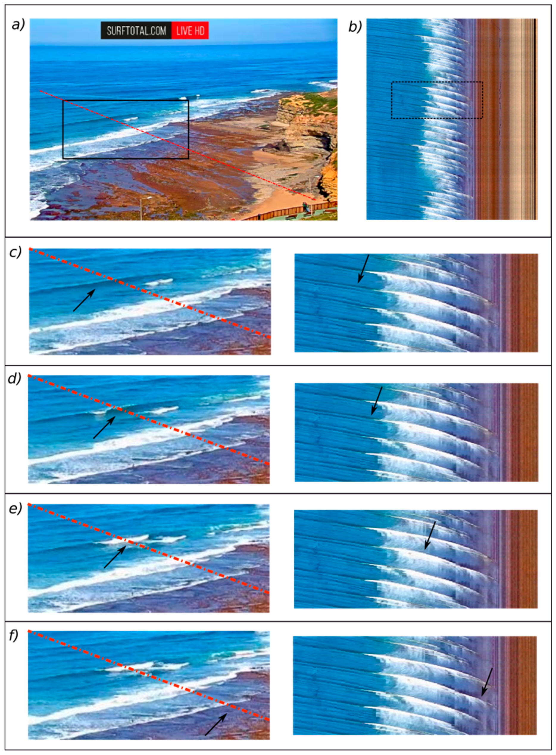
Waves characteristics on Timestacks. Sample taken from Ribeira d’Ilhas dataset. (a) Original image and transect (dashed red line) to generate the (b) 10-min Timestack. Black boxes indicate the image area reproduced in detail below. (c) Shoaling non-breaking waves troughs are represented as darker straight features on oblique (left) and Timestack image (right); (d) breakpoints coincide with the change in pixel intensity, from dark pixel (shoaling) to white pixel (breaking foam); (e) broken waves are represented by white pixel stripes on Timestakcs, whereas light white pixels represent ocean foam; (f) wave swash movements are identified by the rhythmic cusplikes in the swash zone.
Figure 1.
Waves characteristics on Timestacks. Sample taken from Ribeira d’Ilhas dataset. (a) Original image and transect (dashed red line) to generate the (b) 10-min Timestack. Black boxes indicate the image area reproduced in detail below. (c) Shoaling non-breaking waves troughs are represented as darker straight features on oblique (left) and Timestack image (right); (d) breakpoints coincide with the change in pixel intensity, from dark pixel (shoaling) to white pixel (breaking foam); (e) broken waves are represented by white pixel stripes on Timestakcs, whereas light white pixels represent ocean foam; (f) wave swash movements are identified by the rhythmic cusplikes in the swash zone.

Figure 2.
Visual and manual analysis of Timestack. (a) Single breakpoints (red circles) and swash edges (cyan diamonds) marked on Timestack; (b) wave transformation domains identified by the points marked on Timestack. Dashed colored lines identify the boundaries between wave domains.
Figure 2.
Visual and manual analysis of Timestack. (a) Single breakpoints (red circles) and swash edges (cyan diamonds) marked on Timestack; (b) wave transformation domains identified by the points marked on Timestack. Dashed colored lines identify the boundaries between wave domains.

Figure 3.
Study sites locations. (a) Timex image (upper), Timestack image (middle), and related beach profile (lower) at Ribeira d’Ilhas; (b) locations of the study sites. Blue and black triangles show offshore buoy and tide gauge positions, respectively; (c) Timex image (upper), Timestack image (middle), and related beach profile (lower) at Tarquinio-Paraiso beach. Note that the beach profile was not surveyed during video data acquisition and it is shown for a rough reference of bottom elevation.

Figure 4.
Timestack pixel intensity statistics, example with Timestack produced from Ribeira d’Ilhas images. (a) Averaged pixel intensity for Red (red line), Blue (blue line), and Green (green line) band of the Timestack; (b) standard deviation of pixel intensity for Red (red line), Blue (blue line), and Green (green line) band of Timestack. Note that and are superimposed to Timestack for description purposes and have an inverted y-axis unit.

Figure 5.
Timestack pixel intensity statistics combined with wave transformation domains at Ribeira d’Ilhas. (a) Wave transformation domains superimposed on Timestack combined with and . Dashed colored lines identify the boundaries between wave domains. (b) Min–Max (blue line) and (magenta) plotted together with wave transformation regions boundaries. The specific points on the signal coinciding with wave domain boundaries are indicated with related name and by black crosses (Table 1). Dashed colored lines identify the boundaries between wave domains.

Figure 6.
Timestack pixel intensity statistics combined with wave transformation domains at Tarquinio-Paraiso. (a) Wave transformation domains superimposed on Timestack combined with and . Dashed colored lines identify the boundaries between wave domains. (b) Min–Max (blue line) and (magenta line) plotted together with wave transformation regions boundaries. The specific points on signal which coincide with wave domain boundaries are indicated with related name and by black crosses (see also Table 2). Dashed colored lines identify the boundaries between wave domains.

Figure 7.
Automated detection performance against manual procedure. x and y axes show distances in m from the landward edge of the profile considered for Timestack production (see also Figure 4 and Figure 5).

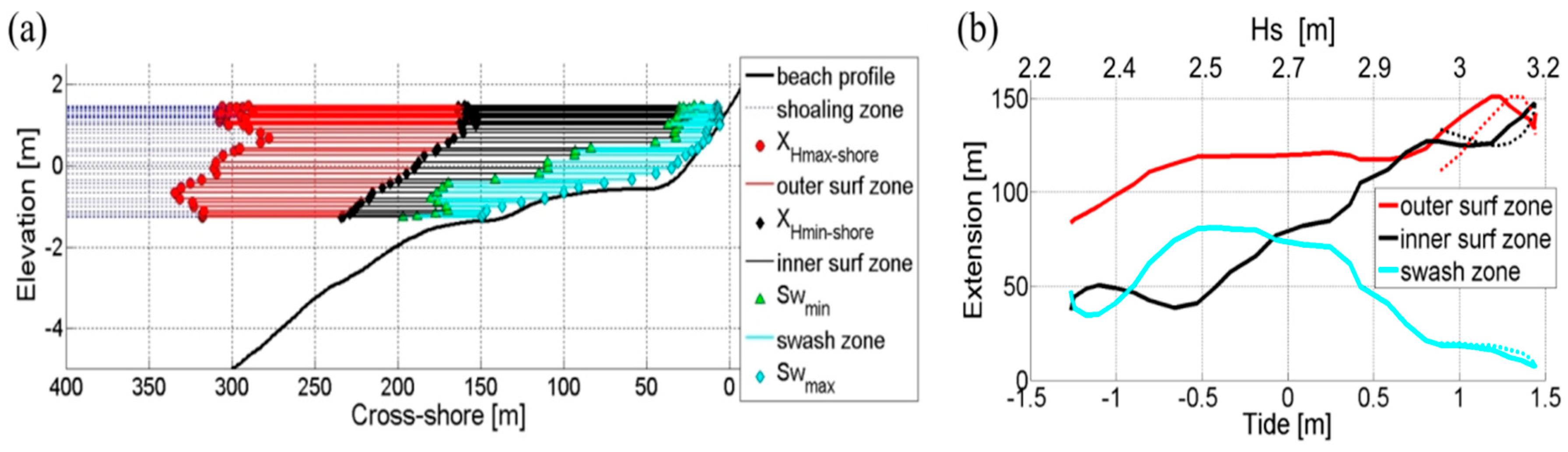
Figure 8.
Wave transformation domains spatial variation at Ribeira d’Ilhas on 29th of March. (a) Plot of the wave transformations domains extent over the beach profile, at the time-correlated tidal level. (b) Extension of inner, outer surf and swash zone in respect to wave significant height and tidal elevation. Dashed lines indicate ebb tide phase.

Figure 9.
Spatial and temporal variation of wave transformation domains at Tarquinio-Paraiso. (a) Wave transformations domains boundaries plotted on TimexStack (middle) and on VarStack (lower) images generated sampling the pixel transect (upper) over Timex and Variance dataset; (b) wave transformations domains boundaries plotted over space and time in relation to water level and beach profile. Note that beach profile does not correspond to survey during video data acquisition and it is shown for a rough reference of bottom elevation.

Figure 10.
Along-shore identification of wave transformation domain boundaries. (a) Example of spatial distribution of morphodynamic zone boundaries plotted on Timex image at Ribeira d’Ilhas; (b) example spatial distribution of morphodynamic zone boundaries plotted on Timex image at Tarquinio-Paraiso. Legend is common to both images.


Table 1.
Relation between wave transformation domain boundaries, breakpoints marked on Timestacks (see Figure 5a) and specific points identified on and plot (see Figure 5b).
| Wave Domain Boundary | Breakpoints | ||
|---|---|---|---|
| shoaling- surf zone | - | ||
| outer-inner surf zone | Bs | Bs | |
| surf – swash zone | Swmin | - | |
| swash zone-dry beach | Swmax | - |
Table 2.
Relation between wave transformation domain boundaries, breakpoints marked on Timestacks (see Figure 6a) and specific points identified on and (Figure 6b).
| Wave Domain Boundary | Breakpoints | ||
|---|---|---|---|
| shoaling- surf zone | - | B | |
| outer-inner surf zone | BB | BB | |
| shoaling- surf zone | S | S | |
| outer-inner surf zone | BS | BS | |
| surf – swash zone | Swmin | - | |
| swash zone-dry beach | Swmax | - |
© 2019 by the author. Licensee MDPI, Basel, Switzerland. This article is an open access article distributed under the terms and conditions of the Creative Commons Attribution (CC BY) license (http://creativecommons.org/licenses/by/4.0/).
Share and Cite
MDPI and ACS Style
Andriolo, U. Nearshore Wave Transformation Domains from Video Imagery. J. Mar. Sci. Eng. 2019, 7, 186. https://doi.org/10.3390/jmse7060186
AMA Style
Andriolo U. Nearshore Wave Transformation Domains from Video Imagery. Journal of Marine Science and Engineering. 2019; 7(6):186. https://doi.org/10.3390/jmse7060186
Chicago/Turabian StyleAndriolo, Umberto. 2019. "Nearshore Wave Transformation Domains from Video Imagery" Journal of Marine Science and Engineering 7, no. 6: 186. https://doi.org/10.3390/jmse7060186
Note that from the first issue of 2016, this journal uses article numbers instead of page numbers. See further details here.