All articles published by MDPI are made immediately available worldwide under an open access license. No special
permission is required to reuse all or part of the article published by MDPI, including figures and tables. For
articles published under an open access Creative Common CC BY license, any part of the article may be reused without
permission provided that the original article is clearly cited. For more information, please refer to
https://www.mdpi.com/openaccess.
Feature papers represent the most advanced research with significant potential for high impact in the field. A Feature
Paper should be a substantial original Article that involves several techniques or approaches, provides an outlook for
future research directions and describes possible research applications.
Feature papers are submitted upon individual invitation or recommendation by the scientific editors and must receive
positive feedback from the reviewers.
Editor’s Choice articles are based on recommendations by the scientific editors of MDPI journals from around the world.
Editors select a small number of articles recently published in the journal that they believe will be particularly
interesting to readers, or important in the respective research area. The aim is to provide a snapshot of some of the
most exciting work published in the various research areas of the journal.
The General Curvilinear Coastal Ocean Model (GCCOM) is a 3D curvilinear, structured-mesh, non-hydrostatic, large-eddy simulation model that is capable of running oceanic simulations. GCCOM is an inherently computationally expensive model: it uses an elliptic solver for the dynamic pressure; meter-scale simulations requiring memory footprints on the order of cells and terabytes of output data. As a solution for parallel optimization, the Fortran-interfaced Portable–Extensible Toolkit for Scientific Computation (PETSc) library was chosen as a framework to help reduce the complexity of managing the 3D geometry, to improve parallel algorithm design, and to provide a parallelized linear system solver and preconditioner. GCCOM discretizations are based on an Arakawa-C staggered grid, and PETSc DMDA (Data Management for Distributed Arrays) objects were used to provide communication and domain ownership management of the resultant multi-dimensional arrays, while the fully curvilinear Laplacian system for pressure is solved by the PETSc linear solver routines. In this paper, the framework design and architecture are described in detail, and results are presented that demonstrate the multiscale capabilities of the model and the parallel framework to 240 cores over domains of order total cells per variable, and the correctness and performance of the multiphysics aspects of the model for a baseline experiment stratified seamount.
As computational modeling and its resources becomes ubiquitous, numerical solutions to complex equations can be solved with increasing resolution and accuracy. At the same time, as more variables and processes are taken into account, and spatial and temporal resolutions are increased to model real field-scale events, models become more complex yet resource efficiency remains an important requirement. Multiscale and multiphysics modeling encompasses these factors and relies on High-Performance Computing (HPC) resources and services to solve problems effectively [1]. The models used for atmospheric and ocean studies are examples of such applications.
In atmospheric and ocean studies, one of the major challenges is the simulation of coastal ocean dynamics due to the vast range of length and time scales required: tidal processes and oceanic currents happen in fractions of days; wavelengths are scale lengths of kilometers; mixing and turbulence events need to be resolved at the meter or submeter scale; and time resolution is in terms of years to minutes or seconds. Consequently, field scale simulations need to cover both sides of the time/space spectrum while preserving accuracy, forcing the use of highly detailed grids of considerable size. The General Curvilinear Coastal Ocean Model (GCCOM) is a 3D, curvilinear, large-eddy simulation model designed specifically for high-resolution (meter scale) simulations of coastal regions, capable of capturing nonhydrostatic flow dynamics [2].
Another major challenge is the need to solve for nonhydrostatic pressures. Ocean and climate models are generally hydrostatic, limiting the physics they are able to capture, and large scale, so that they are computationally efficient enough to make forecasts in reasonable run-times. Historically, these models have opted to solve the more computationally efficient, but less accurate, hydrostatic version of the Navier–Stokes equations because simulating nonhydrostatic processes using the Boussinesq approximation is computationally intensive, as these models require solving an elliptic problem [3,4,5]. However, advances in HPC systems and algorithms have enabled the use of nonhydrostatic solvers in ocean models including GCCOM [6], MITgcm [7], SUNTANS [8], FVCOM [9], SOMAR [10], and KLOCAW [11].
A differentiating feature of these models is the method used to solve the nonhydrostatic pressure: the pressure can be either solved in the physical grid after taking the divergence of the momentum equation (Boussinesq), or reconstructed from the equation of state when density is chosen as the main scalar argument. In GCCOM, the pressure is solved on a fully 3D (not 2D plus sigma coordinates) computational grid (a normalized representation of the physical grid) that is created after applying a unique, general 3D curvilinear transformation to the Laplacian problem [2]. All computations are performed on the computational grid, which increases the accuracy of the results. The curvilinear coordinates formulation enforces the computational grid to be unitary and orthogonal, thus simplifying the boundary treatment and ensuring minimal energy loss by transforming any boundary geometry to an unitary cube, which in practice reduces the application of boundaries to a plane (or edge) of this cube. In contrast, the typical approach of approximating the grid cell to the problem geometry loses energy in the boundary proportional to the grid resolution. A detailed comparison of the GCCOM model with other non hydrostatic ocean models functionalities can be found in [12].
One other defining characteristic of some of these nonhydrostatic models is the HPC framework used: many use the Message Passing Interfae (MPI) framework (in some cases enhanced by using OpenMP, or accelerated using GPU resources), parallel file IO, and have large teams developing advanced multiphysics modules. Typically, these models are often nested within large, global, weather prediction models such as those used in disaster response situations, which is a long-term goal of this project. GCCOM is a modern model: written in Fortran 95; modular; employing NetCDF to manage the data. The first parallel version of an earlier GCCOM model (UCOAM) used a customized MPI-based parallel framework that scaled to a few hundred cores [13]. The UCOAM model has also been used for nesting inside the California ROMS global ocean model [14,15]. Having demonstrated the multiscale and multiphysics capabilities of GCCOM [12], the next phase of development requires a more advanced HPC framework in order to speed up development and testing and allow us to work with more realistic domains and algorithms. These factors motivated the decision to migrate the model to a more advanced HPC framework.
One additional factor in our project is the size of the team, and the level of effort needed to produce and support this type of model. Often the larger model projects are optimized for specific hardware that may not be portable. These models often require large development teams. One of the goals of the GCCOM project is to deliver a portable model that can run in a heterogeneous computing environment and proves useful to smaller research teams, but would someday scale to run inside of larger models. As the GCCOM model evolved, the PETSc (Portable-Extensible Toolkit for Scientific Computing) model was chosen to improve the scaling and efficiency of the model and to improve access to advanced mathematical libraries and tools [16,17,18]. The results presented in the paper justify the time and effort required to accomplish these objectives.
In this paper, the outcome of this approach is presented. The background of the model, motivation for parallelization, the parallel approach, and the choices for the underlying software stack are described in Section 2.1, Section 2.2, and Section 2.4. The methodology and specifics of the test case used to validate the parallel framework are described in Section 2.5 and the validated results showing that the parallelized model produces correct results are presented in Section 3.1. The parallel performance is presented in Section 3.2 with results showing that the prototype model scales with the PETSc framework and to the maximum size of the HPC system used for these tests. Section 3.3 contains results demonstrating the multiscale and multiphysics capabilities of the model. Conclusions and future work are discussed in Section 4.
2. Materials and Methods
2.1. The General Curvilinear Coastal Ocean Model (GCCOM)
The General Curvilinear Coastal Ocean Model (GCCOM) is a coastal ocean model that solves the three-dimensional Navier–Stokes equation with the Boussinesq approximation, a Large Eddy Simulation (LES) formulation is implemented with a subgrid-scale model, capable of handling strongly stratified environments [12]. GCCOM features include: an embedded fully 3D curvilinear transformation, which makes it uniquely equipped to handle non-convex features in every direction including along the vertical axis [2]; a full 3D curvilinear Laplacian operator that solve a 3D nonhydrostatic pressure equation that accurately reproduces features resulting from the interaction of currents and steep bathymetries; and ability to calculate solutions from the sub-meter to the kilometer ranges in one simulation. With these key features, GCCOM has been used to simulate coastal ocean processes with multiscale simulations ranging from oceanic currents and internal waves [15] to turbulence mixing and bores formation, all in a single scenario [19], as well as the use of data assimilation capabilities [20], including thermodynamics and turbulence mixing on high-resolution grids, up to meter and sub-meter scales. Additionally, a key goal of the GCCOM model is to study turbulent mixing and internal waves in the coastal region, as a way to bridge the work of regional models (e.g., ROMS [21] or POP [22]), and global models (e.g., MPAS [23], HYCOM [24]), all the way to the sea–land interface.
GCCOM was recently validated for stratified oceanographic processes in [12] and has been coupled with ROMS [15] using nested grids to obtain greater resolution in a region of interest, using approaches that are similar to the work of other coupled ocean model systems. In [25], an overset grid method is used to couple a hydrostatic, large scale, coastal ocean flow model (FVCOM or unstructured grid finite volume coastal ocean model) with a non-hydrostatic model tailored for high-fidelity, unsteady, small scale flows (SIFOM or solver for incompressible flow on overset meshes). This method presents a way to offset the computational cost of a single, comprehensive model capable of dealing with multiple types of physics. GCCOM is similar to SIFOM in the curvilinear transformation and multiphysics capabilities, but they differ in the basic grid layout (staggered vs. non-staggered grids) and in the numerical methods each one applies to solve the Navier–Stokes equations. In addition, GCCOM has been taking strides in its development so it does not need to couple with a large-scale model to capture multiscale processes. Instead, GCCOM includes the entire domain in the curvilinear, nonhydrostatic, multiphysics capable region, where we handle thermodynamics, hydrostatic and nonhydrostatic pressure and equation of state density distributions at the same time. In this sense, GCCOM is a model capable of supporting both multiphysics and multiscale calculations at high computational costs. Recently, the PETSc-based GCCOM model has been coupled with SWASH [26] to simulate surface waves and overcome the limitations of the rigid lid [27]. SWASH is a numerical tool used to simulate free-surface, rotational flow and transport phenomena in coastal waters, we used the hydrostatic component to capture and validate surface wave heights in a seamount testcase.
GCCOM development began with [28] introducing the 3D curvilinear coordinates transformation, along with practical applications including the Alarcon Seamount and Lake Valencia waters [29,30]. Later, the model was revised by [2] to add thermodynamic processes, the UNESCO Equation of State, and use of a simple Successive Over–Relaxation (SOR) algorithm to solve the non-hydrostatic pressure [31] on an Arakawa-C grid [32], and an upgrade of the model to Fortran 95. In order to accelerate convergence, the authors in [33] implemented an elliptic equation solver for pressure that used the Aggregation-based Algebraic Multigrid Library (AGMG) [34]. Additionally, an MPI-based model with the SOR solver was also developed around the same time by [35]. All of these development efforts demonstrated improvements in model accuracy and speedup, but there were still limitations running GCCOM because of the amount of time spent in the pressure solver.
After studying options available for parallelizing the pressure solver, the Portable Extensible Toolkit for Scientific Computing, PETSc [16,17,18] was chosen because of its ability to handle the complexities of the Arakawa-C staggered grid, its large collection of iterative Krylov subspace methods, and its ability to interface with other similar libraries. An additional benefit is that PETSc has been selected be part of the DOE Exascale computing project [36], which will allow our model to scale to very large coastal regions at high resolutions, and model developers can expect that the PETSc libraries will have long-term support.
A prototype PETSc hybrid model was developed by [37], in which the pressure solver was parallelized and inserted into the existing model. As expected, the implementation had performance limitations: the rest of the model was solved in serial and was not PETSc based, which has documented performance issues; and the Laplacian system vectors needed to be scattered at each iteration, solved, and then gathered back to the main processor where the rest of routines were runing. The approach, although not optimal, presented promising results: the computational time of the floating point operations performed inside the pressure solver routine scaled by the number of processors on a single node. Total run-time was dominated by the time required to transfer data between processors before and after the floating operations. A scatter and gather call at each iteration drove up the communication time, and the decrease in computation time inside the pressure solver routine did not offset it. To address these issues, a full parallelization strategy was developed by [38] through the use of PETSc DM/DMDA (Data Management for Distributed Arrays) objects [18]. DM/DMDA objects are domain decomposition tools that distribute arbitrary 3D meshes among processors. By using proper domain decomposition, and linear system parallel solving, full PETSc-based parallelization of the model has been completed (see Section 2.4).
2.2. The PETSc Libraries
PETSc is a modular set of libraries, data structures, and routines developed and maintained by Argonne National Laboratory and a thriving community around the world. Designed to solve scientific applications that are modeled by partial differential equations, PETSc has been shown to be particularly useful for computational fluid dynamics (CFD) problems. PETSc libraries support a variety of different numerical formulations, including finite element methods [39], finite volume [40] or finite difference as is the case for the GCCOM model. The wide array of fundamental tools for scientific computing, as linear and nonlinear, solvers and the parallel domain distribution and input/output protocols native to it, make it one of the strongest choices to port a proven code into a parallel framework. PETSc makes also possible to use GPUs, threads and MPI parallelism in a same model for different effects, further optimizing code performance. As of today, PETSc is supported by most of the XSEDE machines many large-scale NSF and DOE HPC systems in the US and it has become a fundamental tool in the scientific computing community.
The PETSc framework is designed to be used by large scale scientific applications. In fact, it is one of the software components that is on the list of the Department of Energy’s Exascale Computing Roadmap [36]. Part of the exascale initiative is to develop “composable” software tools, where different PDE-based models can be directly coupled. PETSc will be developing libraries that will couple multiphysics models at scale. When properly implemented, PETSc applications will be capable of running multilevel, multidomain, multirate, and multiphysics algorithms for very large domains (billions of cells) [41,42]. Our expectation is that, by using PETSc for the parallel data distribution model and MPI communications, the parGCCOM model will be capable of scaling to very large numbers of cores and problem sizes and to support a wide variety of physics models via the PETSc libraries. In addition, PETSc supports OpenMP and GPU acceleration, which will be useful for application optimization.
In this paper, the strategies used to parallelize the GCCOM model using the PETSc libraries are presented, with the result that the model attains a reasonable speed up and scale in MPI systems up to 240 processors so far (the max number of processors on the system where these tests were run), while demonstrating preservation of the solution by testing with baseline experiments such as stratified seamount as seen in Section 3.1. In this manner, we want to emphasize the effort saved by using an established HPC toolkit, while still preserving the unique features of our model.
2.3. PETSc Development in GCCOM
A prototype PETSc-GCCOM hybrid model was developed by [37], in which the pressure solver was parallelized and inserted into the existing model. As expected, the implementation had performance limitations, since the rest of the model was solved in serial, and the Laplacian system vectors needed to be scattered at each iteration, solved, and then gathered back to the main processor where the rest of routines were running. The approach, although not optimal, presented promising results: the computational time of the floating point operations scaled by the number of processors inside the pressure solver routine. The total run-time was dominated by the time required to transfer data between processors before and after the floating operations. A scatter and gather call at each iteration drove up the communication time, and any decreases in the computation time inside the pressure solver routine did not offset the gather-scatter increases.
To address these issues, a full parallelization strategy was developed by [38] that utilizes the PETSc DM/DMDA (Data Management for Distributed Arrays) objects [18,43]. Data Management (DM) objects are used to manage communication between the algebraic structures in PETSc (Vec and Mat) and mesh data structures in PDE-based (or other) simulations. PETSc uses DMs to provide a simple way to employ parallelism via domain decomposition using objects known as Data Management for Distributed Arrays ( DMDA objects [43]. DMDAs control parallel data layout and communication information including: the portion of data belonging to each processor (local domain); the location of neighboring processors and their own domains; and management of the parallel communication between domains [16].
In the GCCOM model, DMDA objects are used for all domain data decomposition and linear system parallel solving. This approach towards parallelization of the model is described below (in Section 2.4).
2.4. Model Parallelization
In this section, we describe the key aspects of the model that impact the parallelization of the model. This includes the use of the DMDA objects to manage data decomposition and message passing, the location of the scalars and velocities on the Arakawa-C grid, the hydrostatic pressure-gradient force (HPGF) and its impact on the data decomposition, the pressure calculations which dominate the computations.
GCCOM uses finite difference approximations to solve differential equations on curvilinear grids and are operated on via stencils. These grids need to be distributed across processors, updated independently, and require special cases to handle the data communication where the local domain ends. This set of operations are referred to as domain decomposition. Throughout the GCCOM code, specific DMDAs are created to manage the layout of multidimensional arrays for the velocities (u,v,w) and the temperature, salinity, pressure, and density (T,S,P,ρ) scalars. Each of the velocity components and the scalars are located at positions in the staggered grid that require special treatment in order to be distributed and updated correctly, and is described in more detail in Section 2.4.1.
Another key PETSc component that is utilized in the GCCOM model is the linear system solver. PETSc provides a way to apply iterative solvers for linear systems using MPI. At the same time, the most computationally intensive part of the GCCOM model involves solving a fully elliptic pressure-Poisson system. This approach is unique among most CFD models because it embeds the fully 3D curvilinear transformation in the solver. Details of this Laplacian are discussed in Section 2.4.4. The strength of using the PETSc libraries to solve linear systems lies in the ability to experiment with dozens of different iterative solvers and preconditioners. Another advantage of using PETSc is being able to use PETSc with well known external packages such as Trilinos, HYPRE and OpenCL [44,45,46] with minimal changes.
These key PETSc elements, domain decomposition and linear system solvers, provide the foundations needed to develop the core parallel framework of the GCCOM model, and help to keep development effort to a minimum. This proved to be very helpful for the small development team involved in this effort.
2.4.1. The Arakawa-C Grid
GCCOM defines the locations of its vectors and scalars on an Arakawa-C grid, where the components of flow are staggered in space [32]. In the C-grid, the u-velocity component of velocity is located at the west and east edges of the cell, v-velocity is located at the north and south edges, and pressure and other scalars are evaluated at cell centers (see Figure 1). Similarly, the w component will be in the front face of the 3D cube, going inwards. This staggered grid arrangement becomes the first challenge of the parallel overhaul because, for the DMDA objects, every component is regarded as co-located and are referenced by their lower-left grid point.
The grid staggering results in different array layouts which depend on each variable position (), which in turn creates different sizes for each layout. For example, there is one more u-velocity point in the horizontal direction than the v-velocity. Similarly, there is an extra v-velocity in the vertical direction compared to the u-velocity. Even though the computational ranges differ for each variable in the serial model, the arrays used by the parallel model were padded so that they would be the same dimensions. Note that this method is also used in the Regional Ocean Modeling System (ROMS) [47]. Table 1 describes the computational ranges and global sizes of each variable. The variables gx, gy, gz correspond to the full grid size in x,y,z and the fact the interior range is not the full array size counts for the number of ghost rows in each direction (e.g., has two ghost rows in that direction).
One of the main features of the GCCOM model is the embedded fully 3D curvilinear transformation, capable of handling any kind of structured grid (i.e., rectangular, sigma, curvilinear) to be solved in the computational domain by these transformation metrics (a partial discussion of the transformation metrics is discussed in Section 2.4.4). The downside of this approach is a significant increase in memory allocation, since full sized arrays need to be stored for each of the transformation metrics. In GCCOM, the metrics arrays are associated with the location of the aforementioned variable layouts. This provides an opportunity to minimize overhead: the model arrays are grouped by variable layouts and similar functions inside the code. Similarly, other GCCOM modules such as Sub–Grid Scale (SGS) calculations and stratification (thermodynamics) handling, follow the same parallelization treatment. Table 2 shows the total number of DM objects (layouts) used by GCCOM and the associated variables.
Each of these DMs control the domain distribution independently, and each spawn the full sized arrays that become the grid where the finite difference calculations are carried out. In total, more than 100 hundred full sized arrays are used inside the model on different occasions, but around 60 of them remain in active memory because they are part of the core calculations, and all of them are distributed thanks to the use of these structures.
2.4.2. Domain Decomposition
Domain decomposition refers to dividing a large domain into smaller subdomains so that it can be solved independently on each processor. However, Grid operations with carried dependencies from one grid point to the next (self recurrence) are difficult to parallelize on distributed grids, thus truncating parallel implementation in this direction. In GCCOM, there are two such reasons that prevent domain decomposition in arbitrary directions: grid size and the calculation of the hydrostatic pressure-gradient force (HPGF) algorithm. For some of the experiments in GCCOM, the number of points in the y-direction is the minimum 6, used to simulate 2D processes, which in turn makes it too small to partition. The case of the parallelization of the HPGF is discussed next.
2.4.3. Hydrostatic Pressure-Gradient Force
The hydrostatic pressure-gradient force (Equation (1)) is calculated as a spline reconstruction and integral along the vertical (z-direction), which is updated at every time step as a fundamental step in the main GCCOM algorithm [12]. The requirement for vertical integration enforces a recursive computation inside the loop, i.e., subsequent values depend on previously calculated vertical levels, as can be seen in Equation (5) in which h is dependent of the whole column above itself. This set of Equations (1)–(5) describe a spline reconstruction of the hydrostatic pressure over the z-column using a fourth-order approximation for , by a series of coefficients () defined by the local change in vertical coordinate :
As seen, the self-recurrence lies inside the algorithm and thus cannot be automatically detected by PETSc, resulting in a crash. The solution applied is not to partition data in the z-direction, which is easily done in PETSc by the command line -da_processors_z 1, another strength of the library. The result is that each processor stores and calculates the pressure-gradients on their respective sub-domain, effectively a vertical column. While this strategy enables the use of the HPGF, it also limits the parallelism available to solve the equations, a limitation that we will need to overcome in future developments of the model.
2.4.4. Laplacian Transformation
GCCOM solves the full nonhydrostatic 3D Navier–Stokes equations as follows:
Here, are velocities, is gravity acceleration, our stress tensor solved by Large Eddie Simulation, is a equation of state and diffusivity constants for temperature and salinity.
The Boussinesq approximation [48] is applied to Equation (6) by taking the divergence and substituting as in Equation (9). This step cancels every term other than the pressure p from Equation (6), leaving a homogeneous Laplacian problem to solve as in Equation (11), which by itself is computationally expensive to solve, as we will discuss in the rest of this section:
The GCCOM Laplacian in curvilinear coordinates is formulated in [29]; note that we are following notation from [31], the operator is defined in Equation (13), where are coefficients related to the curvilinear transformation [12] that are defined in terms of the Jacobian J and generalized in two sets of coordinates by their even commutation: as , and as , a general rule for the derivatives can be defined as in Equation (14), where we have adopted a compact differential representation, i.e.,
By applying these elements to the transformed Laplacian operator and discretizing using 2nd-order finite difference, Equation (15) becomes the discretized transformed Laplacian operator in general curvilinear coordinates [33],
where , , , , , , , , , are transformation coefficients found after algebraic manipulation.
Now, the pressure can be solved entirely as a system of linear equations in the form , where A is the system matrix constructed by the position coefficients, b is the known pressure on each point (Right Hand Side, or ), and x is the solution vector for pressure.
A peculiarity of this system is the inherent lexicographical ordering: the points of the 19-point stencil follow a specific positioning pattern in the program memory, as seen in Figure 2: on each -plane, points are sorted in the y-direction before the x-direction, then the points are sorted by planes on the bottom z-axis first; this is the same as a front-to-back, bottom-up, ordering in the 3D stencil. This bookkeeping is crucial to obtain the right dynamics out of the Laplacian.
It is important to note that the coefficient matrix, A is large (), sparse, and in general not singular, and non-symmetric [33]. This automatically eliminates methods that directly invert the matrix to solve for large problem sizes. In GCCOM, this equation is solved with the Generalized Conjugate Residual (GCR) method preconditioned with block Jacobi. At this point, we are able to take advantage of the PETSc linear solver system which includes a long list of solvers and preconditioners that can be accessed via command line arguments: -ksp_type [solver] -pc_type [precond].
2.4.5. External Boundary Data
External boundary conditions are generated outside of GCCOM and stored separately in ASCII files. They contain velocity data at the boundaries for planes in the x-direction (west and east) and z-direction (north and south). Processors located on these boundaries read boundary condition data into local memory. As we work with higher resolution meshes, this external file reading becomes an obstacle to overcome and adds to the I/O overhead. Part of the required future work includes updating these routines to read parallel NetCDF files.
2.5. Test Case Experiments
In this section, we describe the experiments used to validate the parallel framework of GCCOM. The Seamount experiment was chosen for being the most comprehensive for the model, using most—if not all—of the model capabilities at once.
2.5.1. Test System
Timings for test cases were primarily conducted on the Coastal Ocean Dynamics (COD) cluster at the Computational Science Research Center at San Diego State University, a Linux based cluster with the following features:
352 Intel Processor E5-2640 v4 (2.40 GHz) across 19 nodes,
7 nodes comprised of 16 processors each with 65 GB RAM per node,
12 nodes of 20 processors and 263 GB RAM per node,
40 GB/s Infiniband network interconnect,
High Performance GPFS file system.
GCCOM is a memory intensive model: there are over 100 matrices that must be held in memory. For the “small” test case run in these experiments, cells per array, the model requires on the order of GB of storage plus the run-time overhead. Consequently, the test cases used for this research were run on the large-memory nodes of the Coastal Ocean Dynamics (COD) system. The COD system hosts 12 large memory nodes with 263 GB per node and 20 cores per node, for a total of 240 available cores. The total memory is GB GB.
The rest of the machine nodes were not able to run a problem of this size because of the memory requirements of the model. As mentioned before, the scope of the research reported in this paper was to validate the PETSC-based implementation of the model physics, and to defer optimizations to later research. Of future interest will be to profile the memory consumed by the framework. Most of the timing data was recorded using the built-in PETSc timers, which have been shown to be to be fairly accurate and to have little or no overhead [16].
In addition, the model has been ported to the XSEDE Comet machine at the San Diego Supercomputer Center, in preparation for running larger jobs and as a test to check the portability of the model [49]. Comet currently has 1944 nodes with 320 GB/node, four large memory nodes with 1.5 TB of DRAM and four Haswell processors with 16 cores per node. Future plans include exploring how the model performs on this type of system.
2.5.2. Stratified Seamount
Seamount experiments are regarded as a straightforward way to showcase an oceanographic models’ capabilities and behavior. We carried out our timing and validation tests on a classical seamount, using continuous stratification with temperature ranging between (10 C to 12 C from the bottom to the top in the water column) and equivalent density for seawater, while maintaining the salinity constant at 35. The bathymetry for this experiment is defined by Equation (16),
where m is the maximum depth and characteristic length, and the parameters and control the seamount shape. The experimental domain is . The experiment is forced externally with a linearly increasing velocity on the vertical column from 0 at the bottom to m/s at the top, coming from the east direction.
The grid was created with cell clustering at the bottom, along half the domain in each horizontal direction as seen in Figure 3; this created a 3D curvilinear grid with the point distribution seen in Equation (18), where is the dimension length, D is the horizontal clustering position () and varies between {1,5} uniformly along the vertical, at the bottom where the cell clustering is most and at the surface where there is no clustering. This grid is based in the work of [2], expanding it to be able to use continuous stratification and simplifying the curvilinear implementation:
Three grids were generated where each would have enough resolution to be able to show strong scaling on the test cluster (see Section 3.2). The grid sizes are for the smallest one, with 7.5 million cell points per variable (our lowest resolution problem), a second grid with sizes having 20 million points per variable, and a high resolution problem of size yielding around 60 million cell points per variable. The simulation was run for five main loop iterations which in turn is 5 s of simulation, creating and writing a NetCDF file as output. This I/O operation happens twice and is removed from the parallel timing and performance analysis since it is not yet parallelized.
3. Results and Discussion
3.1. Model Validation
This section shows how the parallelized model produces correct results for our stratified seamount experiment. Correct in this context means replicating the same results obtained by the serial version of the model which was recently validated for non-hydrostatic oceanographic applications [12]. We also discuss the strategy applied to compare the models output and how much the results differ when adding more processors. Comparison is presented against the serial and parallel outputs for a single processor, to give a rounded picture on how communication errors are propagated in the parallel framework.
3.1.1. Validation Procedure
The Stratified seamount experiment is run for five computational iterations, or cycles of solving Equations (6)–(10) inside the main computational loop. The goal of this exercise is to define the consistency of the whole computational suite in the parallel framework, compared to the same set of equations being solved in serial. Each iteration represents a second of simulation time for a total of . This validation process is carried out in the high resolution problem ().
NCO operators [50] were used to obtain the root-mean squared (RMS) error of the output directly from the NetCDF output files, comparing each parallel run with the single processor serial run as seen in Table A1 and also with the single processor parallel run, visible in Table A2. The RMS is obtained for each main variable (p,u,v,w,T,D) by (1) subtracting each parallel output from the single processor output, (2) applying a weighted average with respect to time in order to unify the records obtained in a single time-averaged snapshot, and (3) obtaining the RMS error using the ncra operator. For the results, we report the maximum absolute value of the RMS, minimizing boundary errors by reading the 50th X-Y plane out of the vertical column of 100 planes.
3.1.2. Comparison with Serial GCCOM Model
Here, we present in table form the values of the maximum RMS along the half point of the vertical column for each of the parallel runs obtained while comparing with the serial output of the identical experiment of the Serial GCCOM. Note that we will refer to the comparison of parallel results to serial as vs. serial for the rest of the document.
As can be seen models are in agreement for every practical purpose, with exception of the pressure (which is the result of solving the linear system and depends of a krylov subspace solver method, and therefore can be refined) placing the biggest error at around . The velocities readings are all of them between – and the scalars are close to machine error. Additionally, from Table A1, errors are virtually equal across all parallel runs. This tells us the solutions we obtain from the parallel model are in very close agreement with the serial model. This comparison brings confidence to the robustness of the PETSc implementation we have achieved, yielding the same degree of error beyond the data partitioning used. Nonetheless communication and rounding errors exist and the number of processors used are affected by them as we will explain next.
3.1.3. Error Propagation
In this section, we examine how solution errors grow along with number of processors/nodes when running the exact same experiment. Often, these errors are a consequence of halo communication and rounding errors. The results can be seen in Table A2 and Figure 4. Note that, for these tests, where we are comparing parallel model output for one processor vs. N processors, we will refer to this as vs. parallel. In every case, the vs. serial RMS error is below and would be unable to influence the dynamics of our experiment, effectively transferring the physics model validation obtained at [12]. In addition, in the case of vs. parallel, RMS error is in every case orders of magnitude smaller than vs. serial; as this is the case, we can confidently conclude that using as many as 240 processors (and presumably more) won’t affect the solution because of rounding or communication errors that may otherwise be introduced by a large data distribution layout. This finding brings confidence in our parallel-enabled model.
In this section, we have shown that the PETSc based parallel GCCOM framework preserves the solutions obtained by the validated serial GCCOM model for different mesh sizes of the Seamount test case. We have also shown here that the communication errors PETSc introduces are small enough not to be a problem with the 240 processors/12 nodes we have used.
Finally, the trend we show points that for the communication errors (vs. parallel error) to catch up with the parallel framework migration error (vs. serial error) we would need to double the processor count with a properly sized experiment, something that would be impractical to run in the serial model. In short, we have attained a new range of problem sizes we can solve in this new parallel framework, while carrying out the physics validation obtained in the serial version of the model.
3.2. Model Performance
Model performance can be assessed and measured in different ways, but in general should improve with number of resources allocated, up to the limit of where the problem size and other factors make it limit or even degrade performance. This is known as scalability or scaling power.
In order to analyze the parallel performance of the PETSc-based GCCOM model, it is important to first validate the results as was done in Section 3.1. Once the model is validated, and the algorithmic approach has been verified, the next step is to identify critical blocks and bottlenecks in order to determine what elements of the model can be optimized. In the case of GCCOM, key factors include problem size and resolution, time step resolution, numerical methods and solvers, file IO, the PETSc framework, and the test cluster. The multiscale/multiphysics non-hydrostatic capabilities of the GCCOM model are demonstrated using the stratified seamount test case using different meshes and a 3D lock exchange test case. The impact and results of these factors are presented below.
3.2.1. PETSc Performance
The PETSc framework has its own performance characteristics, and basically defines an upper limit that we can expect from any model using the framework. The performance of PETSc is measured using its streams test, which outputs the speedup as a function of the number of cores [16]. Streams measures the communication overhead and efficiency that is realistically attainable in a system. The test probes the machine for its maximum memory speed, and becomes an alternative way to measure the maximum bandwidth, speedup and efficiency. The Streams tests are done as part of the PETSc installation process and is regarded as an upper limit of the speedup attainable on the system, limited by the memory bandwidth. More information can bee seen the PETSc user guide (see [16] Section 14—Hints for Performance and Tuning).
The speedup is defined as the ratio of the runtime of the serial model () to the time, , taken by the parallel model as a function of the number of cores (n). The ideal speedup of an application would be a perfect scaling of the serial (or base) timing to the number of processors used, or . The measured speedup of a model is defined as follows .
The PETSc streams speedup is a diagnostics test for our system. As we will see in Section 3.2.3 it shows as a linear trend, which indicates that the bandwidth communication capacity grows linearly across the system, in this case up to 240 processors on 12 nodes. Note also that the PETSc framework shows no sign of turning over, indicating that it is capable of scaling to a much larger number of cores.
In practice, most distributed memory applications are bounded by the memory bandwidth allocation of the system, which is measured in PETSc by the streams test. For every test performed in our analysis, we have used the streams’ speedup estimate as an upper bound on the speedup that can be obtained as a result of the memory bandwidth constraint. For the GCCOM model, we have determined that, for large enough problem sizes, this speedup threshold can be surpassed, effectively offsetting this performance limit by some margin.
3.2.2. Profiling the GCCOM Model
To profile the GCCOM model, we analyze the three phases that are typical of many parallel models: initialization, computation, and finalization. Initial wall-clock profiling timings show that the time spent in the finalization phase is less than of the wall-clock time, independent of problem size and number of cores. Consequently, it will not be part of further analysis discussed in this section. Timings also show that approximately 15–35% of total wall-clock time is spent in the initialization phase, where the PETSc arrays and objects are initialized, memory is allocated, initialization data are loaded in from files, and the curvilinear metrics are derived. The remainder of the execution time is spent in what we refer to as the “main loop”, in which a set of iterative solutions to the governing equations are computed after the startup phase. In general, as the number of cores increases, the percentage of time spent in the main loop goes down, while the time spent in the initialization phase increases.
An explanation for the impact on scaling due to the startup phase may have something to do with the strategy employed to initialize and allocate the arrays used in the serial model. First, the model uses serial NetCDF to read and write data, effectively loading external files onto one master node and then scattering the data across the system. Similarly, when writing output data, the whole array is gathered onto one node, and then results are saved serially to a NetCDF file. Thus, the model is both IO and memory bound. This is a well known issue, and moving to parallel IO libraries is an important next step for this model.
In order to quantify the roles that these processes play in the total run time, we measured the partitioning of the total wall clock time as a function of the number of processors for three key functional areas: the main loop, or computational time; the I/O time; and the MPI communication time. The results can be seen in Figure 5, which shows a stacked histogram view of the functional area timings for the problem. The figure plots the percentage of time used by each component as a function of the number of cores. In this figure, we see three trends: the computational time (the bottom, or blue, group of datum) dominates the run-time for small number of cores, and appears to scale well; the MPI communication time increases with the number of cores, which is expected and is a function of the model and the PETSc framework. The figure also shows clearly that I/O is impacting the run-time, and increasing with the number of processors. This would explain why the model is not scaling well overall. Stacked plots for the lower resolution grids are presented in Figure 6, here the overtaking of communication and I/O times over computation time is evident. These problems are too small to take real advantage of the MPI framework over the 240 processors system and are capped by the I/O and memory bandwidth speeds.
As mentioned above, the primary goal of this paper is to report on advances made to the GCCOM model using the PETSc framework, to validate the results of the parallel version of the serial model (which is done in Section 3.1, and to show that the computational aspect of the model scales. Based on these goals, we will focus our scaling analysis primarily on the computational time required to solve the flow processes (knowing that we would be addressing parallel file I/O in future research). Thus, for the rest of this section, we will analyze the performance of the computational time, which is calculated as follows:
3.2.3. Parallel Performance Analysis
Ideal parallel performance is usually described as a reduction in execution time by a factor of the number of processors used. However, this is seldom achieved. Several factors can limit model speedup, some of which are discussed here, but a more generalized overview can be found in several well-known textbooks [51,52]. Examples include loop calculations that cannot be unrolled because the statements are dependent upon previous steps in the calculation, collecting information on all processors before computing the next step (a self-recurrent loop). In addition, the hardware of the system could potentially impact speed, including chip memory bandwidth or the network. Despite these factors, speedup can be achieved by splitting up the work between multiple processors, which reduces the calculation time.
Model performance can be assessed and measured in different ways, but in general should improve with number of resources allocated, up to the limit of where the problem size and other factors make it limit or even degrade performance. This is known as scalability or scaling power.
Figure 7 compares the speedup of the PETSc Streams test with the speedup of the GCCOM computational work done in the main loop, for the Seamount test cases, as function of the number of cores. The plot shows a linear trend, which is a consequence of the maximum memory bandwidth allocation, which increases with the growing number or processors. We can see that the bandwidth communication capacity grows linearly across the system, in this case up to 240 processors in 12 nodes. Interestingly, the high resolution seamount experiment speedup () is consistently better than the streams test speedup. This is explained by the size of the high resolution problem benefiting from internal PETSc optimizations that occur within the DM and DMDA objects, which dynamically repartition grids and adjust the MPI communicators during the computations [43]. This is not the case for the lower resolution cases: for these, we see that the speedup trend follows the streams test closely, but it never surpasses the PETSc limit. In fact, we see the lower resolution trends being bogged down by too much data distribution and hence more message passing, and the speedup ends up being worse than the streams test with more processors added.
The measurement of the parallel efficiency indicates the percentage of efficiency for an application when increasing the number of available resources. Efficiency is defined by Equation (20):
where and are the execution times for one and n processors, respectively, and n is the number of processors. Ideal efficiency would be the case, for example, where doubling the number of processors halves the run time. Efficiency is expected to decrease when too many processors are allocated to a specific problem size. The optimal number of processors to use, from an economical perspective, can be determined from this metric. It is important to keep in mind that the application can show speedup while still decreasing its efficiency. The most common causes for decreasing efficiency are usually related to memory bandwidth speed limits and sub-optimal domain decomposition. As we will see later in this section, when these factors are taken into account, the scaling performance behavior can be explained.
Figure 8 shows efficiency for the GCCOM seamount test cases and the PETSc Streams test, calculated using Equation (20). From this, we can see that the PETSc Streams efficiency levels off at around 30%. This efficiency is typically regarded as the realistic efficiency of the system, limited by memory bandwidth, and as such we see that for the highest resolution problem () we are obtaining a better than streams efficiency across all nodes used, hinting at our parallelization overcoming the memory bandwidth overhead up to 240 processors. This efficiency is expected to decrease with a higher number of processors, something we don’t yet see happening for the highest resolution case but does happen for the lower resolution experiments. Once again and as we saw with the speedup chart, these problems are still too small to take real advantage of the parallelization; although they present some speedup, the efficiency of resources allocated hardly justifies using more than a few nodes to run these problems.
Finally, given the restrictions imposed on the model in the form of self-recurrent algorithms and forced data distribution by HPGF algorithm, and keeping in mind that we have left out the I/O and initialization processes (since they have not been parallelized), we regard this version of parallel implementation to be a success. The model demonstrates efficiencies that are better than the streams test estimates for our stratified seamount experiment, yet preserving the solution to any practical threshold even when partitioning the problem across 200 processors and 12 nodes.
3.3. Multiscale/Multiphysics Capabilities
This section describes how GCCOM is capable of handling complicated fluid behavior by means of two different methods. First, the multiple physical processes simulated inside the model, such as hydrostatic and non-hydrostatic pressure, sub-grid scale turbulence, thermodynamics and the density equations of state for seawater work together to capture complex processes. Second, the grid resolution we use will have a major impact on the detail level and richness of the physics we obtain. In this section, we present results of comparing the output of two different resolutions in the Seamount case to better illustrate the point of the multiple physics and multiple scales GCCOM can capture.
Figure 9 and Figure 10 show the velocity flow along the horizontal axis. The images compare and contrast the High (left) vs. Low (right) grid resolution details for both side and bottom views of the domain. The rows of images show a series of zoomed-in details, represented by the rectangular boxes. The bars to the right of each image depict the scale values.
A side view comparison between the seamount test case of (high resolution, left side) and grid points (low resolution, right side) is shown in Figure 9 for the horizontal velocity, being forced on the right side of this figure. The high resolution has twice the resolution in each direction and eight times the number of grid points. This snapshot was taken at the mid-section of the domain after s of simulation. Each problem has been run with the same conditions and shows similar behavior.
In the top row of images, the kilometer scale is depicted along the horizontal axis. The image shows an accumulation of contours at the base of the seamount, and somewhat uniform velocities over the rest of the domain for both of the resolutions. The difference between the two plots resides in the density and locations of the contour lines. For the high resolution, there are significantly more contour lines around the seamount bathymetry than for the low resolution plots. Row 2 of Figure 9 shows a zoomed in detail of these structures. Here, the images show marked differences between the high and low resolution cases. In this frame, we see that the features developed in the high resolution panel (left) are not captured in the low (right) resolution case. At the same time, the richness of the higher resolution case can be explored further, as is shown in the bottom left panel. The increased magnification reveals a series of eddies, while in the lower resolution counterpart no special behavior is seen. These results demonstrate that the GCCOM model is capable of capturing more information as the grid resolution increases: an increase in the number of points translates to capturing richer and more complex phenomena across the domain; and the multiscale processes, ranging from kilometer to meter scale lengths.
The ability of the GCCOM model to capture both high and low resolution flow features is seen once again in Figure 10, where the view is from the bottom plane of the domain, where the velocity flows from East to West. Again, the flow is captured at s. We can see structures developing widely in the high resolution problem, while the low resolution only shows them happening in specific spots and in a broader distribution, but we see no sign of high resolution fluid structures in the rest of the domain. The middle rows in Figure 10 show an important difference in contour details: while the low resolution grid shows a structure that is similar to that of the high resolution grid, the high resolution grid captures the meandering waves of low velocity fields on the bottom of the seamount, something we could see if we were modeling the shape of a sandy sea bottom. The details and number of eddies behind the seamount peak are also richer in the high resolution grid, while only one broad eddy-like structure is seen in the low resolution case (bottom panels). The results shown in this section demonstrate that GCCOM is capable of capturing different types of phenomena including fluid flow, nonhydrostatic pressure and thermodynamics, over scales that range from to m, thus establishing that GCCOM is both a multiphysics and a multiscale model.
4. Conclusions
We have successfully implemented a parallel framework based on the serial GCCOM model, using domain decomposition and parallel linear solver methods from the PETSc libraries. The model has been validated using the seamount test case. Results show that the parallel version reproduces serial results to within acceptable ranges for key variables and scalars: around for the Krylov subspace pressure solver; to for the velocities; and the scalars D and T are on the order of 32-bit machine precision.
Measured performance improvement tests show that detailed simulation run-times follow the scaling of the core PETSc framework speed tests (Streams). In some cases, the GCCOM model outperformed the streams test because the problem size is big enough to offset the communication overhead. For the experiments run in this study, the speedup was improved by a factor of 80 for 240 cores, and follows closely (or is better than) the speedup of the PETSc Streams test. Additionally, the gain in speedup shows that we can expect the model will be capable of additional improvement when it is migrated to a larger system with more memory and cores.
Utilization of the PETSc libraries has proven to be of significant benefit, but using PETSc has its pros and cons: We found that there was significant savings in the time needed for HPC model development, which has immense value for our small research group, but that the learning curve requires significant effort. For example, the complexity of representing the Arakawa-C staggered grid using Fortran Matrices and MPI communications schemes was extremely complex. This was more effectively achieved by employing the PETSc DM and DMDA parallelization paradigm for the array distribution and linear solvers. In addition, once completed, the model scaling improved, while adding and defining new scalars, variables, or testing different solvers was greatly simplified. We note that the development and testing of those objects was challenging, and eventually became the topic of a masters thesis project. Recently, PETSc has started offering staggered distributed arrays, DMSTAG (which represents a “staggered grid” or a structured cell complex), which is something we will explore in the future.
Based on our experiences, we strongly recommend PETSc as a proven alternative to obtain scalability in complex models without the need to build a custom parallel framework. As stated above, with PETSc, there is a learning curve: the migration of the model from an MPI based model to the current PETSc model required more than two years. However, based on the improvement of the GCCOM performance, our team feels that the adoption of the PETSc framework has been worth the effort.
Additionally, we find the PETSc based model to be portable: we recently successfully completed a prototype migration to the SDSC Comet system. The model ran to completion, but there is still much work to be done as we explore the optimal memory and core configuration. Another motivation to move GCCOM to a system like Comet is that they have access to optimized parallel IO libraries and file systems (such as the parallel NetCDF, and the Lustre system).
The current version of the parallel framework can be improved in several ways. Domain decomposition can be modified to take advantage of full partitioning in all three dimensions. However, this would require changing, or replacing, the existing pressure-gradient algorithm, which forces a vertical-slab decomposition because of self-recurrence in the spline integration over the column. The parallel model would also benefit from the use of parallel file input and output and improvements in memory management. We plan to explore how the adoption of exascale software systems such as ADIOS, which manages data between nodes in parallel with the computations on the nodes, will benefit the GCCOM model [53].
In conclusion, the performance tests conducted in these experiments show that the PETSc-based parallel GCCOM model satisfies several of its primary goals, including:
Produce results that agree with the validated serial model,
Decrease the time to solution while showing strong scalability,
Deliver reproducible results that are not affected by data distribution across multiple nodes and cores,
Maintain an efficiency that scales to several hundred cores without showing any signs of slowing down, and
Establish a model that is portable and can operate in heterogeneous environments.
The results shown in this paper also show that GCCOM is a parallel and scaleable, multiphysics, and multiscale model: it scales to hundreds of cores (the limit of the test system); it can capture different types of phenomena, including fluid flow, nonhydrostatic pressure, thermodynamics, sea surface height; and it can operate over physical scales that range from to m.
Author Contributions
Conceptualization, M.V., M.G., and J.E.C.; methodology, M.V., M.G., M.P.T., and J.E.C.; software, M.V., M.G. and M.P.T.; validation, M.V., M.G.; formal analysis, M.V. and M.P.T.; investigation, M.V.; resources, J.E.C.; data curation, M.V.; writing—original draft preparation, M.V., M.G., M.P.T.; writing—review and editing, M.V., M.P.T. and M.G.; visualization, M.V.; supervision, J.E.C.; project administration, J.E.C.; funding acquisition, J.E.C.
Funding
This research was supported by the Computational Science Research Center (CSRC) at San Diego State University (SDSU), the SDSU Presidents Leadership Fund, the CSU Council on Ocean Affairs, Science and Technology (COAST) Grant Development Program, and the National Science Foundation (OCI 0721656, CC-NIE 1245312, MRI Grant 0922702). Portions of this work used the Extreme Science and Engineering Discovery Environment (XSEDE), which is supported by National Science Foundation Grant No. ACI-1548562.
Acknowledgments
The authors are grateful for the contribution of the work done by Neelam Patel on the DMDA PETSc framework. We also want to acknowledge helpful conversations with Ryan Walter on the internal wave, l beam and lock release experiments for validation, Paul Choboter for his contribution to the development of the current GCCOM model, and Jame Otto for his helpful insights into parallelization and hardware characterization. This research was supported by the Computational Science Research Center (CSRC) at San Diego State University (SDSU), the SDSU Presidents Leadership Fund, the CSU Council on Ocean Affairs, Science and Technology (COAST) Grant Development Program, and the National Science Foundation (OCI 0721656, CC-NIE 1245312, MRI Grant 0922702). Portions of this work used the Extreme Science and Engineering Discovery Environment (XSEDE), which is supported by National Science Foundation Grant No. ACI-1548562.
Conflicts of Interest
The authors declare no conflict of interest.
Appendix A
Table A1.
Max Root-mean-squared (RMS) error per variable when comparing Serial GCCOM vs. Parallel GCCOM Model from 1 to 240 processors across 12 nodes.
Table A1.
Max Root-mean-squared (RMS) error per variable when comparing Serial GCCOM vs. Parallel GCCOM Model from 1 to 240 processors across 12 nodes.
Max RMS error per Variable
Nodes
Processors
D [g/cm]
T [C]
p [bar]
u [m/s]
v [m/s]
w [m/s]
12
240
1.22 × 10
7.16 × 10
1.03 × 10
7.46 × 10
7.47 × 10
1.33 × 10
11
220
1.22 × 10
7.16 × 10
1.03 × 10
7.46 × 10
7.47 × 10
1.33 × 10
10
200
1.22 × 10
7.15 × 10
1.03 × 10
7.45 × 10
7.47 × 10
1.33 × 10
9
180
1.22 × 10
7.16 × 10
1.03 × 10
7.46 × 10
7.47 × 10
1.33 × 10
8
160
1.22 × 10
7.16 × 10
1.03 × 10
7.46 × 10
7.48 × 10
1.33 × 10
7
140
1.22 × 10
7.16 × 10
1.04 × 10
7.46 × 10
7.48 × 10
1.33 × 10
6
120
1.22 × 10
7.16 × 10
1.03 × 10
7.46 × 10
7.47 × 10
1.33 × 10
5
100
1.22 × 10
7.16 × 10
1.04 × 10
7.46 × 10
7.48 × 10
1.33 × 10
4
80
1.22 × 10
7.15 × 10
1.04 × 10
7.55 × 10
7.47 × 10
1.33 × 10
3
60
1.22 × 10
7.15 × 10
1.04 × 10
7.42 × 10
7.46 × 10
1.33 × 10
2
40
1.22 × 10
7.14 × 10
1.04 × 10
7.41 × 10
7.46 × 10
1.33 × 10
1
20
1.22 × 10
7.15 × 10
1.04 × 10
7.42 × 10
7.45 × 10
1.33 × 10
1
1
1.22 × 10
7.13 × 10
1.04 × 10
7.35 × 10
7.44 × 10
1.33 × 10
Table A2.
Max RMS per variable when comparing Parallel GCCOM Model outputs from 20 to 240 processors across 12 nodes vs. Parallel GCCOM output in a single processor.
Table A2.
Max RMS per variable when comparing Parallel GCCOM Model outputs from 20 to 240 processors across 12 nodes vs. Parallel GCCOM output in a single processor.
Max RMS per Variable
Nodes
Processors
D [g/cm]
T [C]
p [bar]
u [m/s]
v [m/s]
w [m/s]
12
240
1.88 × 10
9.96 × 10
6.32 × 10
2.73 × 10
1.36 × 10
7.91 × 10
11
220
1.88 × 10
9.98 × 10
2.45 × 10
2.76 × 10
1.37 × 10
8.16 × 10
10
200
1.88 × 10
1.00 × 10
5.43 × 10
2.78 × 10
1.36 × 10
8.01 × 10
9
180
1.88 × 10
1.03 × 10
3.61 × 10
2.49 × 10
1.38 × 10
8.53 × 10
8
160
2.04 × 10
1.04 × 10
4.82 × 10
2.64 × 10
1.39 × 10
8.69 × 10
7
140
2.04 × 10
1.07 × 10
2.49 × 10
2.46 × 10
1.42 × 10
9.22 × 10
6
120
2.04 × 10
1.04 × 10
6.56 × 10
2.64 × 10
1.39 × 10
8.57 × 10
5
100
2.04 × 10
1.07 × 10
5.00 × 10
2.72 × 10
1.41 × 10
9.06 × 10
4
80
1.57 × 10
8.07 × 10
2.73 × 10
2.12 × 10
1.22 × 10
6.93 × 10
3
60
1.10 × 10
5.46 × 10
1.66 × 10
1.54 × 10
8.34 × 10
4.57 × 10
2
40
9.42 × 10
4.13 × 10
3.88 × 10
1.05 × 10
5.47 × 10
3.47 × 10
1
20
4.71 × 10
1.84 × 10
4.72 × 10
1.54 × 10
5.96 × 10
1.68 × 10
Table A3.
Parallel performance of the high resolution stratified seamount experiment () in the COD system.
Table A3.
Parallel performance of the high resolution stratified seamount experiment () in the COD system.
Nodes
Processors
WTime [s]
I/O Main Loop [s]
WTime − I/O [s]
Speedup
Efficiency
Streams Eff.
12
240
2.95 × 10
1.19 × 10
1.75 × 10
8.82 × 10
3.67 × 10
3.17 × 10
11
220
3.04 × 10
1.15 × 10
1.88 × 10
8.21 × 10
3.73 × 10
3.16 × 10
10
200
3.23 × 10
1.15 × 10
2.08 × 10
7.43 × 10
3.72 × 10
3.13 × 10
9
180
3.43 × 10
1.13 × 10
2.30 × 10
6.74 × 10
3.74 × 10
3.15 × 10
8
160
3.68 × 10
1.12 × 10
2.56 × 10
6.04 × 10
3.77 × 10
3.16 × 10
7
140
4.01 × 10
1.14 × 10
2.86 × 10
5.40 × 10
3.86 × 10
3.14 × 10
6
120
4.51 × 10
1.14 × 10
3.37 × 10
4.59 × 10
3.83 × 10
3.16 × 10
5
100
5.10 × 10
1.10 × 10
4.00 × 10
3.87 × 10
3.87 × 10
3.12 × 10
4
80
5.67 × 10
1.02 × 10
4.65 × 10
3.33 × 10
4.16 × 10
3.11 × 10
3
60
7.40 × 10
9.80 × 10
6.42 × 10
2.41 × 10
4.02 × 10
3.14 × 10
2
40
9.57 × 10
8.41 × 10
8.73 × 10
1.77 × 10
4.43 × 10
3.10 × 10
1
20
1.78 × 10
8.23 × 10
1.70 × 10
9.12 × 10
4.56 × 10
3.07 × 10
1
1
1.55 × 10
3.96 × 10
1.55 × 10
1.00
1.00
1.00
Table A4.
Parallel performance of the medium-sized stratified seamount experiment () in the COD system.
Table A4.
Parallel performance of the medium-sized stratified seamount experiment () in the COD system.
Nodes
Processors
WTime [s]
I/O Main Loop [s]
WTime − I/O [s]
Speedup
Efficiency
Comm. Time
I/O Time [s]
12
240
1.05 × 10
5.60 × 10
4.91 × 10
7.02 × 10
2.93 × 10
8.63 × 10
1.11 × 10
8
160
1.24 × 10
5.08 × 10
7.33 × 10
4.70 × 10
2.94 × 10
4.03 × 10
1.07 × 10
4
80
1.77 × 10
4.27 × 10
1.34 × 10
2.57 × 10
3.21 × 10
1.08 × 10
1.12 × 10
2
40
2.57 × 10
2.25 × 10
2.34 × 10
1.47 × 10
3.68 × 10
3.59 × 10
9.68 × 10
1
1
3.46 × 10
1.22 × 10
3.45 × 10
1.00
1.00
1.00 × 10
8.64 × 10
Table A5.
Parallel performance of the low resolution stratified seamount experiment () in the COD system.
Table A5.
Parallel performance of the low resolution stratified seamount experiment () in the COD system.
Nodes
Processors
WTime [s]
I/O Main Loop [s]
WTime − I/O [s]
Speedup
Efficiency
Comm. Time
I/O Time [s]
12
240
3.54 × 10
2.31 × 10
1.23 × 10
6.84 × 10
2.85 × 10
6.84 × 10
3.54 × 10
8
160
3.79 × 10
2.12 × 10
1.67 × 10
5.05 × 10
3.16 × 10
5.05 × 10
3.79 × 10
4
80
5.00 × 10
1.76 × 10
3.24 × 10
2.60 × 10
3.25 × 10
2.60 × 10
5.00 × 10
2
40
7.43 × 10
8.58 × 10
6.57 × 10
1.28 × 10
3.21 × 10
1.28 × 10
7.43 × 10
1
1
8.46 × 10
3.34 × 10
8.43 × 10
1.00
1.00
1.00 × 10
8.46 × 10
References
Alowayyed, S.; Groen, D.; Coveney, P.V.; Hoekstra, A.G. Multiscale computing in the exascale era. J. Comput. Sci.2017, 22, 15–25. [Google Scholar] [CrossRef]
Abouali, M.; Castillo, J.E. Unified Curvilinear Ocean Atmosphere Model (UCOAM): A vertical velocity case study. Math. Comput. Model.2013, 57, 2158–2168. [Google Scholar] [CrossRef]
Marshall, J.; Jones, H.; Hill, C. Efficient ocean modeling using non-hydrostatic algorithms. J. Mar. Syst.1998, 18, 115–134. [Google Scholar] [CrossRef]
Fringer, O.B.; McWillimas, J.C.; Street, R.L. A New Hybrid Model for Coastal Simulations. Oceanography2006, 19, 64–77. [Google Scholar] [CrossRef] [Green Version]
Berntsen, J.; Xing, J.; Davies, A.M. Numerical studies of flow over a sill: Sensitivity of the non-hydrostatic effects to the grid size. Ocean Dyn.2009, 59, 1043–1059. [Google Scholar] [CrossRef]
Torres, C.R.; Hanazaki, H.; Ochoa, J.; Castillo, J.; Van Woert, M. Flow past a sphere moving vertically in a stratified diffusive fluid. J. Fluid Mech.2000, 417, 211–236. [Google Scholar] [CrossRef]
Marshall, J.; Adcroft, A.; Hill, C.; Perelman, L.; Heisey, C. A finite-volume, incompressible Navier–Stokes model for studies of the ocean on parallel computers. J. Geophys. Res. Oceans1997, 102, 5753–5766. [Google Scholar] [CrossRef]
Lai, Z.; Chen, C.; Cowles, G.W.; Beardsley, R.C. A nonhydrostatic version of FVCOM: 1. Validation experiments. J. Geophys. Res. Oceans2010, 115, 1–23. [Google Scholar] [CrossRef]
Santilli, E.; Scotti, A. The stratified ocean model with adaptive refinement (SOMAR). J. Comput. Phys.2015, 291, 60–81. [Google Scholar] [CrossRef]
Liu, Z.; Lin, L.; Xie, L.; Gao, H. Partially implicit finite difference scheme for calculating dynamic pressure in a terrain-following coordinate non-hydrostatic ocean model. Ocean Model.2016, 106, 44–57. [Google Scholar] [CrossRef]
Garcia, M.; Choboter, P.F.; Walter, R.K.; Castillo, J.E. Validation of the nonhydrostatic General Curvilinear Coastal Ocean Model (GCCOM) for stratified flows. J. Comput. Sci.2019, 30, 143–156. [Google Scholar] [CrossRef]
Thomas, M.P.; Castillo, J.E. Parallelization of the 3D Unified Curvilinear Coastal Ocean Model: Initial Results. In Proceedings of the International Conference on Computational Science and Its Applications, Amsterdam, The Netherlands, 4–6 June 2012; pp. 88–96. [Google Scholar]
Thomas, M.P.; Bucciarelli, R.; Chao, Y.; Choboter, P.; Garcia, M.; Manjunanth, S.; Castillo, J.E. Development of an Ocean Sciences Education Portal for Simulating Coastal Ocean Processes. In Proceedings of the 10th Gateway Computing Environments Workshop, Boulder, CO, USA, 29–31 September 2015. [Google Scholar]
Choboter, P.F.; Garcia, M.; Cecchis, D.D.; Thomas, M.; Walter, R.K.; Castillo, J.E. Nesting nonhydrostatic GCCOM within hydrostatic ROMS for multiscale Coastal Ocean Modeling. In Proceedings of the MTS IEEE Oceans 2016 Conference, Monterey, CA, USA, 19–23 September 2016; pp. 1–4. [Google Scholar] [CrossRef]
Balay, S.; Abhyankar, S.; Adams, M.F.; Brown, J.; Brune, P.; Buschelman, K.; Dalcin, L.; Eijkhout, V.; Gropp, W.D.; Kaushik, D.; et al. PETSc Users Manual; Technical Report ANL-95/11—Revision 3.8; Argonne National Laboratory: Lemont, IL, USA, 2017. [Google Scholar]
Balay, S.; Abhyankar, S.; Adams, M.F.; Brown, J.; Brune, P.; Buschelman, K.; Dalcin, L.; Eijkhout, V.; Gropp, W.D.; Kaushik, D.; et al. PETSc Web Page. 2018. Available online: http://www.mcs.anl.gov/petsc (accessed on 12 June 2019).
Balay, S.; Gropp, W.D.; McInnes, L.C.; Smith, B.F. Efficient Management of Parallelism in Object Oriented Numerical Software Libraries. In Modern Software Tools in Scientific Computing; Arge, E., Bruaset, A.M., Langtangen, H.P., Eds.; Birkhäuser Press: Basel, Switzerland, 1997; pp. 163–202. [Google Scholar]
Valera, M.; Garcia, M.; Walter, M.; Choboter, R.; Castillo, P. Modeling nearshore internal bores and waves in Monterey bay using the General Curvilinear Coastal Ocean Dynamics Model, GCCOM. In Proceedings of the Joint AMS-SIAM Meeting, Minisymposium on Mimetic Multiphase Subsurface and Oceanic Transport, San Diego, CA, USA, 10–13 January 2018. [Google Scholar]
Garcia, M.; Hoar, T.; Thomas, M.; Bailey, B.; Castillo, J. Interfacing an ensemble Data Assimilation system with a 3D nonhydrostatic Coastal Ocean Model, an OSSE experiment. In Proceedings of the MTS IEEE Oceans 2016 Conference, Monterey, CA, USA, 19–23 September 2016; pp. 1–11. [Google Scholar] [CrossRef]
Shchepetkina, A.; McWilliamsa, J.C. Algorithm for non-hydrostatic dynamics in the Regional Oceanic Modeling System. Ocean Model.2007, 18, 143–174. [Google Scholar]
Kerbyson, D.J.; Jones, P.W. A Performance Model of the Parallel Ocean Program. Int. J. High Perform. Comput. Appl.2005, 19, 261–276. [Google Scholar] [CrossRef]
Ringler, T.; Petersen, M.; Higdon, R.L.; Jacobsen, D.; Jones, P.W.; Maltrud, M. A multi-resolution approach to global ocean modeling. Ocean Model.2013, 69, 211–232. [Google Scholar] [CrossRef]
Chassignet, E.P.; Hurlburt, H.E.; Smedstad, O.M.; Halliwell, G.R.; Hogan, P.J.; Wallcraft, A.J.; Baraille, R.; Bleck, R. The HYCOM (HYbrid Coordinate Ocean Model) data assimilative system. J. Mar. Syst.2007, 65, 60–83. [Google Scholar] [CrossRef]
Tang, H.; Qu, K.; Wu, X. An overset grid method for integration of fully 3D fluid dynamics and geophysics fluid dynamics models to simulate multiphysics coastal ocean flows. J. Comput. Phys.2014, 273, 548–571. [Google Scholar] [CrossRef]
Zijlema, M.; Stelling, G.; Smit, P. SWASH: An operational public domain code for simulating wave fields and rapidly varied flows in coastal waters. Coastal Eng.2011, 58, 992–1012. [Google Scholar] [CrossRef]
Brzenski, J. Coupling GCCOM, a Curvilinear Ocean Model Rigid Lid Simulation with SWASH for Analysis of Free Surface Conditions. Master’s Thesis, San Diego State University, San Diego, CA, USA, 2019. [Google Scholar]
Torres, C.R.; Mascarenhas, A.S.; Castillo, J.E. Three-dimensional stratified flow over the Alarcón Seamount, Gulf of California entrance. Deep Sea Res. Part II Top. Stud. Oceanogr.2004, 51, 647–657. [Google Scholar] [CrossRef]
Abouali, M.; Castillo, J.E. General Curvilinear Ocean Model (GCOM) Next, Generation; Technical Report CSRCR2010-02; Computational Sciences Research Center, San Diego State University: San Diego, CA, USA, 2010. [Google Scholar]
Arakawa, A. Computational Design for Long–Term Numerical Integration of the Equations of Fluid Motion: Two–Dimensional Incompressible Flow. Part I. J. Comput. Phys.1997, 135, 103–114. [Google Scholar] [CrossRef]
Garcia, M. Data Assimilation Unit for the General Curvilinear Environmental Model. Ph.D. Dissertation, Claremont Graduate University, Claremont, CA, USA, San Diego State University, San Diego, CA, USA, 2015. [Google Scholar]
Notay, Y. User’s Guide to AGMG, 2014; Technical Report; Service de Metrologie Nucleaire, Universite Libre de Bruxelles: Brussels, Belgium, 2014; Available online: http://agmg.eu/agmg_userguide.pdf (accessed on 13 June 2019).
Thomas, M.P. Parallel Implementation of the Unified Curvilinear Ocean and Atmospheric (UCOAM) Model and Supporting Computational Environment. Ph.D. Dissertation, Claremont Graduate University, Claremont, CA, USA, San Diego State University, San Diego, CA, USA, 2014. [Google Scholar]
Smith, B.; McInnes, L.C.; Constantinescu, E.; Adams, M.; Balay, S.; Brown, J.; Knepley, M.; Zhang, H. PETSc’s Software Strategy for the Design Space of Composable Extreme–Scale Solvers. In Proceedings of the OE Exascale Research Conference, Portland, OR, USA, 16–19 July 2012; pp. 1–8. [Google Scholar]
Valera, M.; Patel, N.; Castillo, J. PETSc-Based Parallelization of the fully 3D-Curvilinear Non–Hydrostatic Coastal Ocean Dynamics Model, GCCOM; Technical Report CSRCR2017-02; Computational Sciences Research Center, San Diego State University: San Diego, CA, USA, 2017. [Google Scholar]
Patel, N.V. Validation of a PETSc-Based Parallel General Curvilinear Coastal Ocean Model. Master’s Thesis, San Diego State University, San Diego, CA, USA, 2017. [Google Scholar]
Wang, W.; Fischer, T.; Zehner, B.; Böttcher, N.; Görke, U.J.; Kolditz, O. A parallel finite element method for two-phase flow processes in porous media: OpenGeoSys with PETSc. Environ. Earth Sci.2015, 73, 2269–2285. [Google Scholar] [CrossRef]
Liu, L.; Li, R.; Yang, G.; Wang, B.; Li, L.; Pu, Y. Improving parallel performance of a finite-difference AGCM on modern high-performance computers. J. Atmos. Ocean. Technol.2014, 31, 2157–2168. [Google Scholar] [CrossRef]
Brown, J.; Knepley, M.G.; May, D.A.; McInnes, L.C.; Smith, B. Composable linear solvers for multiphysics. In Proceedings of the 2012 11th International Symposium Parallel Distributed Computing ISPDC, Munich, Germany, 25–29 June 2012; pp. 55–62. [Google Scholar] [CrossRef]
Shi, J.; Li, R.; Xi, Y.; Saad, Y.; de Hoop, M.V. Computing Planetary Interior Normal Modes with a Highly Parallel Polynomial Filtering Eigensolver. In Proceedings of the SC18: International Conference for High Performance Computing, Networking, Storage and Analysis, Dallas, TX, USA, 11–16 November 2018; pp. 894–906. [Google Scholar] [CrossRef]
May, D.A.; Sanan, P.; Rupp, K.; Knepley, M.G.; Smith, B.F. Extreme-Scale Multigrid Components within PETSc. In Proceedings of the Platform for Advanced Scientific Computing Conference (PASC ’16), New York, NY, USA, 8–10 June 2016; pp. 1–24. [Google Scholar] [CrossRef]
Heroux, M.A.; Bartlett, R.A.; Howle, V.E.; Hoekstra, R.J.; Hu, J.J.; Kolda, T.G.; Lehoucq, R.B.; Long, K.R.; Pawlowski, R.P.; Phipps, E.T.; et al. An overview of the Trilinos project. ACM Trans. Math. Softw.2005, 31, 397–423. [Google Scholar] [CrossRef]
Falgout, R.D.; Jones, J.E.; Yang, U.M. The Design and Implementation of hypre, a Library of Parallel High Performance Preconditioners. In Numerical Solution of Partial Differential Equations on Parallel Computers; Bruaset, A., Tveito, A., Eds.; Springer: Berlin, Germany, 2006; pp. 267–294. [Google Scholar] [Green Version]
Lamb, C. OpenCL for NVIDIA GPUs. In Proceedings of the 2009 IEEE Hot Chips 21 Symposium (HCS), Stanford, CA, USA, 23–25 August 2009; pp. 1–24. [Google Scholar] [CrossRef]
Shchepetkin, A.F.; McWilliams, J.C. The regional oceanic modeling system (ROMS): A split-explicit, free-surface, topography-following-coordinate oceanic model. Ocean Model.2005, 9, 347–404. [Google Scholar] [CrossRef]
Boussinesq, J. ThÉorie de l’Écoulement Tourbillonnant et Tumultueux des Liquides dans les Lits Rectilignes a Grande Section; Gauthier-Villars et fils: Paris, France, 1897; p. 94. [Google Scholar]
Moore, R.L.; Tatineni, M.; Wagner, R.P.; Wilkins-Diehr, N.; Norman, M.L.; Baru, C.; Baxter, D.; Fox, G.C.; Majumdar, A.; Papadopoulos, P.; et al. Gateways to Discovery: Cyberinfrastructure for the Long Tail of Science. In Proceedings of the 2014 Annual Conference on Extreme Science and Engineering Discovery Environment, Atlanta, GA, USA, 13–18 July 2014. [Google Scholar] [CrossRef]
Zender, C.S. Bit Grooming: Statistically accurate precision-preserving quantization with compression, evaluated in the netCDF Operators (NCO, v4.4.8+). Geosci. Model Dev.2016, 9, 3199–3211. [Google Scholar] [CrossRef]
Pacheco, P. An Introduction to Parallel Programming; Morgan Kaufmann: Burlington, MA, USA, 2011; p. 392. [Google Scholar]
Foster, I. Designing and Building Parallel Programs: Concepts and Tools for Parallel Software Engineering; Addison–Wesley Publishing Company: Boston, MA, USA, 1995. [Google Scholar]
Liu, Q.; Logan, J.; Tian, Y.; Abbasi, H.; Podhorszki, N.; Choi, J.Y.; Klasky, S.; Tchoua, R.; Lofstead, J.; Oldfield, R.; et al. Hello ADIOS: The Challenges and Lessons of Developing Leadership Class I/O Frameworks. Concurr. Comput. Pract. Exp.2014, 26, 1453–1473. [Google Scholar] [CrossRef]
Figure 1.
Diagram of the Arakawa C-grid, in which the velocity components u, v, and w are staggered by half a grid spacing. Scalars such as salinity S or temperature are located in the center.
Figure 1.
Diagram of the Arakawa C-grid, in which the velocity components u, v, and w are staggered by half a grid spacing. Scalars such as salinity S or temperature are located in the center.
Figure 2.
Lexicograpical ordering of the 19-point stencil. Here, element 10 is the current point of the stencil [38].
Figure 2.
Lexicograpical ordering of the 19-point stencil. Here, element 10 is the current point of the stencil [38].
Figure 3.
Seamount grid of size . Point agglomeration can be seen along each half horizontal direction with parameter , gradually decreasing onto the top to be uniform ().
Figure 3.
Seamount grid of size . Point agglomeration can be seen along each half horizontal direction with parameter , gradually decreasing onto the top to be uniform ().
Figure 4.
Error comparison between serial and parallel models for one processor output, the parallel error is consistently orders of magnitude smaller than the serial comparison, which in turn is small enough to carry the physics validation of the model. Comparison with Serial GCCOM Mode.
Figure 4.
Error comparison between serial and parallel models for one processor output, the parallel error is consistently orders of magnitude smaller than the serial comparison, which in turn is small enough to carry the physics validation of the model. Comparison with Serial GCCOM Mode.
Figure 5.
The histogram above shows a stacked normalized plot of the time partitioning between computation, I/O operations and estimated communication times as a function of processors for the high resolution problem.
Figure 5.
The histogram above shows a stacked normalized plot of the time partitioning between computation, I/O operations and estimated communication times as a function of processors for the high resolution problem.
Figure 6.
Stacked normalized plot of the time partitioning for the lower resolution grids.
Figure 6.
Stacked normalized plot of the time partitioning for the lower resolution grids.
Figure 7.
Speedup scaling for stratified seamount experiments of different resolutions compared to the Portable, Extensible Toolkit for Scientific Computation (PETSc) streams test results for the test system [16]. The theoretical ideal is shown for reference.
Figure 7.
Speedup scaling for stratified seamount experiments of different resolutions compared to the Portable, Extensible Toolkit for Scientific Computation (PETSc) streams test results for the test system [16]. The theoretical ideal is shown for reference.
Figure 8.
Efficiency for stratified seamount experiments of different resolutions compared to the PETSc streams test results for the test system [16]. A theoretical ideal is shown for reference.
Figure 8.
Efficiency for stratified seamount experiments of different resolutions compared to the PETSc streams test results for the test system [16]. A theoretical ideal is shown for reference.
Figure 9.
Figures depict zoomed-in details of the High (left) vs. Low (right) resolution side views of the stratified seamount experiment at s.
Figure 9.
Figures depict zoomed-in details of the High (left) vs. Low (right) resolution side views of the stratified seamount experiment at s.
Figure 10.
Figures depict zoomed-in details of the High (left) vs. Low (right) resolution bottom plane view for the stratified seamount experiment at s.
Figure 10.
Figures depict zoomed-in details of the High (left) vs. Low (right) resolution bottom plane view for the stratified seamount experiment at s.
Table 1.
Sizes and computational ranges of variable layouts on domain where are the total grid dimensions in each direction.
Table 1.
Sizes and computational ranges of variable layouts on domain where are the total grid dimensions in each direction.
Variable
Size
Interior Range
Velocity u
, ,
Velocity v
, ,
Velocity w
, ,
Pressure
, ,
Temperature
, ,
Density
, ,
Table 2.
GCCOM Data Managment Objects (DMs) and variable layout used.
Table 2.
GCCOM Data Managment Objects (DMs) and variable layout used.
Valera, M.; Thomas, M.P.; Garcia, M.; Castillo, J.E.
Parallel Implementation of a PETSc-Based Framework for the General Curvilinear Coastal Ocean Model. J. Mar. Sci. Eng.2019, 7, 185.
https://doi.org/10.3390/jmse7060185
AMA Style
Valera M, Thomas MP, Garcia M, Castillo JE.
Parallel Implementation of a PETSc-Based Framework for the General Curvilinear Coastal Ocean Model. Journal of Marine Science and Engineering. 2019; 7(6):185.
https://doi.org/10.3390/jmse7060185
Chicago/Turabian Style
Valera, Manuel, Mary P. Thomas, Mariangel Garcia, and Jose E. Castillo.
2019. "Parallel Implementation of a PETSc-Based Framework for the General Curvilinear Coastal Ocean Model" Journal of Marine Science and Engineering 7, no. 6: 185.
https://doi.org/10.3390/jmse7060185
Note that from the first issue of 2016, this journal uses article numbers instead of page numbers. See further details here.
Article Metrics
No
No
Article Access Statistics
For more information on the journal statistics, click here.
Multiple requests from the same IP address are counted as one view.
Valera, M.; Thomas, M.P.; Garcia, M.; Castillo, J.E.
Parallel Implementation of a PETSc-Based Framework for the General Curvilinear Coastal Ocean Model. J. Mar. Sci. Eng.2019, 7, 185.
https://doi.org/10.3390/jmse7060185
AMA Style
Valera M, Thomas MP, Garcia M, Castillo JE.
Parallel Implementation of a PETSc-Based Framework for the General Curvilinear Coastal Ocean Model. Journal of Marine Science and Engineering. 2019; 7(6):185.
https://doi.org/10.3390/jmse7060185
Chicago/Turabian Style
Valera, Manuel, Mary P. Thomas, Mariangel Garcia, and Jose E. Castillo.
2019. "Parallel Implementation of a PETSc-Based Framework for the General Curvilinear Coastal Ocean Model" Journal of Marine Science and Engineering 7, no. 6: 185.
https://doi.org/10.3390/jmse7060185
Note that from the first issue of 2016, this journal uses article numbers instead of page numbers. See further details here.


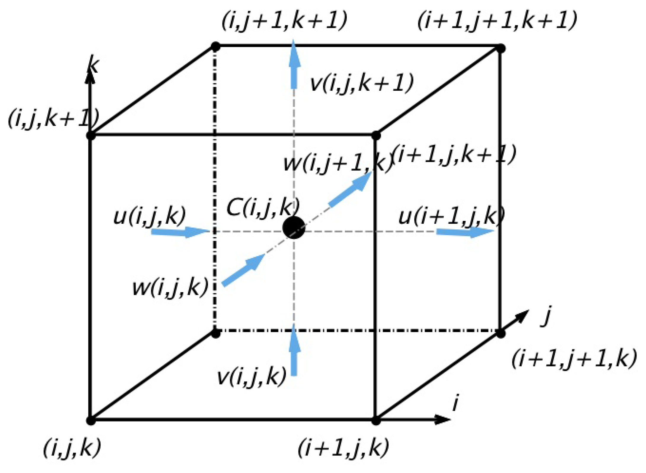
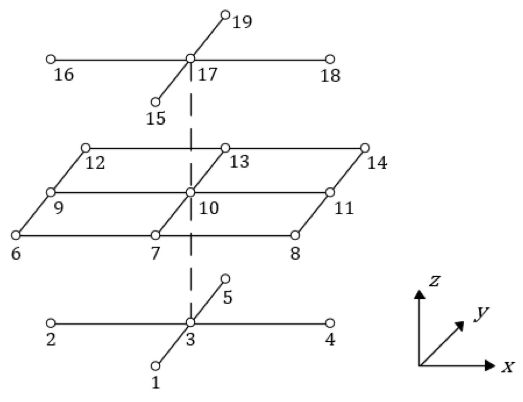
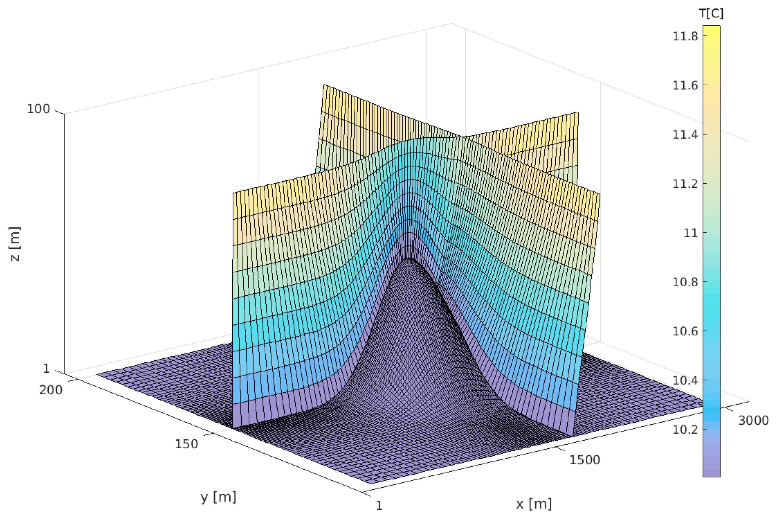
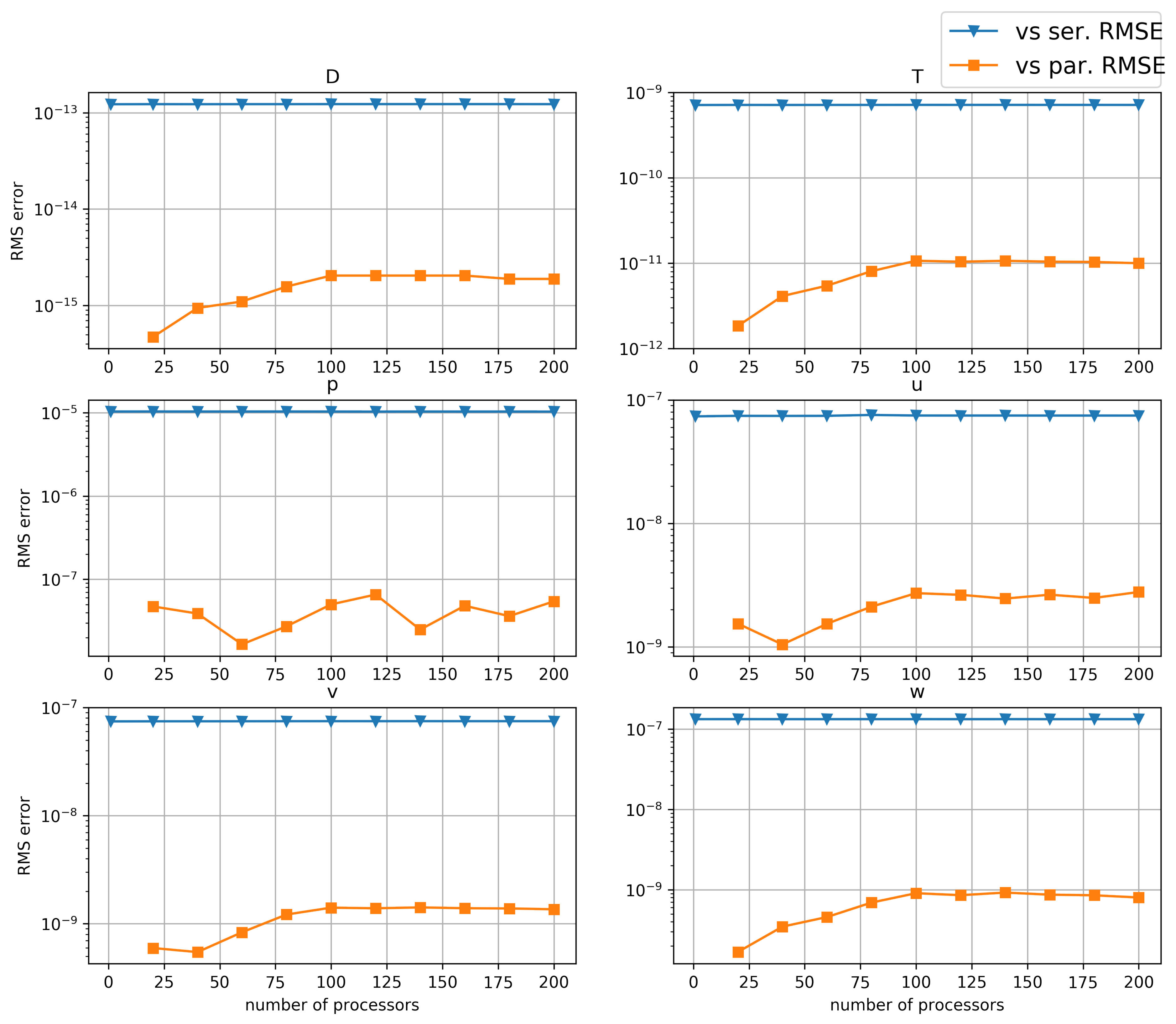
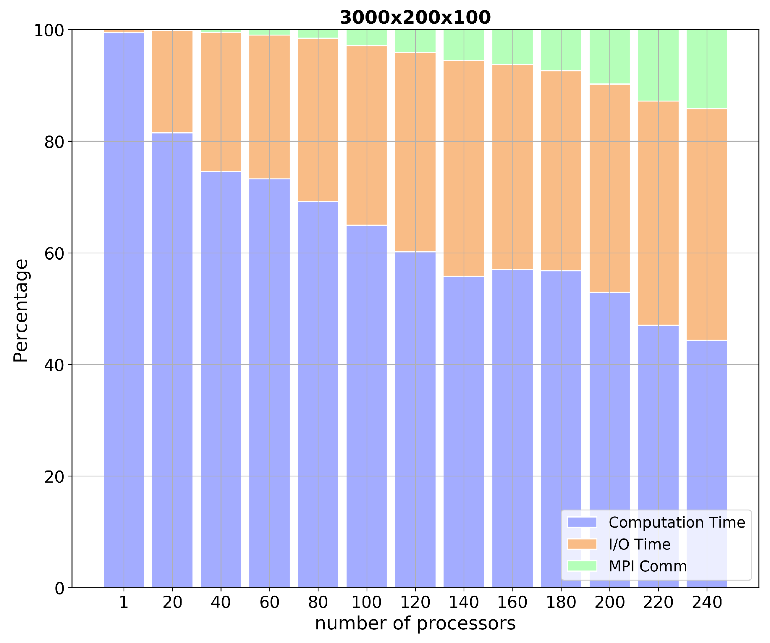
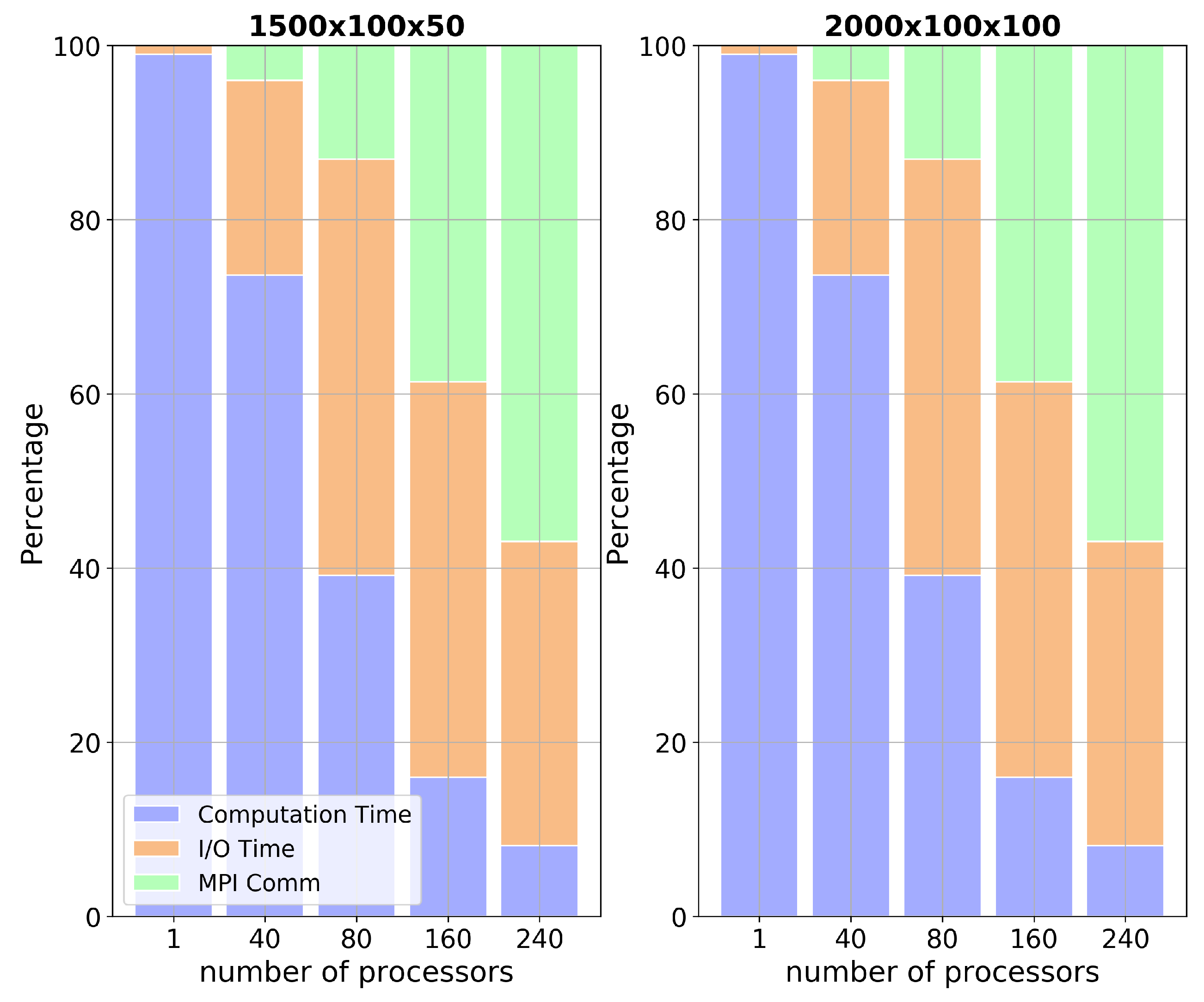
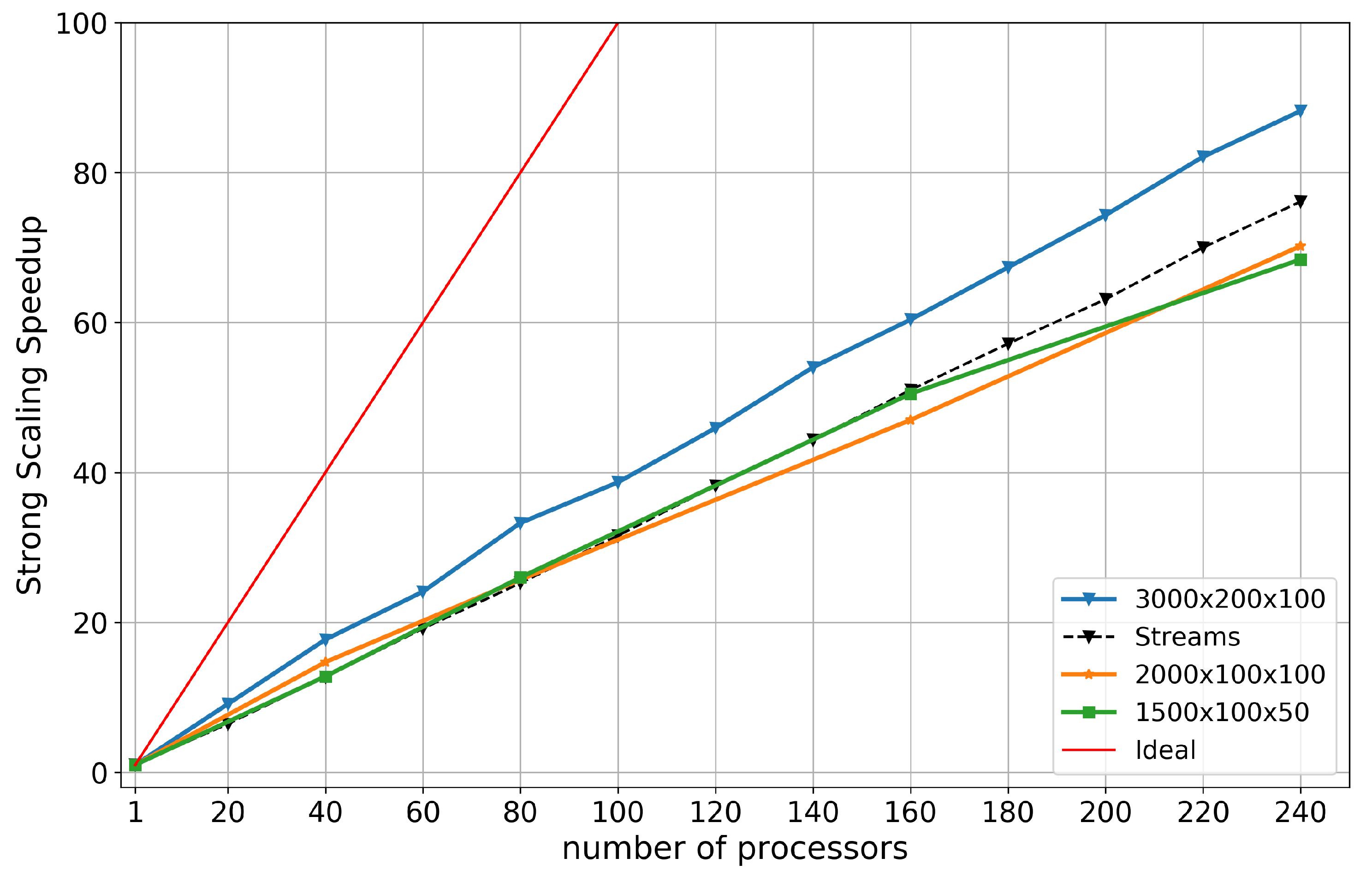
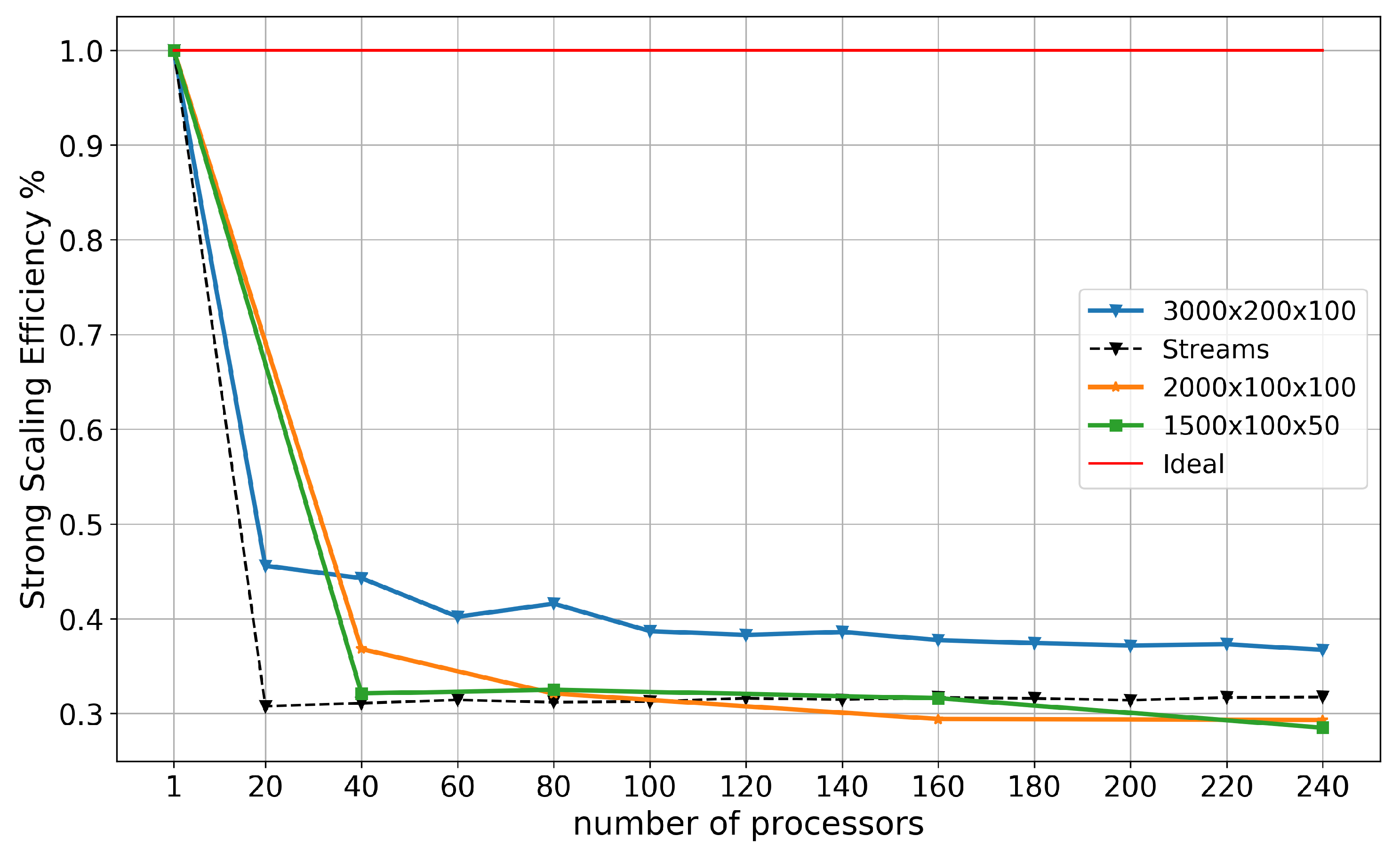
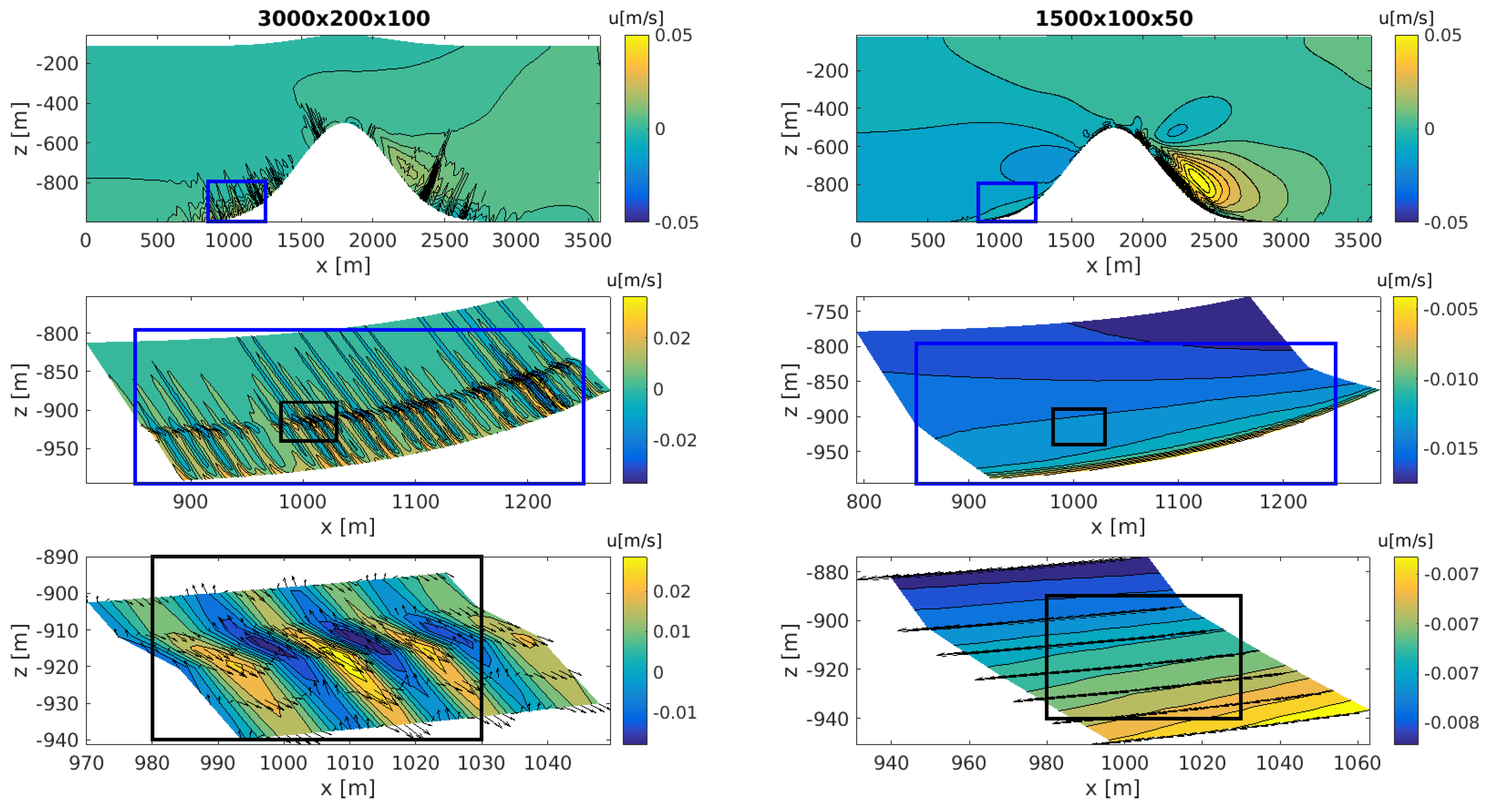
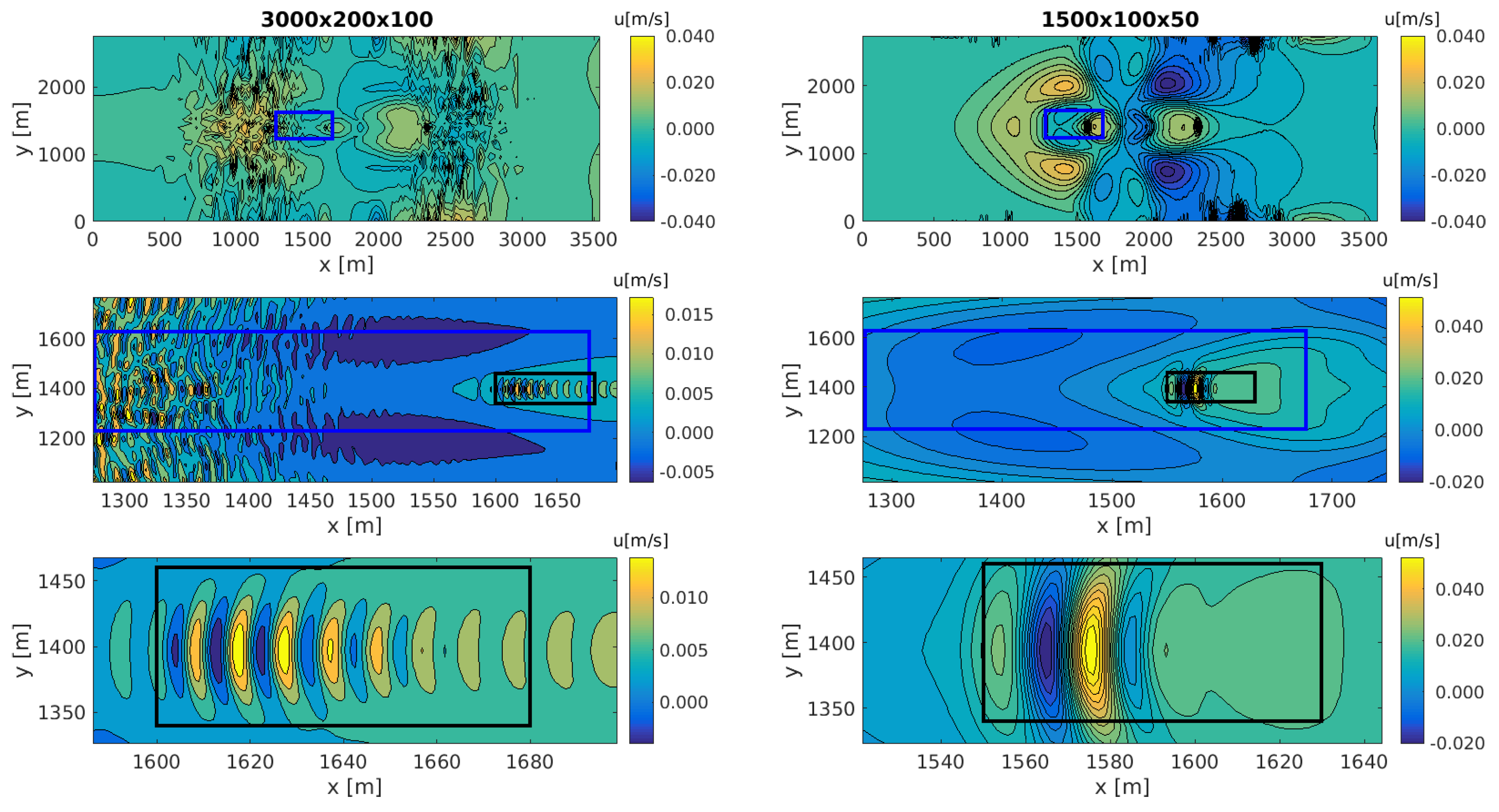


