1. Introduction
At the present time, one of the rapidly developing fields is mathematical modelling of water areas of particular interest (seas, bays, open ocean areas) and open coastal regions. The relevance of this topic is justified by the need to assess anthropogenic impacts on marine areas and the consequences of such impacts. Moreover, a number of problems connected to the climate changes for a selected water area over several decades gain increasing interest. In order to simulate coastal ocean processes, involved with various types of physical phenomena occurring at a wide range of spatial and temporal scales, special approaches are required. To provide the correct representation of coastal ocean flows, regional models are created.
Regional ocean modelling has one unavoidable challenge relative to its global counterpart: open boundary conditions (OBC). By definition, a regional ocean model includes open boundaries over at least a part of its perimeter [
1]. The “outer liquid” (open) boundary means the “water-to-water” boundary separating the considered area from an ocean. The result obtained both in long-term simulations and in operational forecasting directly depends on the method of setting the OBC. According to [
2], in flow problems dominated by advection and/or wave motion, the OBC should allow phenomena generated in the domain of interest and coming from outside to pass through the boundary without undergoing significant distortion and without influencing the interior solution. One of the difficulties in setting such conditions is that there is no accurate information on external energy and mass flows. If open boundaries are located in dynamically active areas, inaccurate accounting for this information leads to inconsistency of the results obtained with the observed fields of physical parameters. For the long-term climate modelling, the appropriate setting of boundary conditions at liquid boundaries is of particular importance.
There are different known methods [
3,
4,
5] dealing with open boundaries in limited-area models. In a number of studies [
6,
7] the models are previously set up for a larger area and the results of the preliminary (diagnostic) simulations with these models are used to determine OBC. One-way and two-way grid-nesting techniques are devised to exchange information at the interface between fine-mesh regional models and coarse-mesh large-domain models. The use of averaged data for flows across the open boundary is also acceptable in some cases [
8]. A large number of OBC have been proposed in the literature (see [
9], for a review). The adaptive algorithm described in [
3] is used in many recent studies. It is also possible to use sequential [
1] or variational [
5] data assimilation methods in order to reduce model-data misfit caused by unsatisfactory OBC. While there are many suggested methods, it is still a question of debate which methodology is suitable for a particular problem.
One of the approaches used for modelling multiphysics and multiscale coastal ocean processes is developing of hybrid models based on domain decomposition. The use of domain decomposition method (DDM) allows to reduce the solution process in the original domain to alternate solving the problem in subdomains, possibly having a simpler form, or apply different models in them (for example, the coupling of first and second order equations [
10]). Particularly, it is possible to use DDM to combine models developed for individual phenomena at specific scales. For example, in [
11,
12] the idea of coupling a geophysical fluid dynamics model and a fully 3D fluid dynamics model in order to simulate multiphysics coastal ocean flows is presented and discussed. Implementation of DDM often requires “inner liquid” boundaries, separating the subdomains. In these subdomains one can obtain the results of simulations using meshes of different scales to achieve better approximation of boundary, bottom topography, etc. At the present time, the development of new algorithms and their effective implementation on multiprocessor computer systems can be attributed to the main goals of the domain decomposition. This makes DDMs be promising in mathematical modelling of processes in the oceans and seas [
11,
12,
13]. Most studies on application of data assimilation (DA) together with DDM are related to developing parallel algorithms. Some studies [
14,
15,
16,
17] demonstrate the scalability of the domain decomposition approach and its mathematical consistency when applied in variational DA. Besides, DDM in variational DA problems is suitable not only for creating high-performance algorithms. Particularly, observational data could be available not in the whole modelling area but only in some subdomain in which variational DA procedure may be considered. In those cases the application of DDMs may be effective. This topic is a relatively new field in ocean modelling.
The approach described in this paper is based on [
13,
18,
19,
20,
21]. In [
18] the model based on primitive equations written in spherical
-coordinates with a free surface in the hydrostatic and Boussinesq approximations is considered. For time approximation of the model the splitting method is used [
22,
23]. For this purpose the whole time interval is divided into subintervals; at each subinterval, the following subproblems named the steps of the splitting method are solved:
Step 1. The heat transfer problem.
Step 2. The salt transport problem.
Step 3. The problem of hydrological fields adaptation. It is solved in 3 substeps: (a) calculation of density and finding corrections to the velocity; (b) solving the problem of baroclinic adaptation; (c) solving the problem of barotropic adaptation (i.e., the system of linearized shallow water equations is considered).
The steps of the splitting method are formulated in [
18]. The splitting method allows to consider the DA problem as a sequence of linear DA problems. In [
19,
20,
21,
24,
25] an investigation of some of them is given. In [
25] an iterative algorithm for solving the problem of variational assimilation of the temperature corresponding to the step 1 of the splitting method is considered. The numerical experiments on the efficiency of the algorithm in the Baltic Sea area are carried out. In [
19] an inverse problem of determining an unknown boundary function in the OBC for the simplest model of tides is studied. The results of the work are used in [
21], where the algorithm for solving the problem of variational assimilation of the sea level anomaly at the liquid boundary corresponding to step 3 of the splitting method is considered and tested in the Baltic Sea circulation model. In [
13] a new approach to formulation of DDM is discussed. This approach was applied to a convection-diffusion problem. The method described in [
13] was implemented in the heat transfer block (step 1) of the Baltic Sea dynamics model.
The purpose of this work is to apply DDM to the variational DA problem. The method for solving the problem of restoring boundary functions at the “outer” and “inner” liquid boundaries based on the methods of variational DA and domain decomposition for the subproblem corresponding to a system of linearized shallow water equations (step 3-c) is studied. The problem of determining additional unknowns (“boundary functions”) in the boundary conditions is considered as inverse and solved using well-known approaches [
26,
27]. The major problem in coastal ocean modelling is the reconciliation of model results with observational data. The approach described in the paper may be applied to regional ocean models in order to reduce a model-data misfit and the dependence of the results upon the unsatisfactory OBC. The choice of the approach to formulate the DDM in the present work is justified by a possibility of generalization, since the models in the subdomains may differ. Therefore, the results of this paper may be promising for multiscale and multiphysics coastal processes simulation.
2. Problem Statement
2.1. Notations and Preliminary Notes
Let us consider geographical (geodesic) system of coordinates (), where is the geographical longitude increasing from West to East, is the geographical latitude increasing form South to North (), r is the distance from the center of the Earth to a given point, the mean Earth radius is . Instead of r it is often convenient to introduce the coordinate of the axis , directed along the normal to the center of the sphere of radius , along the direction of the gravity force. The unit vectors in -, - and z-directions are denoted by , respectively. In this case the velocity vector in the ocean is written in the form: .
Let
denote the connected manifold on the sphere
, which is called the “reference surface” [
18]. Below we consider the case when
does not include polar points. The ocean surface elevation is given by the equation
,
is the bottom topography function, where (
,
,
,
[0,
T] is time variable (
T<
,
>0. Moreover, suppose that there exists
, so that
. Considering these notations, the total depth of the ocean is expressed as
Below we use the following notations of differential operators:
where
,
. By
we denote the unit vector of outer normal to
. Let
l
denote the Coriolis parameter,
g is the gravitational acceleration. Let us introduce the following notation for the depth-averaged horizontal velocities:
In the current study we consider the subproblem corresponding to a system of linearized shallow water equations (Step 3-c of the splitting scheme introduced above) on the time subinterval
,
,
,
,
[
18]:
where
is a given function,
is the linear drag coefficient. Solving the problem on
, we consider the functions
,
to be known. Detailed description of the notations and simplifications can be found, for example, in [
18]. In the present work we consider the boundary condition for System (
1) of the form [
19]:
where
is the characteristic function of the “outer liquid” (open) boundary
, i.e.,
if
,
otherwise. If the function
is defined, Systems (
1) and (
2) are well posed. This boundary function will be considered below as an additional unknown.
Considering Systems (
1) and (
2) on
, we introduce the following implicit scheme for time approximation:
Hereafter the “semi-discrete” System (
3) is the subject of the investigation, so for convenience the indices
j will be omitted, i.e.:
,
, ... We also introduce vectors
,
,
. Finally, System (
3) can be written in the form:
2.2. Variational Data Assimilation and the Domain Decomposition Method
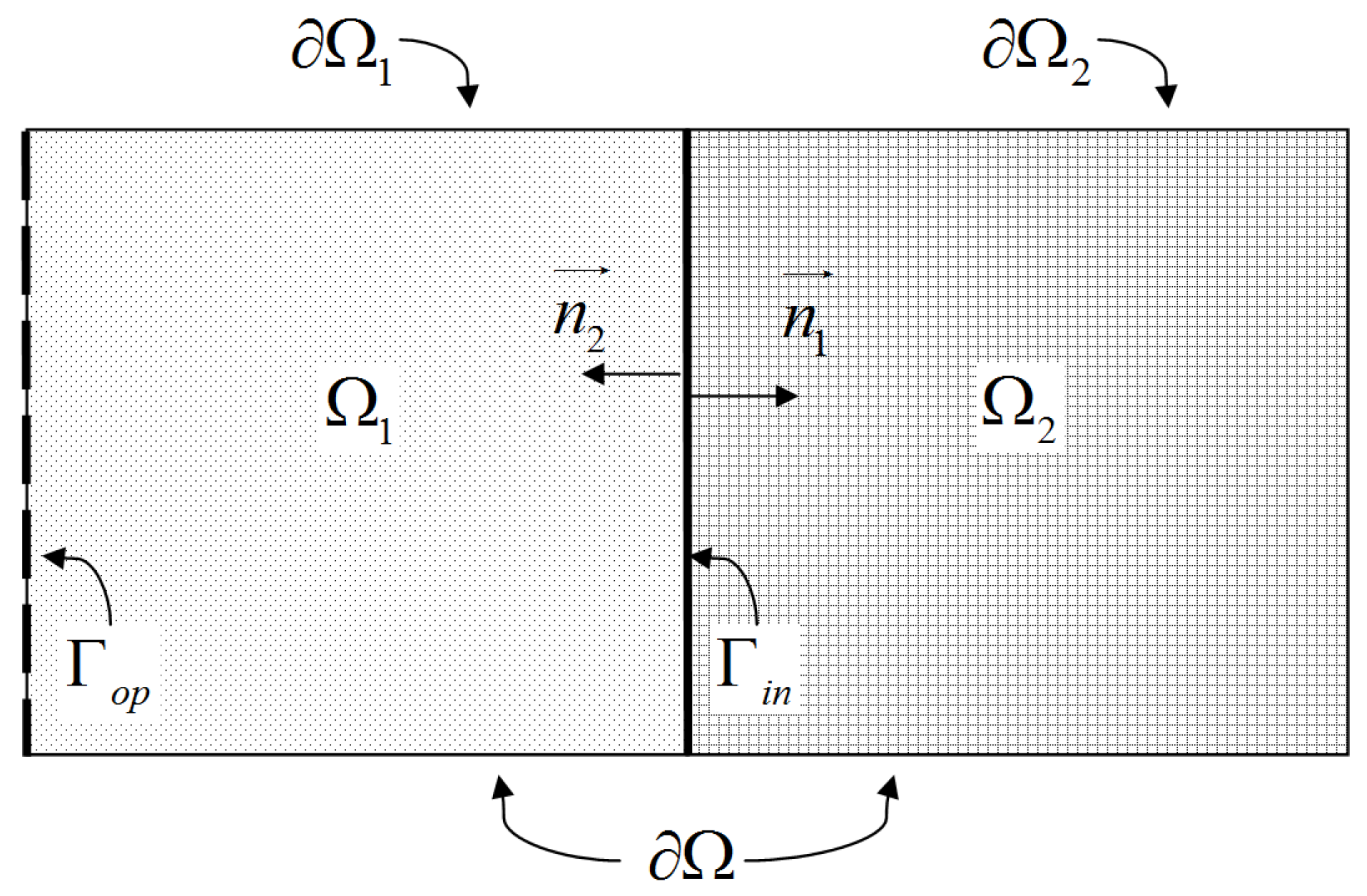
We assume that the boundary
of the domain
is Lipschitz and piecewise
–smooth. We also assume that
is a hypersurface of class
[
28] and divides the domain
into two subdomains
and
without overlap,
(see
Figure 1),
,
is open in
,
is open in
. We suppose that
and
are Lipschitz and piecewise
–smooth. Suppose that
(“outer liquid”, open boundary) does not intersect with
(“inner liquid” boundary). Moreover, the essential assumption is that
.
Below we use the index
to indicate the solutions in subdomains (
). The problem (
4) can be written for the functions
in the subdomain
, for the functions
in the subdomain
. Suppose
is the outer normal to the boundary
of the domain
,
. We will require the fulfillment of the boundary conditions on the inner liquid boundary
:
where
,
.
An additional unknown function
v is defined as:
We obtain the following form of the boundary conditions for the problem in the subdomain
:
and for the problem in the subdomain
:
Suppose there are preprocessed data of sea level anomaly measurements
along
. Such data can be obtained from observations or direct measurements (satellite altimetry data, “in-situ” data), or from the simulation using a global model with a coarser grid. In any cases, these data contain errors, so we cannot use
directly in the OBC. We introduce an additional condition (closure condition):
From System (
4) in each subdomain (
) we obtain:
We formulate the
inverse problem of restoring the boundary functions on the “outer” and “inner” liquid boundaries as follows: find the vector functions of solutions in the subdomains
,
, and additional unknown boundary functions
v,
, satisfying the systems of Equation (
9) and additional conditions of Equations (
5) and (
8).
Consider the Hilbert space
of vector functions
,
,
with the scalar product:
By we denote a space of vector functions . Let , , , .
The scalar product of (
9) and
in
,
is:
where
Let us introduce the Hilbert space of vector-functions , , , with the norm , where is the space of functions from with the “weighted” scalar product: . We also introduce the space .
We formulate the problem in a weak form: find
,
satisfying the conditions of Equations (
10) and (
11) and also the conditions of Equations (
5) and (
8) (in the sense of equality almost everywhere on
,
, respectively)
.
In order to formulate problems in operator form to study the problem theoretically the weak formulation should be modified. To execute this, we use the procedure similar to that described in [
19]. From Equation (
9) we receive:
where
By matrix
M we denote:
where
Substituting
in the weak formulation of the problem we receive:
where
Let us introduce the following notation:
The bilinear forms
,
are bounded and positive definite for functions
,
. Equations (
12) and (
13) can be formulated in the following form [
26]:
where the operators
,
,
(the space
is the dual of
) are introduced using the bilinear forms
,
,
,
, respectively [
29],
. The adjoint operators may also be introduced, so that the following identity is satisfied (
):
Note, that
,
and
means their scalar product. We obtain the same equalities for the bilinear forms
,
:
It could be shown that the operators
,
are bounded, there exist operators
which are bounded (
) [
13,
29].
The closure conditions of Equations (
5) and (
8) are formulated in the form:
where
is a trace operator on
,
,
,
, are trace operators on
,
.
Now the
weak formulation of the inverse problem is equivalent to the following: find
,
,
v satisfying Equations (
16), (17), (
20) and (21).
The system of Equations (
16), (17), (
20) and (21) can be rewritten in the operator form:
where
Finally, the original problem is reduced to a single operator Equation (
22), for which many results of the general theory of operator equations [
26,
27,
30] are applicable. In the current study the methodology based on the methods of optimal control and adjoint equations is used [
26].
2.3. Optimal Control Problem
Note that the operator
A is bounded:
,
. However Equation (
22) may be ill-posed, since the non-smooth observational data
are used in setting the function
, so
. In this regard let us move on to a
generalized formulation of Equation (22): find
minimizing
.
We formulate the class of optimal control problems [
26]: find boundary functions
, minimizing the functional
:
Note that the necessary condition for the minimum of the functional
has the form of an equation in terms of Tikhonov regularization method, where
is a regularization parameter. Henceforth, we will call
the
regularization parameter. If
, functional defined in Equation (
23) is strictly convex, strongly convex and has a unique global minimum
. If
and the solution of the inverse problem is unique,
tends to the solution when
. Note also that for
the optimal control problem is equivalent to the generalized formulation of Equation (
22).
4. Optimality Condition
The necessary optimality condition for the functional
can be written in the form:
where
is the adjoint to
A:
Introduce the following adjoint problem:
The optimality Equation (
24) takes the form:
We compute the scalar product of vector function
and Equation (
27) in
. Using Equations (
14) and (
15) and representations of the bilinear forms of Equation (
19), we receive the integral analogue of the optimality Equation (
27):
Similarly, integral relations for adjoint Equations (
25) and (26) can be obtained.
Adjoint Equations (
25) and (26) in differential form (
,
) are given by:
The optimality conditions take the form:
So, the functions
,
v minimizing
,
, satisfy the optimality Equations (
29) and (30), where
,
are the weak solutions of Equation (
28),
, in which
are the weak solutions of the systems of Equation (
9).
6. Iterative Algorithm
As it was shown in the
Section 3 and
Section 5, the problem to find
,
and the additional boundary functions
v,
is uniquely and densely solvable. Therefore the functions
,
,
satisfying Equations (
9) and (
28)–(30) could be taken as an approximation to the solution of the original problem [
26]. An approximation to
,
,
could be found with the following iterative algorithm.
1. Let
be found. Solve the problems in each subdomain
,
:
2. Solve the adjoint problems in
,
:
3. Find new
by:
Using assertions of [
26] we obtain the validity of the following theorem:
Theorem 1. (I) If – exact data, – measured data of observations (possibly containing errors), , , and are the solutions of the optimality systems of Equations (9) and (28)–(30), , then the following assessment is valid:where , . (II) If , then the inverse problem of Equation (22) has a unique normal solution . In that case for enough small vector function tends to in , when , . When the stopping criterion of iterative algorithm is satisfied, the functions
,
,
,
are taken as an approximate solution of the considered Equations (
5), (
8) and (
9) in
,
. Suitable stopping criterion should be chosen depending on the iterative parameters of the algorithm, size of the modelled region, numerical method, and a given accuracy. More often it is chosen as a limitation of iterations or of residual value. Equations (
31)–(34) converge for the small enough parameter
. However,
may be chosen as follows [
26]:
This choice of the parameter could be helpful to reduce the number of iterations required.
7. Numerical Experiments and Discussion
The described approach to domain decomposition and variational DA is applied to the system of shallow water systems of Equation (
4). Here
is a domain on the plane, and
are Cartesian coordinates. To set initial conditions, a preliminary calculation without the domain decomposition and variational DA methods is carried out. In this case the domain is represented by the rectangular
with
m. The value of the physical parameters are
m/
,
,
and
(m). The forces
and
are equal to 0. The boundary conditions are
. For this preliminary problem the conditions at
are given by (
p is a subscript for the preliminary results):
To discretize in time, an implicit scheme is used. The time step is 0.5 s. The finite difference method with the first order space discretization is applied. The spatial grid is uniform, the spatial grid steps are 1 m. The results of simulation after 25 s are taken as initial conditions to the next series of numerical experiments.
To set the observational data on , the preliminary experiment is continued on the next 5 s. At each time step after the first 25 s the observational data are chosen as , where a and b are random numbers in the range . The numbers are received by pseudo-random generators for the uniform distribution law. Thus, the obtained observational data are artificially noisy (noise level is ).
So, we get the initial conditions and the observational data for the next experiments with previously described approach of application of DA and DDMs.
For the numerical experiments the domain is the square . It is decomposed into the two subdomains and without overlap. We denote the “inner” boundary by and the “outer” boundary by . Here m. The value of the physical parameters are m/, , . The depth of the modelling domain is (m). The forces and are equal to 0.
To discretize in time, an implicit scheme is chosen. The time step is 0.5 s. The finite difference method with the first order space discretization is applied. The spatial grid is uniform, with grid steps 1 m. The described algorithm of domain decomposition and variational DA is implemented at each time step.
Table 1 gives the residual value depending on the noise level and the stopping criterion (the number of iterations less than 10 or less than 50). The residual value here is defined by
From
Table 1 one can see that the noise level has a significant impact on the residual value at the 50th iteration and has almost no affect at the 10th iteration.
Further in this section the stopping criterion is the number of iterations less than 50.
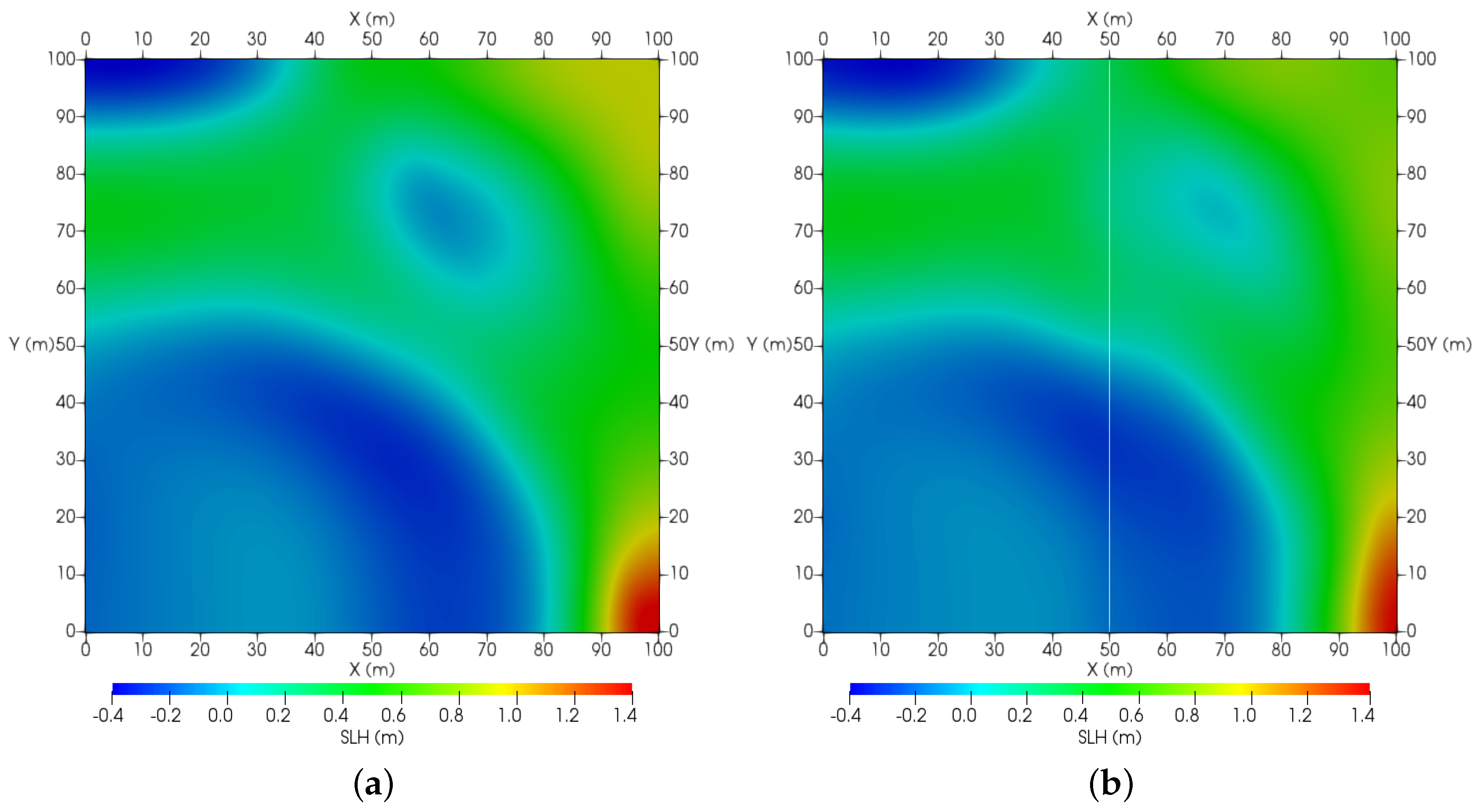
Figure 2 shows the results of modelling for the preliminary problem and the results of modelling using domain decomposition and variational DA. The “inner” boundary is presented as a white line. As seen in
Figure 2a,b, the results differ from each other. It is connected with the application of variational DA on the open boundary, because the observational data
used as closure condition Equation (
8) have some additional noise and the results reproduce it (as can be seen in
Figure 3).
The iterative algorithm converges with the chosen parameter
from Equation (
36).
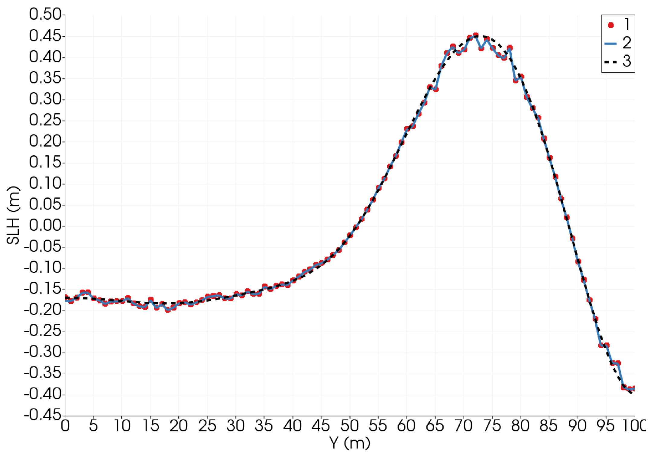
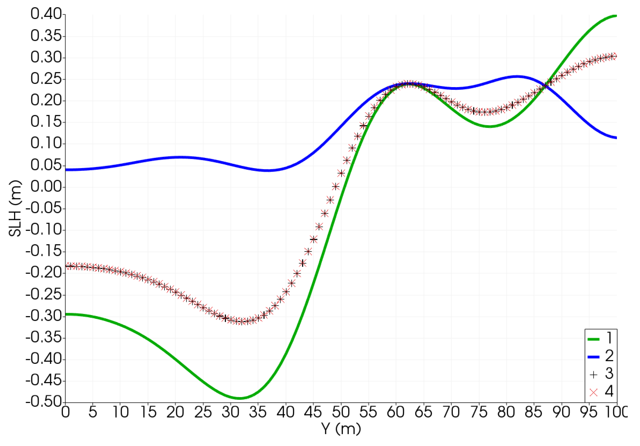
Figure 4 shows the results of sea level functions at the first, the ninth and the last iterations. For clarity, the observational data are also presented.
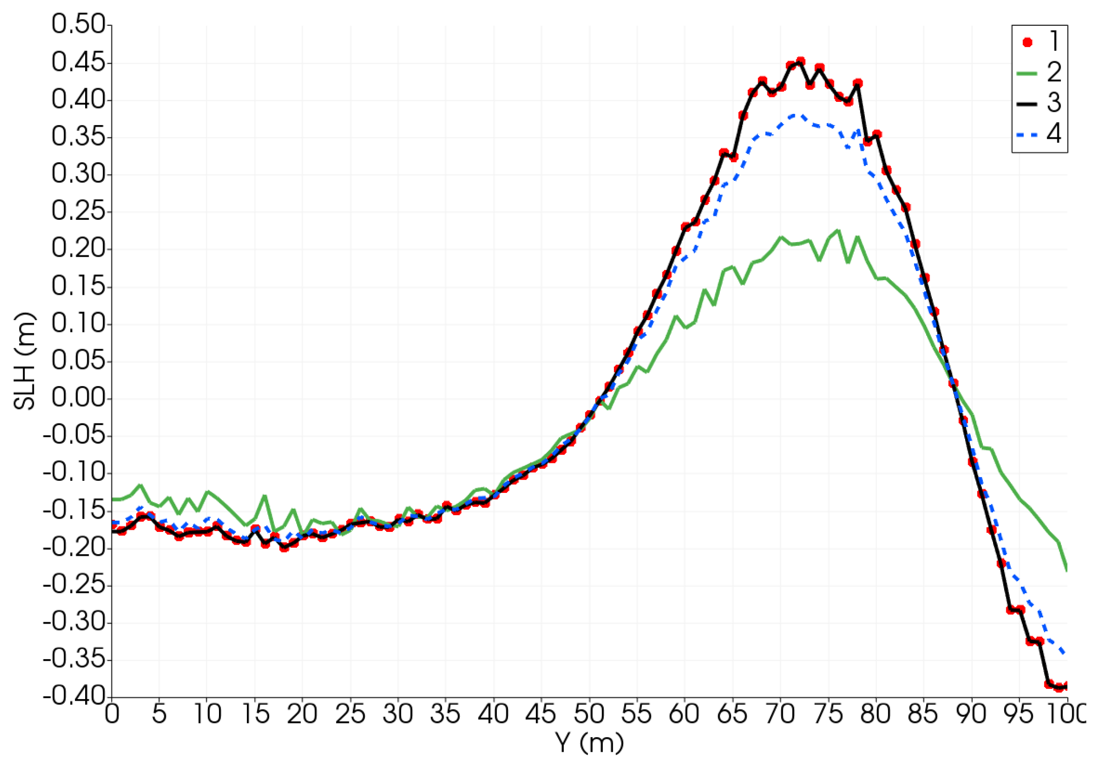
In order to analyse the impact on the simulation results of the DDM, the comparison of sea level function results at the first and the last iterations on
is presented in
Figure 5. We could note that
almost coincides with
on the “inner” boundary at the last iteration.
In addition, we study the dependence on the regularization parameter
. According to the theory [
27], an increase in the regularization parameter
leads to a decrease in the influence of additional noise on the solution.
Table 2 provides the error
depending on the regularization parameter
and the stopping criterion (the number of iterations less than 10 or less than 50). As expected, the error increases at the beginning, because the accuracy of the method is not sufficient to reproduce the additional noise (see
Figure 4 and
Table 1). When the stopping criterion is the number of iterations less than 50, the regularization parameter smooth the result.
Thus, application of DDMs in variational DA problem is considered. The time required to solve DA problem with using DDM slightly increases (by 5%) in contrast to one required to solve only DA procedure. The developing of a parallel algorithm based on the described approach may decrease the computation time.
8. Conclusions
The algorithm of DDM in the problem of variational DA is considered. The theoretical study of the problem has been carried out, including the study of the unique and dense solvability of the inverse problem. The iterative algorithm is proposed and the theorem concerning its convergence has been formulated. To illustrate the theoretical results the numerical experiments for the linearized shallow water equations have been carried out. The results of the numerical experiments show that the iterative algorithm converges with the parameter described in this paper. The DDM does not significantly affect the modelling results. The result of the simulation with variational DA method fits the observational data. However, the additional noise in the observational data yields a noise in the solution results. Experiments show that the effect of a noise may be mitigated by the regularisation. It is worth to be noted that the regularisation parameter and the iteration parameter should be chosen depending on a problem to be solved. These parameters affect the accuracy, convergence and rate of convergence.
In this paper we focus on the theoretical study of the inverse problem for the linearized system of shallow water equations. To illustrate the theoretical results the simplified example was considered. To estimate the approach, its quality and the possibility of application to realistic problems, more experimental results should be provided. We are going to continue the study and test the algorithm in the regional ocean models (e.g., [
22,
31]). In this case the algorithm will be implemented at each time step to the problem corresponding to step 3-c of the splitting method (mentioned in
Section 1). The general approach outlined here may be extended to other regional ocean models. However, for each special problem, boundary conditions on the inner and outer liquid boundaries should be formulated depending on chosen simplifications and the corresponding theoretical study should be carried out. It is worth noting that the methodology based on the theory of optimal control and adjoint equations (used in this paper) may be applied to nonlinear problems. In addition, it may become possible to use meshes of different scales in subdomains. Moreover, the general approach may be improved to become suitable for modelling multiphysics and multiscale coastal ocean processes.


