Sediment Transport Processes during Barrier Island Inundation under Variations in Cross-Shore Geometry and Hydrodynamic Forcing


Abstract
:1. Introduction
2. Methods
2.1. Model Description
2.1.1. Hydrodynamic Model—SWASH
2.1.2. Sediment Transport Model
2.2. Model Implementations and Experiment Set-Up
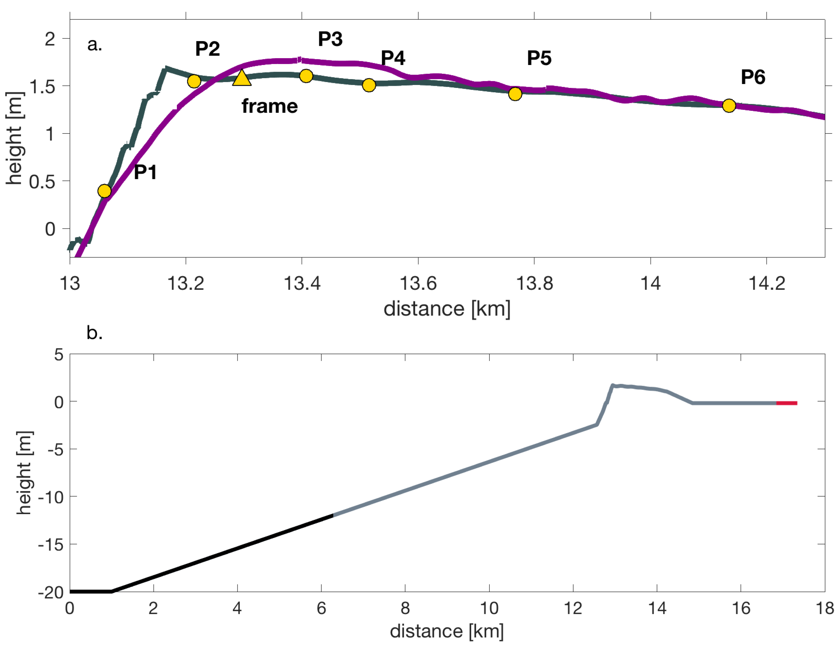
2.2.1. Field Observations
2.2.2. Boundary Conditions
2.2.3. Introduction of Scenarios for SWASH Computations
3. Results
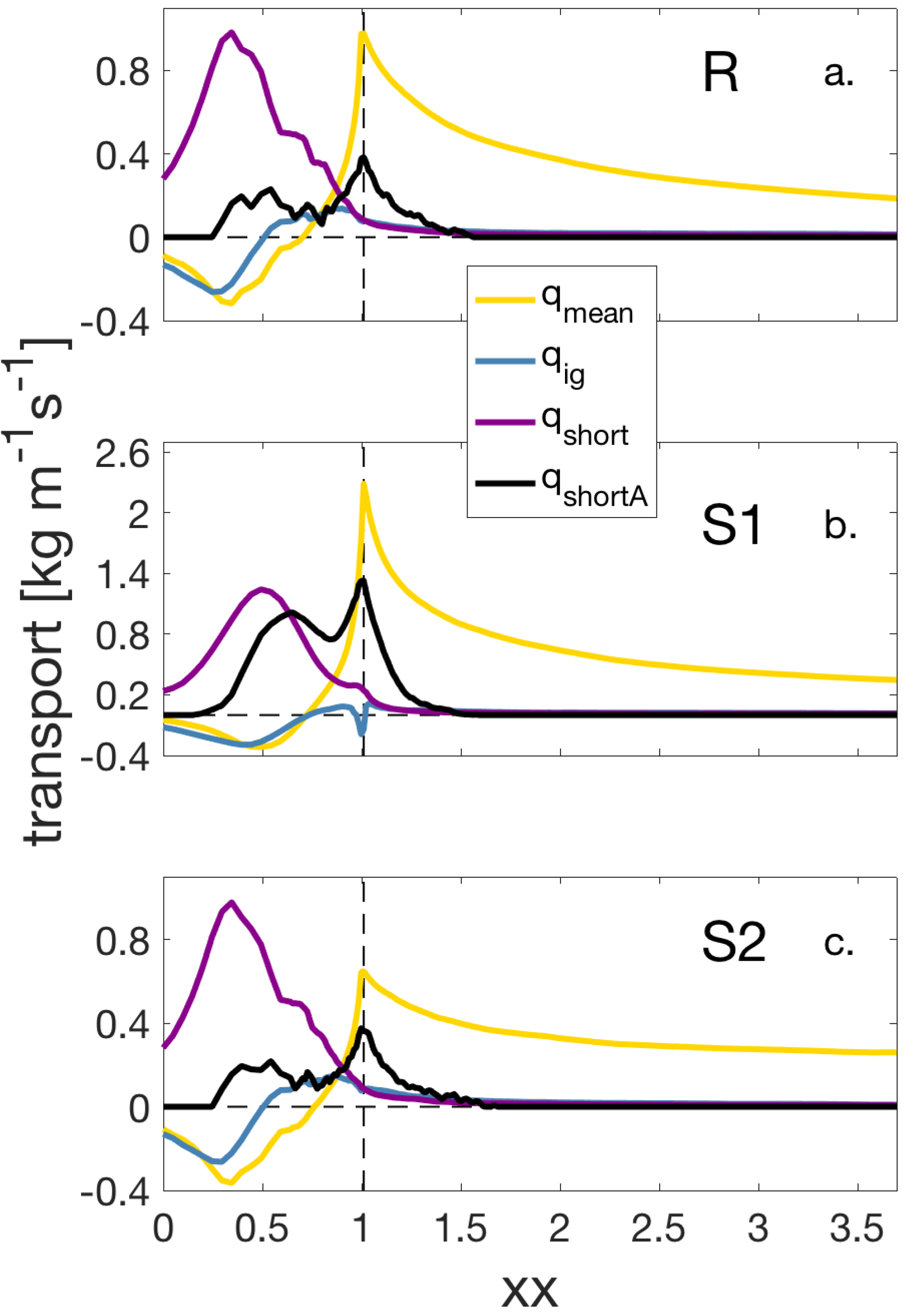
3.1. Reference Case
3.2. Slope Comparisons
3.3. Variations in Hydrodynamic Forcing and Inundation Depths
4. Discussion
4.1. Role of Waves and Mean Flow throughout the Domain
4.2. Implications for Barrier Islands
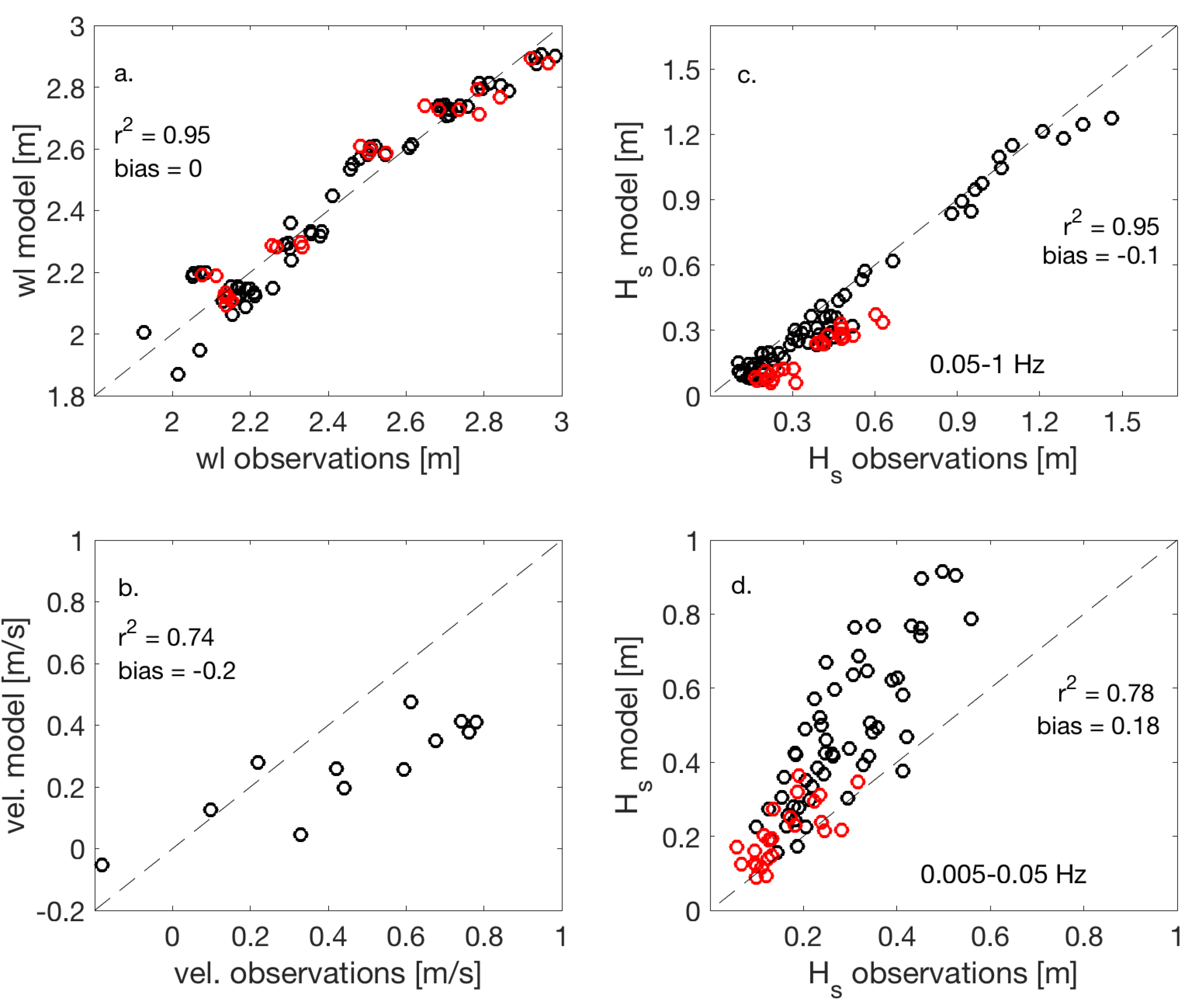
4.3. Model Performance and Sensitivity of Results to Model Implementations
5. Conclusions
Author Contributions
Funding
Acknowledgments
Conflicts of Interest
Appendix A
Appendix A.1. Boundary Conditions and Model Settings

| Flooding | Wind | Wind | Wave | Wave | Wave | Water Level | Water Level |
|---|---|---|---|---|---|---|---|
| Speed | Direction | Hs | T | N. Sea | W. Sea | ||
| # | [m/s] | [] | [m] | [s] | [] | [m] | [m] |
| 1 | 16 | 270 | 6.20 | 8.7 | 307 | 2.34 | 2.52 |
| 2 | 11 | 300 | 5.11 | 8.3 | 327 | 1.84 | 2.19 |
| 3 | 15 | 310 | 4.55 | 7.2 | 321 | 2.05 | 2.16 |
| 4 | 20 | 330 | 7.43 | 10.1 | 326 | 2.50 | 2.92 |
Appendix A.2. Model-Data Comparison


References
- Donnelly, C.; Kraus, N.; Larson, M. State of Knowledge on Measurement and Modeling of Coastal Overwash. J. Coast. Res. 2006, 22, 965–991. [Google Scholar] [CrossRef]
- Sallenger, A.H., Jr. Storm impact scale for barrier islands. J. Coast. Res. 2000, 16, 890–895. [Google Scholar] [CrossRef]
- Safak, I.; Warner, J.C.; List, J.H. Barrier island breach evolution: Alongshore transport and bay-ocean pressure gradient interactions. J. Geophys. Res. Oceans 2016, 121, 8720–8730. [Google Scholar] [CrossRef]
- Durán, R.; Guillén, J.; Ruiz, A.; Jiménez, J.A.; Sagristà, E. Morphological changes, beach inundation and overwash caused by an extreme storm on a low-lying embayed beach bounded by a dune system (NW Mediterranean). Geomorphology 2016, 274, 129–142. [Google Scholar] [CrossRef] [Green Version]
- Donnelly, C. Morphologic Change by Overwash: Establishing and Evaluating Predictors. J. Coast. Res. 2007, 23, 520–526. [Google Scholar]
- Rosati, J.; Stone, G.W. Critical Width of Barrier Islands and Implications for Engineering Design. In Proceedings of the Sixth International Symposium on Coastal Engineering and Science of Coastal Sediment Process, New Orleans, LA, USA, 13–17 May 2007; pp. 1–14. [Google Scholar] [CrossRef]
- Engelstad, A.; Ruessink, B.G.; Hoekstra, P.; van der Vegt, M. Sand Suspension and Transport During Inundation of a Dutch Barrier Island. J. Geophys. Res. Earth Surf. 2018, 123, 3292–3307. [Google Scholar] [CrossRef] [Green Version]
- Engelstad, A.; Ruessink, B.; Wesselman, D.; Hoekstra, P.; Oost, A.; van der Vegt, M. Observations of waves and currents during barrier island inundation. J. Geophys. Res. Oceans 2017, 122, 3152–3169. [Google Scholar] [CrossRef] [Green Version]
- Sherwood, C.R.; Long, J.W.; Dickhudt, P.J.; Dalyander, P.S.; Thompson, D.M.; Plant, N.G. Inundation of a barrier island (Chandeleur Islands, Louisiana, USA) during a hurricane: Observed water-level gradients and modeled seaward sand transport. J. Geophys. Res. Earth Surf. 2014, 119, 1498–1515. [Google Scholar] [CrossRef]
- Harter, C.; Figlus, J. Numerical modeling of the morphodynamic response of a low-lying barrier island beach and foredune system inundated during Hurricane Ike using XBeach and CSHORE. Coast. Eng. 2017, 120, 64–74. [Google Scholar] [CrossRef]
- Hoekstra, P.; ten Haaf, M.; Buijs, P.; Oost, A.; Klein Breteler, R.; van der Giessen, K.; van der Vegt, M. Washover development on mixed-energy, mesotidal barrier island systems. Coast. Dyn. 2009, 83, 25–32. [Google Scholar] [CrossRef]
- Wesselman, D.; Winter, R.; Engelstad, A.; McCall, R.; Dongeren, A.; Hoekstra, P.; Oost, A.; Vegt, M. The effect of tides and storms on the sediment transport across a Dutch barrier island. Earth Surf. Process. Landf. 2017, 43, 579–592. [Google Scholar] [CrossRef] [Green Version]
- Van Dongeren, A.; Battjes, J.; Janssen, T.; Van Noorloos, J.; Steenhauer, K.; Steenbergen, G.; Reniers, A.J.H.M. Shoaling and shoreline dissipation of low-frequency waves. J. Geophys. Res. Oceans 2007, 112. [Google Scholar] [CrossRef] [Green Version]
- De Bakker, A.T.M.; Tissier, M.F.S.; Ruessink, B.G. Shoreline dissipation of infragravity waves. Cont. Shelf Res. 2014, 72, 73–82. [Google Scholar] [CrossRef]
- De Bakker, A.T.M.; Brinkkemper, J.A.; van der Steen, F.; Tissier, M.F.S.; Ruessink, B.G. Cross-shore sand transport by infragravity waves as a function of beach steepness. J. Geophys. Res. Earth Surf. 2016, 121, 1786–1799. [Google Scholar] [CrossRef]
- Ruessink, B.G.; Kleinhans, M.G.; den Beukel, P.G.L. Observations of swash under highly dissipative conditions. J. Geophys. Res. Oceans 1998, 103, 3111–3118. [Google Scholar] [CrossRef]
- Stockdon, H.F.; Holman, R.A.; Howd, P.A.; Sallenger, A.H. Empirical parameterization of setup, swash, and runup. Coast. Eng. 2006, 53, 573–588. [Google Scholar] [CrossRef]
- de Bakker, A.T.M.; Tissier, M.F.S.; Ruessink, B.G. Beach steepness effects on nonlinear infragravity-wave interactions: A numerical study. J. Geophys. Res. Oceans 2015, 121, 554–570. [Google Scholar] [CrossRef]
- Rosati, J.D.; Stone, G.W. Geomorphologic Evolution of Barrier Islands along the Northern U.S. Gulf of Mexico and Implications for Engineering Design in Barrier Restoration. J. Coast. Res. 2009, 25, 8–22. [Google Scholar] [CrossRef]
- Schupp, C.A.; Winn, N.T.; Pearl, T.L.; Kumer, J.P.; Carruthers, T.J.; Zimmerman, C.S. Restoration of overwash processes creates piping plover (Charadrius melodus) habitat on a barrier island (Assateague Island, Maryland). Estuar. Coast. Shelf Sci. 2013, 116, 11–20. [Google Scholar] [CrossRef]
- Zijlema, M.; Stelling, G.; Smit, P. SWASH: An operational public domain code for simulating wave fields and rapidly varied flows in coastal waters. Coast. Eng. 2011, 58, 992–1012. [Google Scholar] [CrossRef]
- Rijnsdorp, D.P.; Smit, P.B.; Zijlema, M. Non-hydrostatic modelling of infragravity waves under laboratory conditions. Coast. Eng. 2014, 85, 30–42. [Google Scholar] [CrossRef]
- Smit, P.; Janssen, T.; Holthuijsen, L.; Smith, J. Non-hydrostatic modeling of surf zone wave dynamics. Coast. Eng. 2014, 83, 36–48. [Google Scholar] [CrossRef]
- Rijnsdorp, D.P.; Ruessink, G.; Zijlema, M. Infragravity-wave dynamics in a barred coastal region, a numerical study. J. Geophys. Res. Oceans 2015, 120, 4068–4089. [Google Scholar] [CrossRef]
- Fiedler, J.W.; Smit, P.B.; Brodie, K.L.; McNinch, J.; Guza, R.T. Numerical modeling of wave runup on steep and mildly sloping natural beaches. Coast. Eng. 2018, 131, 106–113. [Google Scholar] [CrossRef]
- Rijnsdorp, D.; Smit, P.; Zijlema, M. Non-hydrostatic modelling of infragravity waves using SWASH. Coast. Eng. Proc. 2012, 1, 27. [Google Scholar] [CrossRef]
- Guza, R.T.; Feddersen, F. Effect of wave frequency and directional spread on shoreline runup. Geophys. Res. Lett. 2012, 39, L11607. [Google Scholar] [CrossRef]
- Bagnold, R.A. An Approach to the Sediment Transport Problem from General Physics. U.S. Geol. Surv. Prof. Pap. 1966, 422-I. [Google Scholar] [CrossRef]
- Bailard, J.A. An energetics total load sediment transport model for a plane sloping beach. J. Geophys. Res. Oceans 1981, 86, 10938–10954. [Google Scholar] [CrossRef]
- Drake, T.G.; Calantoni, J. Discrete particle model for sheet flow sediment transport in the nearshore. J. Geophys. Res. Oceans 2001, 106, 19859–19868. [Google Scholar] [CrossRef]
- Hoefel, F.; Elgar, S. Wave-induced sediment transport and sandbar migration. Science 2003, 299, 1885–1887. [Google Scholar] [CrossRef] [PubMed]
- Smit, P.; Zijlema, M.; Stelling, G. Depth-induced wave breaking in a non-hydrostatic, near-shore wave model. Coast. Eng. 2013, 76, 1–16. [Google Scholar] [CrossRef]
- Thornton, E.B.; Humiston, R.T.; Birkemeier, W. Bar/trough generation on a natural beach. J. Geophys. Res. Oceans 1996, 101, 12097–12110. [Google Scholar] [CrossRef]
- Gallagher, E.L.; Elgar, S.; Guza, R. Observations of sand bar evolution on a natural beach. J. Geophys. Res. Oceans 1998, 103, 3203–3215. [Google Scholar] [CrossRef] [Green Version]
- Ruessink, B.G.; Houwman, K.T.; Hoekstra, P. The systematic contribution of transporting mechanisms to the cross-shore sediment transport in water depths of 3 to 9 m. Mar. Geol. 1998, 152, 295–324. [Google Scholar] [CrossRef]
- Janssen, T.T.; Battjes, J.A.; van Dongeren, A.R. Long waves induced by short-wave groups over a sloping bottom. J. Geophys. Res. Oceans 2003, 108, 3252. [Google Scholar] [CrossRef]
- Tissier, M.; Bonneton, P.; Michallet, H.; Ruessink, B.G. Infragravity-wave modulation of short-wave celerity in the surf zone. J. Geophys. Res. Oceans 2015, 120, 6799–6814. [Google Scholar] [CrossRef]
- Symonds, G.; Black, K.P.; Young, I.R. Wave-driven flow over shallow reefs. J. Geophys. Res. 1995, 100, 2639. [Google Scholar] [CrossRef]
- Aagaard, T.; Greenwood, B.; Hughes, M. Sediment transport on dissipative, intermediate and reflective beaches. Earth-Sci. Rev. 2013, 124, 32–50. [Google Scholar] [CrossRef]
- Butt, T.; Russell, P. Suspended sediment transport mechanisms in high-energy swash. Mar. Geol. 1999, 161, 361–375. [Google Scholar] [CrossRef]
- Aagaard, T.; Greenwood, B. Suspended sediment transport and the role of infragravity waves in a barred surf zone. Mar. Geol. 1994, 118, 23–48. [Google Scholar] [CrossRef]
- Goff, J.A.; Allison, M.A.; Gulick, S.P.S. Offshore transport of sediment during cyclonic storms: Hurricane Ike (2008), Texas Gulf Coast, USA. Geology 2010, 38, 351–354. [Google Scholar] [CrossRef]
- Elgar, S.; Gallagher, E.L.; Guza, R.T. Nearshore sandbar migration. J. Geophys. Res. Oceans 2001, 106, 11623–11627. [Google Scholar] [CrossRef]
- Ruessink, B.G.; van den Berg, T.J.J.; van Rijn, L.C. Modeling sediment transport beneath skewed asymmetric waves above a plane bed. J. Geophys. Res. Oceans 2009, 114, C11021. [Google Scholar] [CrossRef]
- Brinkkemper, J.A.; Aagaard, T.; de Bakker, A.T.M.; Ruessink, B.G. Shortwave Sand Transport in the Shallow Surf Zone. J. Geophys. Res. Earth Surf. 2018, 123, 1145–1159. [Google Scholar] [CrossRef] [PubMed]
- Grasso, F.; Michallet, H.; Barthelemy, E. Sediment transport associated with morphological beach changes forced by irregular asymmetric, skewed waves. J. Geophys. Res. Oceans 2011, 116. [Google Scholar] [CrossRef] [Green Version]
- Ruessink, B.G.; Michallet, H.; Abreu, T.; Sancho, F.; Van der A, D.A.; Van der Werf, J.J.; Silva, P.A. Observations of velocities, sand concentrations, and fluxes under velocity-asymmetric oscillatory flows. J. Geophys. Res. Oceans 2011, 116, C03004. [Google Scholar] [CrossRef]


| R | H | L | |||||
|---|---|---|---|---|---|---|---|
| (m) | 7.45 | 7.45 | 7.45 | 4.55 | 7.45 | 4.55 | 7.45 |
| (s) | 10.0 | 10.0 | 10.0 | 7.2 | 10.0 | 7.2 | 10.0 |
| wl N-Sea (m) | 2.5 | 2.5 | 2.5 | 2.5 | 2.5 | 2.5 | 2.0 |
| wl W-Sea (m) | 2.65 | 2.65 | 2.65 | 2.65 | 3.05 | 3.05 | 2.15 |
| seaward slope | 1:120 | 1:30 | 1:120 | 1:120 | 1:120 | 1:120 | 1:120 |
| landward slope | 1:2000 | 1:2000 | 0 | 1:2000 | 1:2000 | 1:2000 | 1:2000 |
© 2019 by the authors. Licensee MDPI, Basel, Switzerland. This article is an open access article distributed under the terms and conditions of the Creative Commons Attribution (CC BY) license (http://creativecommons.org/licenses/by/4.0/).
Share and Cite
Engelstad, A.; Ruessink, G.; Hoekstra, P.; van der Vegt, M. Sediment Transport Processes during Barrier Island Inundation under Variations in Cross-Shore Geometry and Hydrodynamic Forcing. J. Mar. Sci. Eng. 2019, 7, 210. https://doi.org/10.3390/jmse7070210
Engelstad A, Ruessink G, Hoekstra P, van der Vegt M. Sediment Transport Processes during Barrier Island Inundation under Variations in Cross-Shore Geometry and Hydrodynamic Forcing. Journal of Marine Science and Engineering. 2019; 7(7):210. https://doi.org/10.3390/jmse7070210
Chicago/Turabian StyleEngelstad, Anita, Gerben Ruessink, Piet Hoekstra, and Maarten van der Vegt. 2019. "Sediment Transport Processes during Barrier Island Inundation under Variations in Cross-Shore Geometry and Hydrodynamic Forcing" Journal of Marine Science and Engineering 7, no. 7: 210. https://doi.org/10.3390/jmse7070210