Article

Analysis of Hydrodynamic Performance of L-Type Podded Propulsion with Oblique Flow Angle

College of Shipbuilding Engineering, Harbin Engineering University, Harbin 150001, China
*
Author to whom correspondence should be addressed.
J. Mar. Sci. Eng. 2019, 7(2), 51; https://doi.org/10.3390/jmse7020051
Submission received: 23 January 2019 / Revised: 16 February 2019 / Accepted: 18 February 2019 / Published: 20 February 2019
(This article belongs to the Special Issue Marine Propulsion)

Abstract

:
In this study, the Reynolds-averaged Navier–Stokes (RANS) method and a model experimental test in a towing tank are used to investigate the unsteady hydrodynamic performance of L-type podded propulsion under different oblique flow angles and advance coefficients. The results show that the load of the operative propeller increases with oblique flow angle and the bracket adds resistance to the pod due to the impact of water flow, leading to a reduced propeller thrust coefficient with increased oblique flow angle. Under a high advance coefficient, the speed of increase of the pressure effect is higher than that of the viscosity effect, and the propeller efficiency increases with the oblique flow angle. The nonuniformity of the inflow results in varying degrees of asymmetry in the horizontal and vertical distributions of the propeller blade pressure. Under high oblique flow angle, relatively strong interference effects are seen between venting vortexes and the cabin after blades, leading to a disorderly venting vortex system after the blade. The numerical simulation results are in good agreement with the experimental values. The study findings provide a foundation for further research on L-type podded propulsors.

1. Introduction

Podded propulsion can be used to both propel and manipulate a ship, including rotating it horizontally by 360°. Compared to traditional propeller propulsion systems with a rudder, a podded propulsion system can operate beyond the design point during rotation and manipulation. Unlike in normal navigational states, the thrust and torque of podded propulsion and the propeller power will change at different deflection angles. Therefore, studies have been increasingly focusing on the hydrodynamic performance under such extreme operating conditions that were not considered during this design [1].
In recent years, viscous flow calculations have been widely used due to improvements in computing capabilities [2,3]. Researchers prefer the viscous flow method because it offers a more complete physical concept than the potential flow method. Chicherin et al. [4] conducted a preliminary analysis of scale-affected podded propulsors using Reynolds-averaged Navier–Stokes (RANS) equation and investigated the influences of different advance coefficients and Reynolds numbers on pods and struts; their results suggested that the scale factor was a more effective predictor of the resistance performance of propulsors than the shape factor. Ohashi et al. [5] studied the performance of a contrarotating podded propulsor with fore and aft propellers using RANS equations. They treated a propulsor pod unit with a detached propeller as a stern appendage; a comparison between calculated and test results showed that their method improved the calculation accuracy of ship resistance but worsened the prediction accuracy of the wake fraction and calculation accuracy of thrust deduction. Liu et al. [6] studied the unsteady hydrodynamic performance of podded propulsion under various deflection conditions and analyzed the changes in the propeller thrust, torque and pod steering torque with deflection angles. Amini et al. [7] used the RANS method and potential flow method to numerically calculate the bearing forces of a podded propulsion system under different deflection angles. Guo et al. [8] applied computational fluid dynamics (CFD) software to conduct steady and unsteady computational analyses of the hydrodynamic performance of a puller podded propulsor under an oblique navigational state. Zhou et al. [9] adopted the multireference quasisteady model, mixed surface steady model, and sliding grid unsteady model to perform simulation analyses of the hydrodynamic performance of podded propulsion under both direct and oblique navigational states. Xiong et al. [10] used the sliding grid method in combination with RANS equations and the Re-Normalization Group (RNG) k-ε turbulence model to conduct numerical simulations of the hydrodynamic performance of podded propulsion under a deflection state. A comparison and analysis of the experimental and numerical results showed that the deviation between the calculated and experimental values increased with the deflection angle, especially for large deviations of the thrust of podded propulsion along the incoming flow, but the overall trend was the same.
Previous experimental studies have used MARIN and HSVA tank tests to investigate the hydrodynamic performance of podded propulsors, and preliminary testing procedures for podded propulsors in open-water conditions have been established [11]. Reichel [12] tested a pusher podded propulsor with a right-handed propeller in a towing tank and analyzed the propulsor thrust and torque at various azimuthing angles. The results showed that the fluctuation of the side force on the propulsor during azimuthing conditions at an angle of ~15° to the right was greater than that at other yaw angles. The hydrodynamic characteristics of podded propulsors at a specific angle with the inflow at different advance coefficients were compared, and the thrust and side forces in left- and right-handed azimuthing conditions were also compared. At larger yaw angles, interactions between the propeller and pod showed more significant effects on the thrust and side forces on the podded propulsor. Islam et al. [13] conducted experiments with puller and pusher podded propulsors to investigate the effects of the hub taper angle on inflow, thrust, and efficiency; influence of pod and strut configurations; cavitation performance; effect of hub gap; and hydrodynamic performance of podded propulsor under static azimuthing conditions. They also conducted a preliminary analysis of factors affecting the experimental accuracy and provided some experimental guidance for research on podded propulsors under different azimuthing conditions. Furthermore, Islam et al. [14] compared the hydrodynamic characteristics of puller podded propulsors in static and dynamic azimuthing conditions and found that results varied primarily with rotations of the propeller and turning of the unit under dynamic azimuthing conditions. They then fitted a 10th-order polynomial model to the experimental results, which was similar to the hydrodynamic curve obtained for static azimuthing conditions. Palm et al. [15] conducted an experimental test and a CFD simulation to investigate variations in the hydrodynamic performance of cycloidal and pusher podded propulsors for straight-ahead motion at various draft depths. They discovered that the pusher podded propulsor was influenced to a greater degree by the draft and that the thrust linearly decreased as the draft decreased, whereas only a portion of the cycloidal propeller blades were significantly affected by draft depth. However, they did not focus much attention on the torque or flow field, and neither did they further investigate the effect of draft depth on the two types of propulsors under steering conditions.
In this study, based on the RANS method, the unsteady hydrodynamic performance of L-type podded propulsion under different oblique flow angles and advance coefficients is compared and analyzed by using slide grid technology and adjusting the size and direction of incoming flow. The changes in the load on a single blade, propeller, and pod under different oblique flow angles and wake flow fields of the propeller are analyzed in detail. Model experimental tests are also conducted to evaluate the hydrodynamic performance of an L-type podded propulsor in off-design conditions using an open-water measuring instrument developed by the authors for podded propulsors. The numerical simulation results are in good agreement with the experimental values. The study findings provide a foundation for further research on L-type podded propulsors.

2. Materials and Methods

In this study, a numerical simulation method was used for performing simulations. A few basic theories used herein are outlined below.

2.1. Governing Equations

The motion of an incompressible Newtonian fluid satisfies the continuity equation and momentum conservation equation [16]:
ρ t + ( ρ u i ) x i = 0 ,
( ρ u i ) t + x j ( ρ u i u j ) = p x j + x j ( μ u i x j ρ u i u j ¯ ) + S j ,
where u i and u j are the time means of the velocity components (i, j = 1, 2, 3), p is the time mean of pressure, ρ is the fluid density, μ is the dynamic coefficient of viscosity, ρ u i u j ¯ is the Reynolds stress term, the shear stress transport (SST) k-ω turbulence model is used to solve and close the control equation [17], and S j is the generalized source term of the momentum equation.

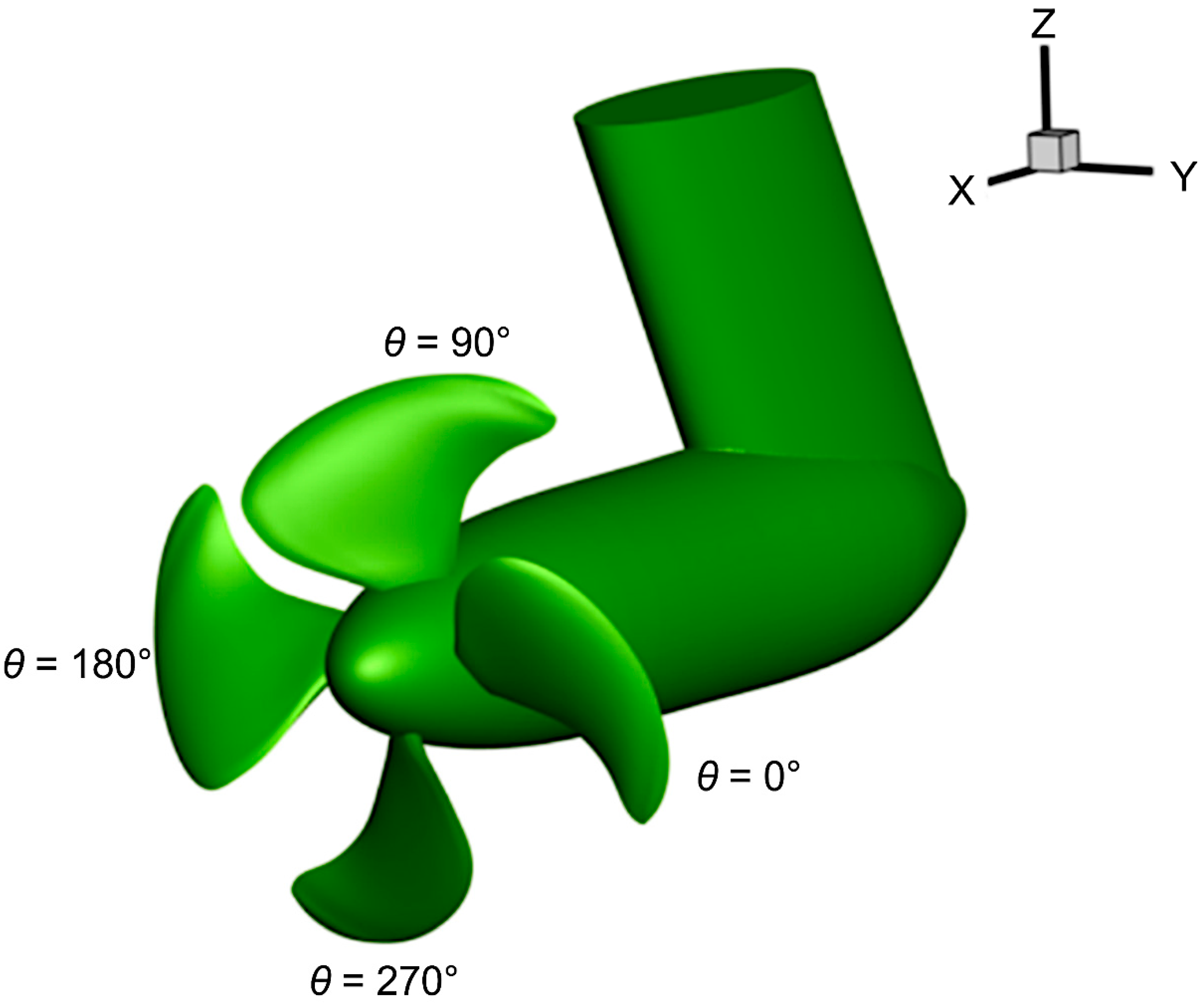
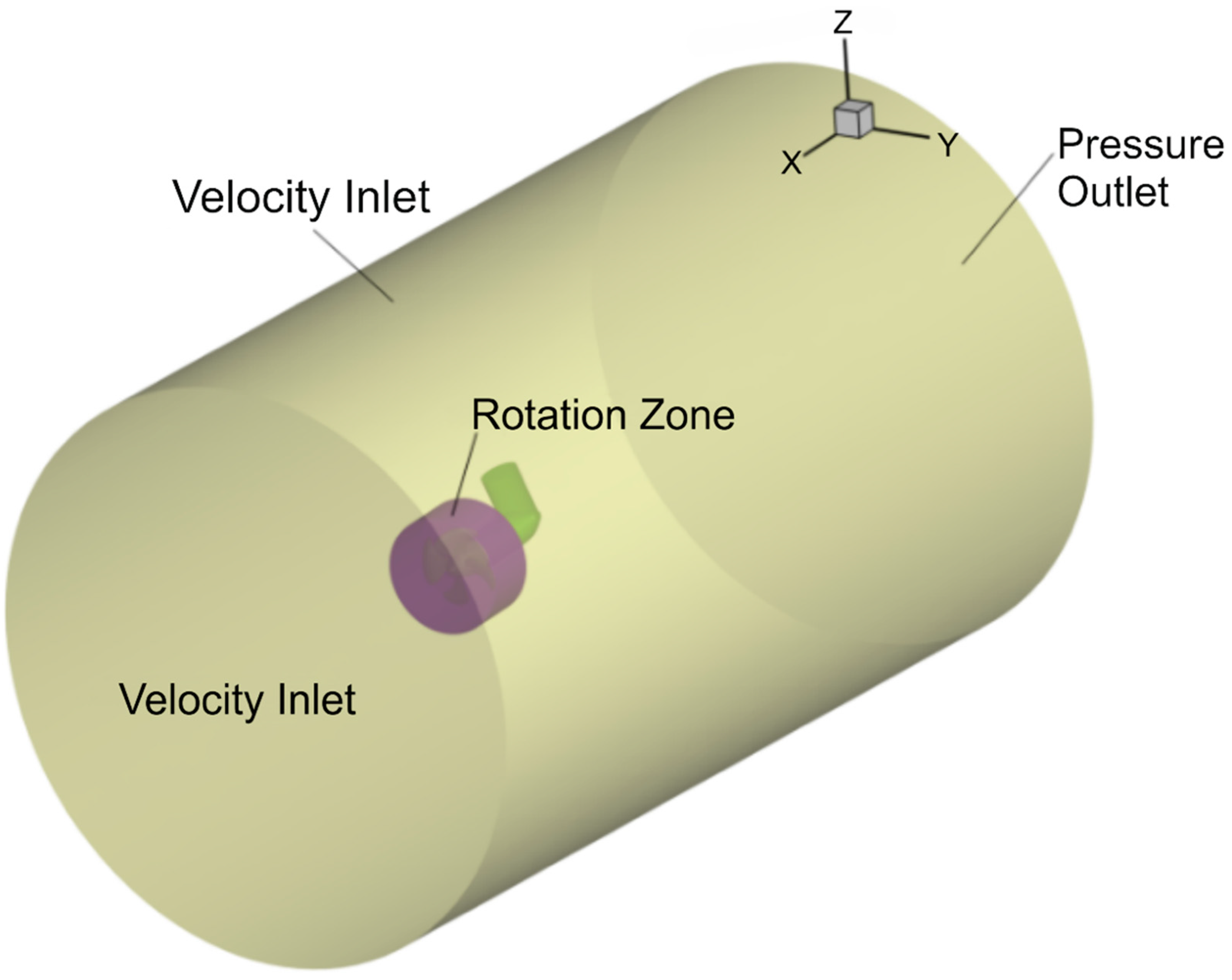
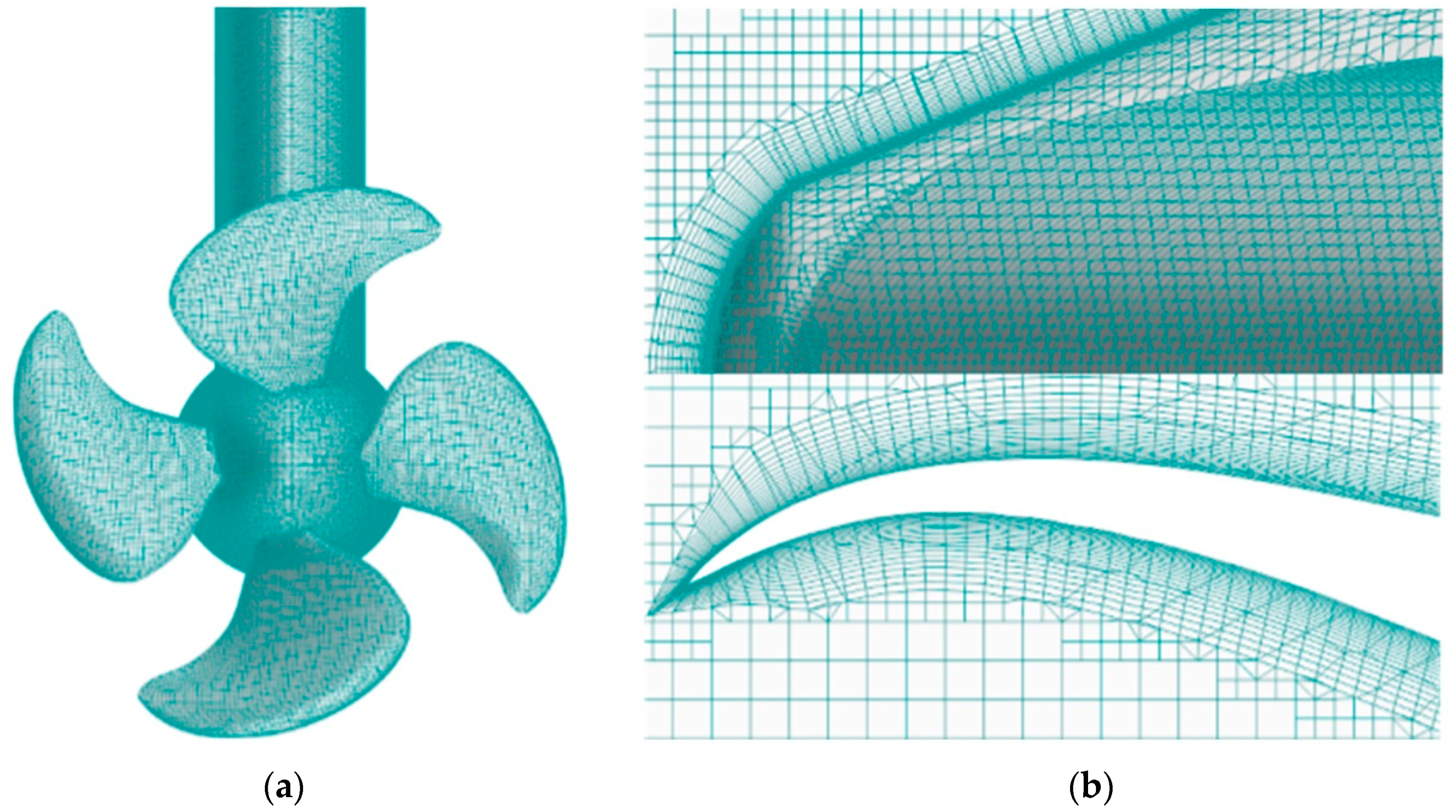
2.2. Geometric Model and Computational Grid

The podded propulsion model used in this study is obtained through a certain reduced scale ratio and local modification of an original CO1250 pod from the ABB company. Table 1 lists the relevant propeller parameters.
Figure 1 shows the inertial coordinate system used for the numerical calculations presented in this section. The x-axis points in the direction of the incoming flow and coincides with the rotation axis of the propeller. The z-axis points in the vertical upward direction, and the y-axis is determined according to the right-hand rule. Generally, oblique incoming flow can be simulated by adjusting the angle of the propeller model or changing the velocity component of the incoming flow. This study uses the latter approach because the amount of effort is reduced by establishing only one calculation model for both calculations: no oblique flow angle condition and with oblique flow angle condition. Figure 2 shows the selected computational domain.
The computational domain of the model is a cylinder. The diameter of the cylinder is 7.5 times that of the diameter of the propeller; the distance between the propeller and the inlet is 5 times that of the diameter of the propeller, and the distance between the propeller and the outlet is 9 times that of the diameter of the propeller. The inlet and side of the boundary are set to Velocity Inlet; the outlet is set to Pressure Outlet. The interface between the outer and propeller domains is set to Wall (non-slip wall), and the other unspecified parts are set to a non-slip wall condition.
In this study, the overlap grid technique was used for the numerical simulation. When calculating the hydrodynamic performance of propellers, it is necessary to maintain the propeller at a certain rotational velocity within the flow area. This was implemented according to the following procedure. First, the sliding-grid method was used to encase the propeller in a small region having the same axis as the propeller. Next, an appropriate background field was established, and an interface between the border of the above small region and the background region was generated. The boundary condition for this interface was set to an overset mesh. Finally, the numerical information of an unsteady flow field on the two boundary surfaces of the interface was relayed while the small region containing the propeller rotated at the preset speed.
Details of the mesh distribution for the coarse, medium and fine discretization levels are listed in Table 2. M stands for million.
This propeller has a 35° incline; therefore, the structured grid partition is complex and the grid quality is low. A cutting grid is used to conduct grid partitioning in the computational domain; the cutting grid is robust and effective and has good applicability to complex geometric models [18,19]. Note that locations where the curvature is significant—such as the leading edge, trailing edge, and blade root—should be locally densified when generating the grid. Additionally, to better simulate the boundary layer, a 20-layer prism grid is generated on the unit surface of the pod. The value of the dimensionless distance y+ from the first layer to the wall surface is taken as 30, and the grid partition form is as shown in Figure 3. The value of the wall unit, y+, is the main criterion in order to properly model the turbulent boundary layer and obtain the correct pressure distribution on the propeller blade surfaces. To directly resolve the viscous sub layer, in which the value of the wall unit, y+, requires quite the number of grids in sympathy with increasing the calculation time. Therefore, we implemented a wall function based on the blended wall law to gain the significant savings in terms of near-wall mesh resolution.
Table 3 presents the computed results for the thrust coefficient and torque coefficient for the three groups when the advance ratio J = 0.7. It can be observed from the table that both K T and 10 K Q exhibit a relatively low sensitivity to grid density.

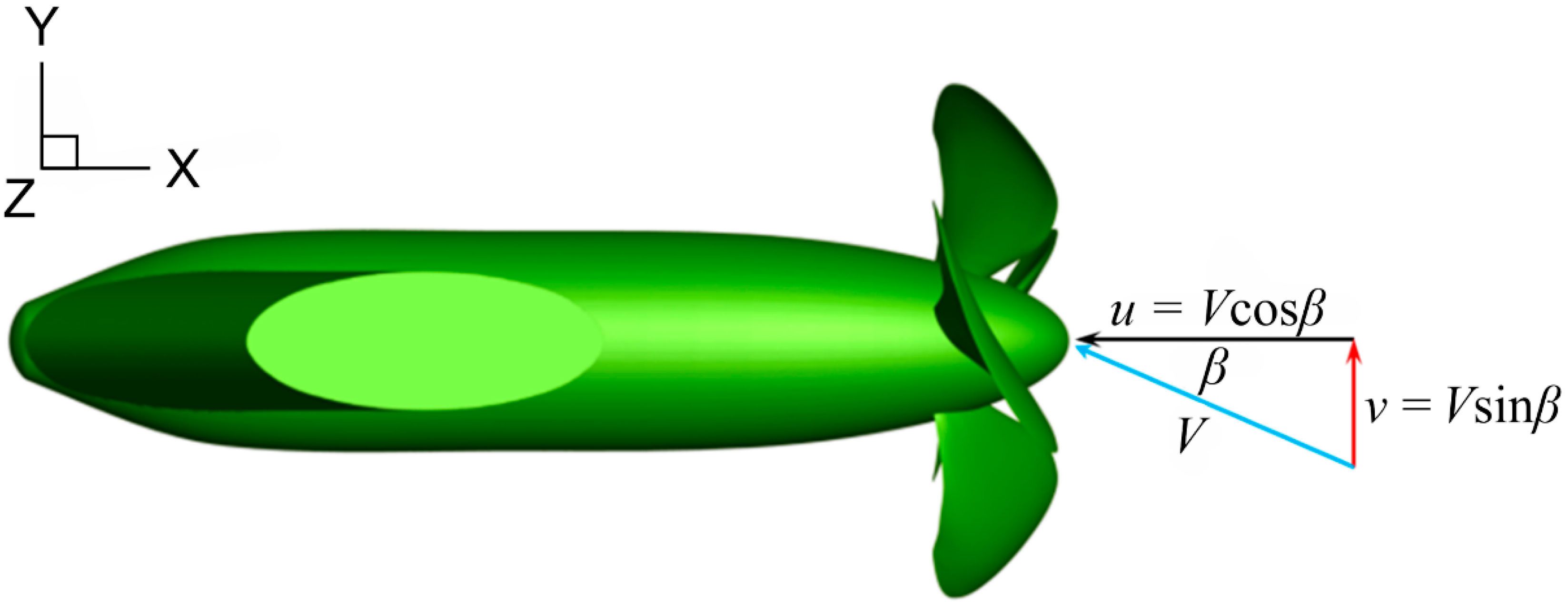
2.3. Parameter Setting and Operating Conditions

Figure 4 shows a schematic diagram of the incoming flow at the inlet. The oblique flow angle of the y-axis velocity component pointing in the y-axis positive direction is the negative oblique flow angle. In this study, calculations and experimental tests were performed for two advance coefficients of podded propulsion, J = 0.4 and 0.8, and six rudder angles for oblique navigation, ±5°, ±10°, ±15°, ±30°, ±45°, and ±60°. Table 4 lists the specific working conditions for the six calculations. Propeller rotation is achieved through sliding grid technology; coupling of pressure and velocity is solved using the SIMPLEC algorithm [20]; rotation and static zones are connected by the interface boundary; and flow field information is transferred through interface interpolation. The propeller hydrodynamic performance for different advance coefficients is obtained by changing the velocity of the incoming flow. The time step of the numerical calculation is 2.7778 × 10⁻⁴ s; this corresponds to the time required by the propeller to rotate by 1°.
K T P i and K Q P i are the thrust and torque coefficients of the propeller, respectively; η P is the open-water propeller efficiency; K T U i and K Q U i are the thrust and steering torque coefficients of the podded propulsion unit, respectively; and η U is the open-water propeller efficiency of the pod unit. These parameters are defined as follows:
K T P i = T P i ρ N 2 D 4 ;   K Q P i = Q P i ρ N 2 D 5 ;   η P = K T P i K Q P i · J 2 π ,
K T U i = T U i ρ N 2 D 4 ;   K Q U i = M z ρ N 2 D 5 ;   η U = K T U i K Q U i · J 2 π ,
where i = x, y, and z are the three directions of the inertial coordinate system; T P i and Q P i are the thrust and torque of the propeller, respectively; T U i is the thrust of the pod unit; M z is the steering torque of the pod unit; N is the rotation speed of the propeller; and D is the diameter of the propeller.

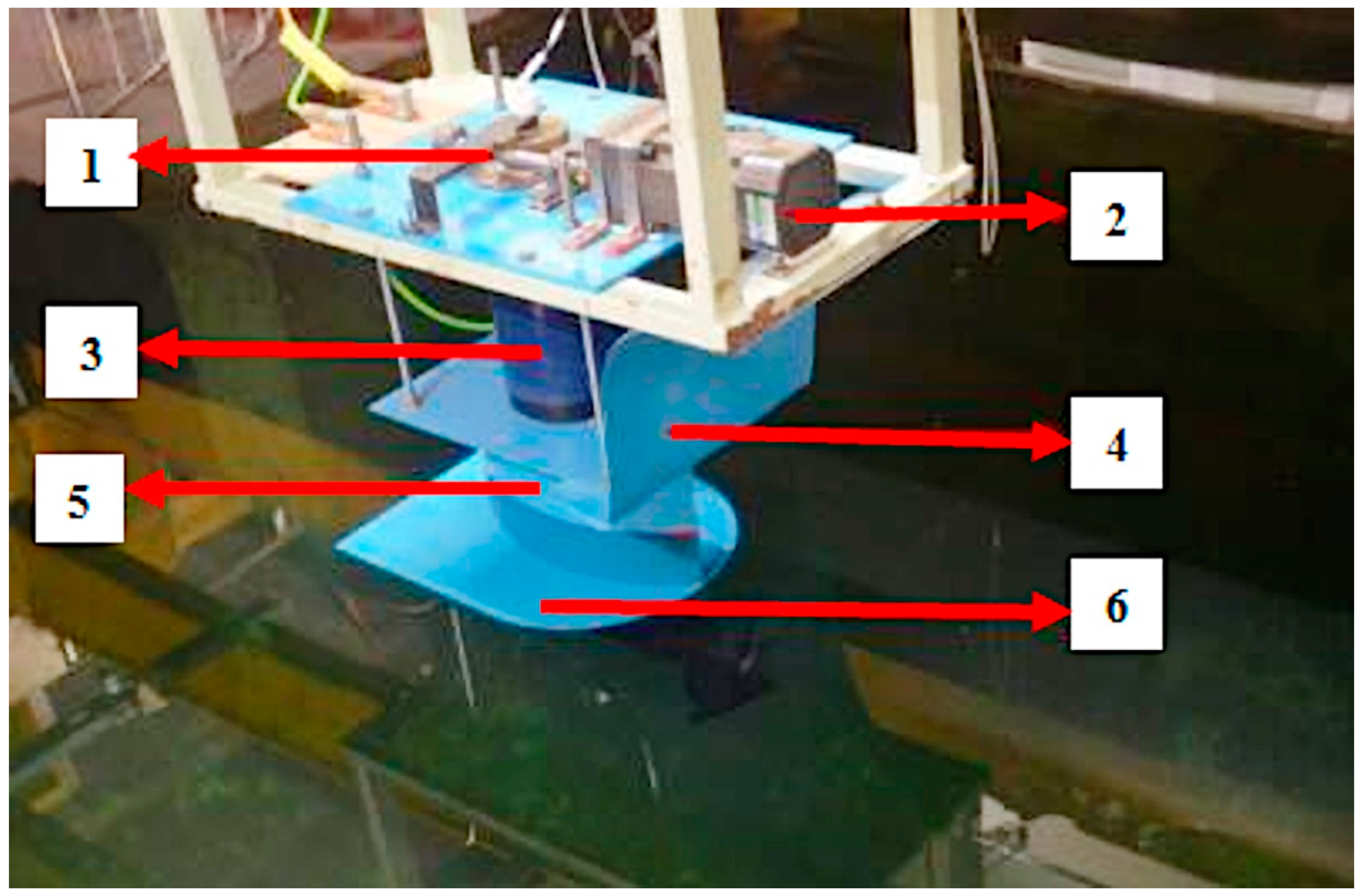
2.4. Model Experimental Test

The model experimental test was performed in the towing tank. A set of L-type podded propulsion devices was independently developed, and a series of experimental tests were conducted to evaluate the hydrodynamic performances of the podded propulsor. The propeller thrust, torque, and overall thrust of the podded propulsor unit were measured in the experiment under the condition of moving straight forward. The performance of the propeller and podded unit were compared under an oblique flow angle for two different advance coefficients of the L-type podded propulsor. The working conditions for the model test were the same as those in the numerical simulation.
Figure 5 shows the L-type podded propulsor testing system and its components: 1—Dial; 2—Steering motor; 3—Force sensor; 4—Billboard; 5—Deflector; 6—Water seal plate.
A towing tank and podded propulsor dynamometer developed by the authors were used for the experiment, which was conducted in two parts: The first part determined the forces, and the second part evaluated the flow field characteristics. The entire test apparatus was fixed to a trailer, and with the exception of the platform, all components could rotate 360° in the horizontal plane to satisfy the requirements of different operating conditions. The propeller rotation speed was fixed, and the experiment was conducted by manipulating the forward speed of the trailer. The draft depth of the propeller shaft was maintained at 0.4 m > 1.5D, as suggested by the ITTC.

3. Results and Analysis

The calculation results within the range J = 0.5–1.0 are compared with the experimental results obtained in the towing tank, as shown in Table 5. The calculation results are generally consistent with the experimental results, indicating that the proposed computing method for predicting the hydrodynamic performance of L-type podded propulsion is reliable.

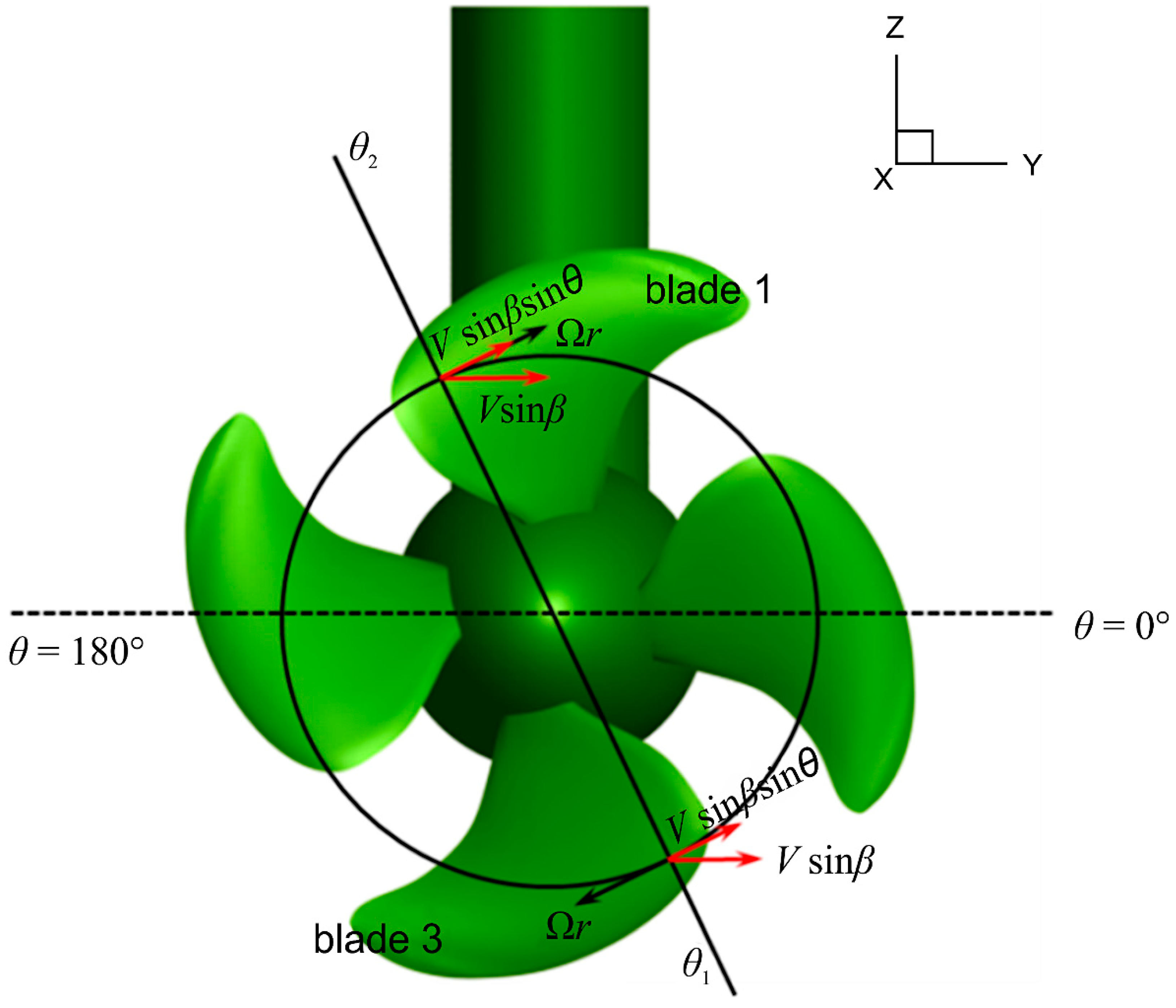
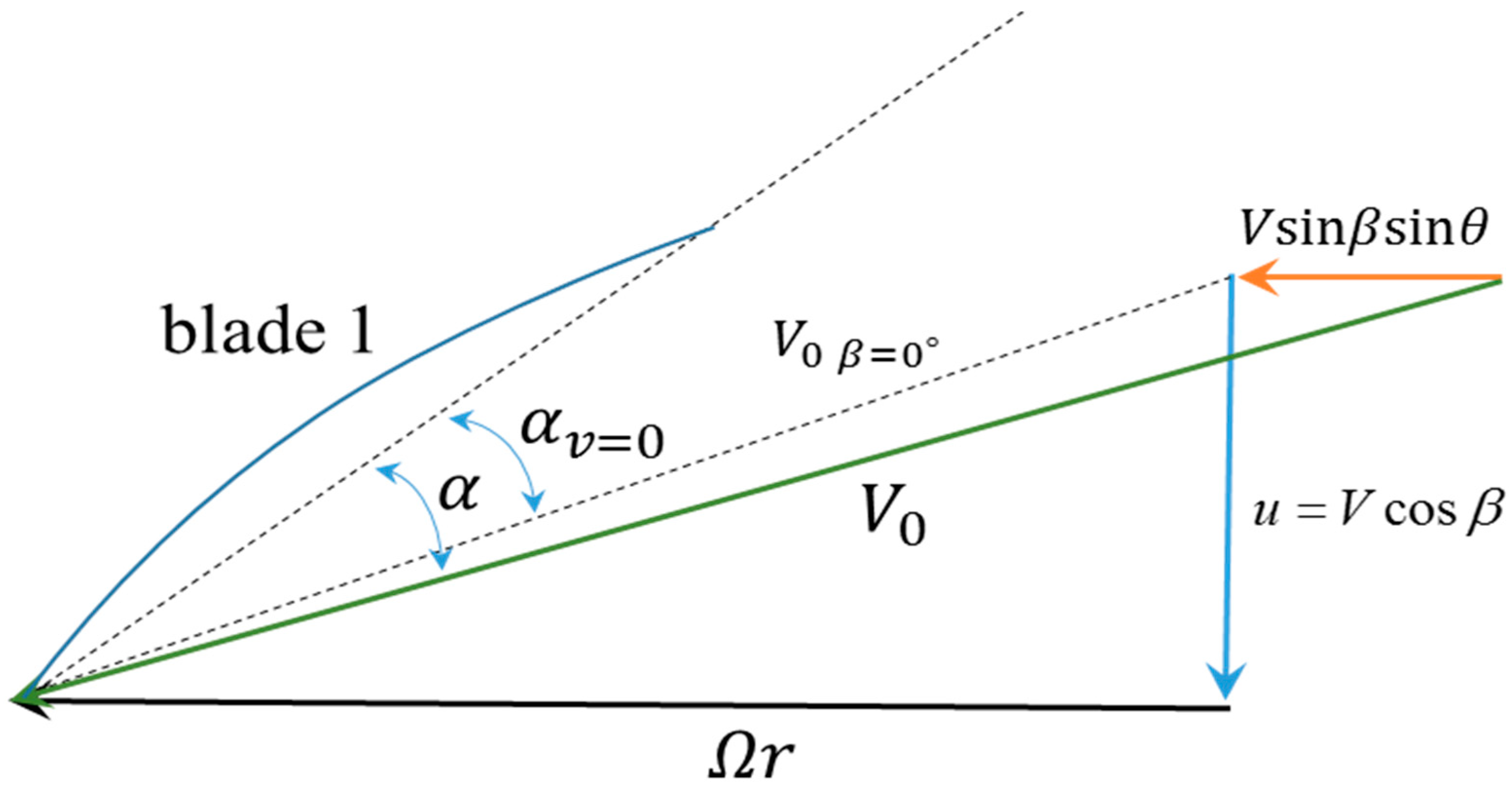
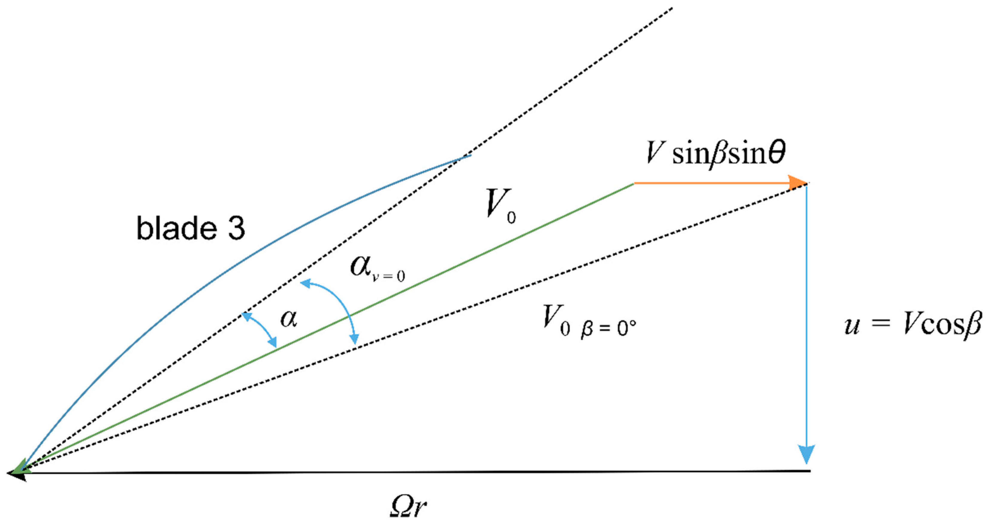
3.1. Calculation Results of Single Blade

Figure 6 shows the hydrodynamic force analysis of the profiles of blades 1 and 3 by taking the negative oblique flow angle as an example (y-axis velocity component points to the positive direction of the y-axis) to analyze the stress condition of a single blade during rotation more clearly.
The circumferential position of the blade for direct horizontal incoming flow is defined as θ = 180 ° , and it increases successively counterclockwise. The circumferential position of the blade for θ = 0 ° is as shown in Figure 6. The incoming flow of the blade section mainly contains an axial velocity component and a circumferential velocity component defined as follows:
{ u a x i a l = u = V cos β ν t a n g e n t i a l = Ω r + V sin β sin θ ,
where u is the oblique flow velocity; Ω , the velocity of the rotation angle of the propeller; β , the oblique flow angle; θ , the circumferential position of the blade; u a x i a l , the axial velocity component; and ν t a n g e n t i a l , the circumferential velocity component. Irrespective of the induced velocity of the propeller, the axial incoming flow u a x i a l is constant, that is, the axial component velocity u a x i a l is homogeneously symmetrical in the upper, lower, left, and right sides of the disk area of the propeller; this has the same effect on thrust and torque in all quadrants. By contrast, the circumferential velocity is not symmetric; therefore, the propeller generates an unsteady force. The rotation circumferential velocity of the blade Ω r is fixed for the specified radius position, whereas V sin θ cos θ relative to the circumferential position angle θ changes constantly during one rotation, leading to a constant change in the attack angle of the back profile:
α = Θ arc tan ( u a x i a l ν t a n g e n t i a l ) = Θ arc tan ( V cos β Ω r + V sin β sin θ ) ,
Θ is the pitch angle of the blade section; Equation (6) shows that the attack angle of the blade section and thrust generated by the blades increase with the axial velocity component.
Figure 7 and Figure 8 show the attack angle of the blade section with pure axial flow ( β = 0°). The attack angle of the blade section is respectively larger and smaller than that in pure axial flow for blades 1 and 3. Additionally, the analysis of the expression of the circumferential velocity component shows that the circumferential velocity varies sinusoidally; it has a maximum value at θ = 90 ° and a minimum value at θ = 270 ° . Equation (6) indicates that the attack angle of the blade section has a maximum value at θ = 90 ° and a minimum value at θ = 270 ° . The analysis results indicate that the blade thrust and torque reach their maximum at θ = 90 ° and their minimum at θ = 270 ° .
V 0   β = 0 is the inflow velocity when the oblique flow angle is zero, that is, the inflow velocity when the pure axial flow angle is zero, and its numerical value is equal to the inflow velocity value in Table 2. V 0 is the inflow velocity, and it is the same as V 0   β = 0 when the oblique flow angle is zero.
Figure 9 shows the thrust and torque of a single blade during one rotation when the oblique flow angle is 10 ° . The figure shows that the thrust and torque reach their maximum at θ = 90 ° and their minimum at θ = 270 ° , indicating the consistency between the calculation and analysis results. The peak value of blade force and moment should appear at 90 and 270 positions in the inclined flow. The deviation between the peak position in Figure 9 and the theoretical value should be caused by the interference of the propeller, cabin and bracket. The interaction between the propeller and pod not only cause the fluctuation of the propulsor performance, but also influence the downstream flow field and pressure distribution on the pod.

3.2. Experimental Results of Propeller

The asymmetry of the incoming flow in the propeller disk area may cause a change in the propeller force and moment under oblique flow and direct navigation states. This is a key problem in the study of propeller hydrodynamic performance under an oblique flow.
Figure 10 shows the relationships of propeller thrust and torque with oblique flow angle. For J = 0.4 and 0.8, the trend of change in propeller load with the oblique flow angle is generally consistent and shows a symmetrical distribution when the oblique flow angle is 0°. The thrust and torque of the propeller increase with the oblique flow angle. For J = 0.8, the thrust and torque with an oblique flow angle of 60° increase by 167% and 106%, respectively, compared to those with an oblique flow angle of 5°. By contrast, for J = 0.4, the thrust and torque with the same angle increase by only 35% and 30%, respectively, indicating that they are more sensitive to changes in the oblique flow angle under a high advance coefficient. The propeller thrust does not change obviously when the oblique navigation angle is small ( β 15 ° ); when the oblique navigation angle is larger than 15°, the propeller thrust and torque become more sensitive to the oblique flow angle. This result is mainly due to the constant towing velocity of 0.96, 1.92 m/s over the whole flow angle range. This implies a variable axial velocity over the angle beta. Hence, the difference between J = 0.4 and 0.8 changes over the beta angle influenced by the axial velocity difference.
Figure 11 shows the propeller efficiency with changing oblique flow angle. The figure shows that the propeller efficiency follows a different trend under two different loads. The torque of the propeller relative to the viscous effect increases with the thrust of the propeller relative to the pressure effect when the load is varied from high to low. For a high advance coefficient, the speed of increase of the pressure effect is higher than that of the viscous effect, and therefore, the propeller efficiency shows an increasing trend with an increase in the oblique flow angle. However, for a low advance coefficient, the propeller efficiency curve shows minimal change.

3.3. Experimental Results of Pod

Figure 12a shows the relationship between the thrust coefficient of the pod and the angle of oblique navigation. When oblique flow angle β is smaller than 15°, the total thrust coefficient of the pod changes slightly with an increase in the oblique flow angle and is mostly positive when advance velocity is lower. The projection of the pod bracket increases gradually with the angle of oblique navigation. The resistance increase caused by water flow impacting the lateral face of the bracket further leads to a rapid increase in resistance of the whole pod. The thrust decreases fast and then converts into resistance, resulting in a rapid decrease in the thrust coefficient of the pod. When the oblique flow angle is larger than a certain value, the thrust coefficient curve shows negative values. When parallel to the angle of oblique navigation, the total thrust value reduces as the advance coefficient increases.
Figure 12b shows the relationship between the lateral force coefficient of the pod and the angle of oblique navigation. The lateral force coefficient of the pod shows that the lateral force gradually increases with the advance coefficient and the angle of the oblique navigation (positive and negative features of the curve only indicate different steering directions). When the angle of oblique navigation is small ( β 15 ° ), the change in lateral force is not obvious. When the angle of oblique navigation is larger than 15°, the overall lateral force under different advance coefficients becomes apparent, but its velocity rate of change reduces with an increase in the angle.
The plane steering torque of the pod has a corresponding relationship with its lateral force, as shown in Figure 12c. The trend of the two advance coefficients is also similar. In the direct navigation state, the steering torque is not zero due to the influence of the wake flow field on propeller rotation. When the rudder angle is between 0° and 5° right, the plane stress of the whole pod that takes the center of the bracket as the rotation axis is in equilibrium and the plane steering torque is zero. With a further increase in the rudder angle and advance coefficient, the plane steering torque of the pod increases constantly, but the rate of change gradually decreases.
It can be seen from the figure that the thrust coefficient of the pod first decreases and then increases when the yaw angle is about 10 degrees, that is, stall occurs at this moment. Therefore, in the design or actual navigation of the L-type pod propeller, it is necessary to find this angle through research. When turning left or right, the effect of propeller rotation on POD propeller performance should be taken into account. In actual navigation, the angle should be crossed as soon as possible.

4. Discussion

This section compares and analyzes the pressure distribution and wake characteristics of L-type podded propulsion under different oblique flow angles and advance coefficients.

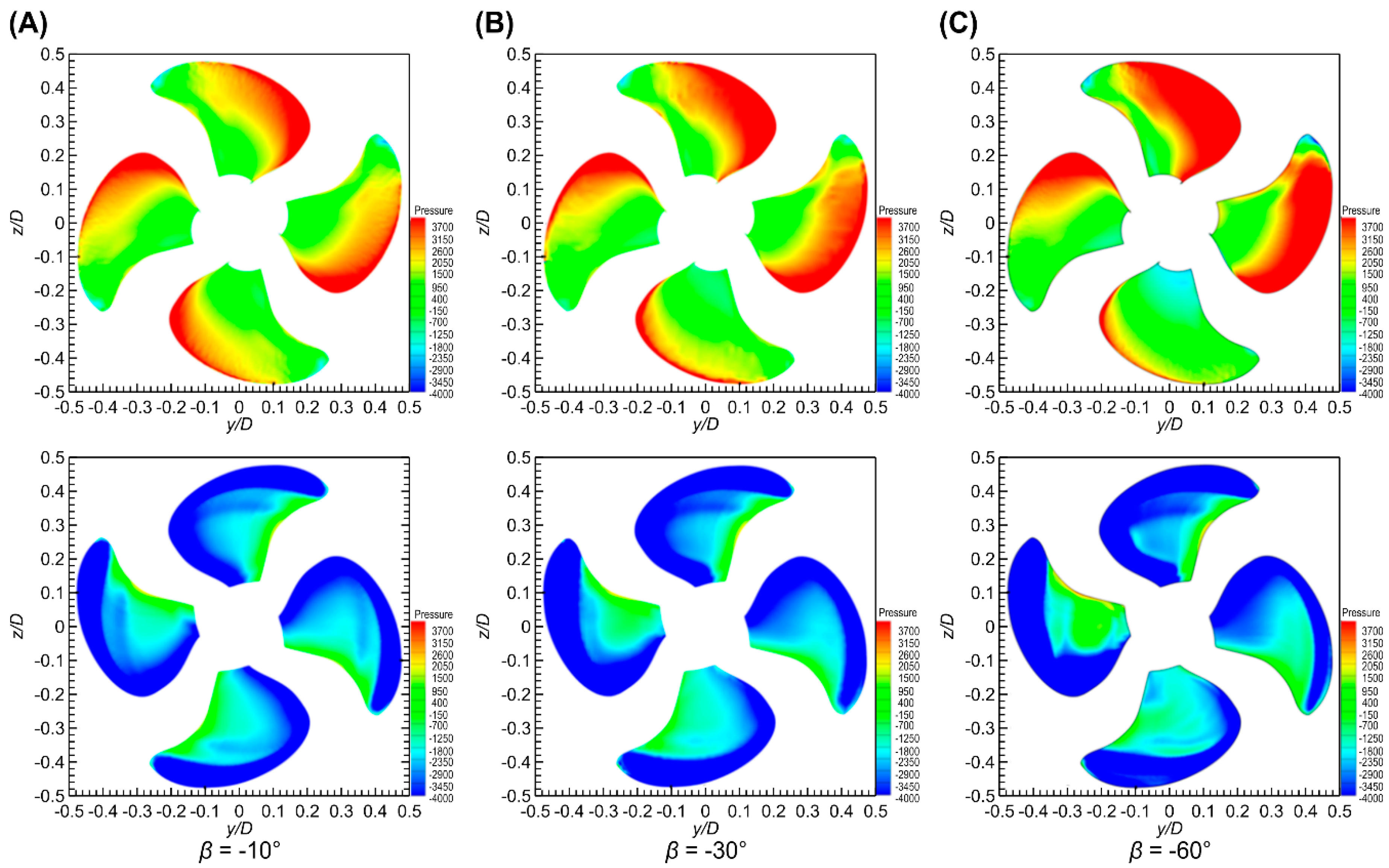
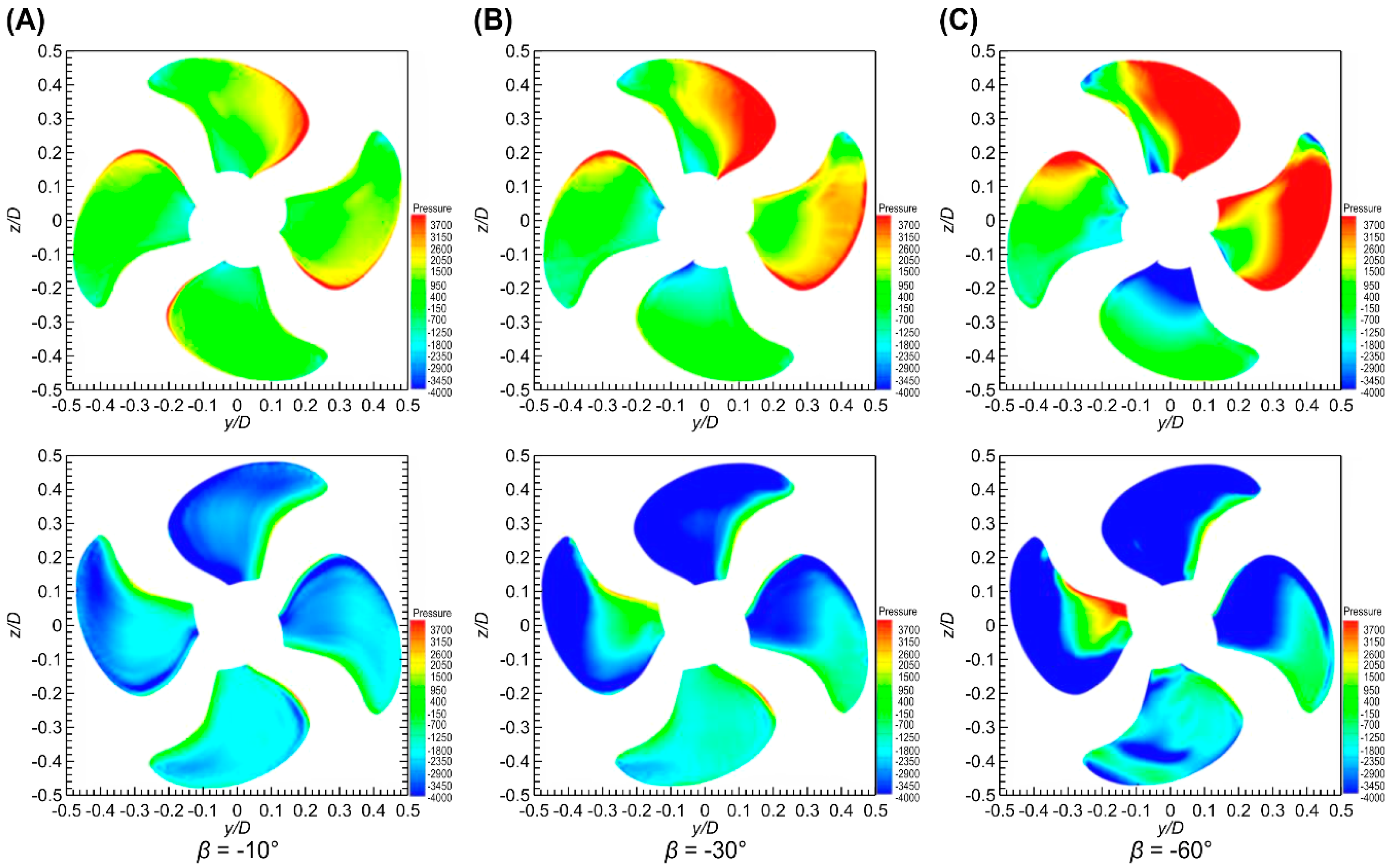
4.1. Calculation Results of Pressure Distribution

Figure 13 and Figure 14 show the propeller blade pressure distributions with different oblique flow angles of −10°, −30°, and −60° under advance coefficients of J = 0.4 and 0.8. Both the y-axis and z-axis adopt the propeller diameter D to become dimensionless. The figures show that the pressure on the blade surface is apparently higher than that on the back of the blade; this is why a propeller generates thrust. When the advance coefficient is low, the pressure difference between the blade surface and the back is high; however, with an increase in the advance coefficient, the pressure difference and propeller thrust decrease. The high-pressure area of the blade surface and low-pressure area of the blade back distribute at the side near the leading edge. The pressure from the leading edge to the blade tip clearly changes with a change in the oblique flow angle. There is a higher negative pressure zone at the leading edge of the blade back when the oblique flow angle increases; this further aggravates the production of vacuoles.
Additionally, the horizontal and vertical pressure distribution on the propeller blades has a different degree of asymmetry and nonuniformity. When the oblique flow angle is small, the pressure on the blade back and blade surface distributes evenly. When the oblique flow angle increases, the asymmetry of the pressure distribution becomes significant, and this asymmetry and nonuniformity enables the unsteady bearing force of the propeller to generate six pulsation components. This is the primary cause of the propeller producing an excitation force.
Equation (6) indicates that the blade load is the heaviest at θ = 90 ° and the pressure difference between the blade back and blade surface is the largest near θ = 90 ° in the corresponding pressure nephogram under negative oblique flow angles. In contrast, the blade load is the lightest at θ = 270 ° and the pressure difference between the blade back and blade surface is the smallest near θ = 270 ° .
The pressure distribution law can be obtained by summarizing the pressure distribution on the propeller blades, as shown in Figure 15. When the oblique flow angle is negative and the blade runs through the first and the fourth quadrants, its load is heavier than when running through the second and third quadrants. The load increases from θ = 270 ° to θ = 90 ° counterclockwise and reduces from θ = 90 ° to θ = 270 ° counterclockwise. When the oblique flow angle is positive, the characteristics are the opposite. When the blade runs through the second and third quadrants, its load is heavier than when running through the first and the fourth quadrants. The load reduces from θ = 270 ° to θ = 90 ° counterclockwise and increases from θ = 90 ° to θ = 270 ° counterclockwise.

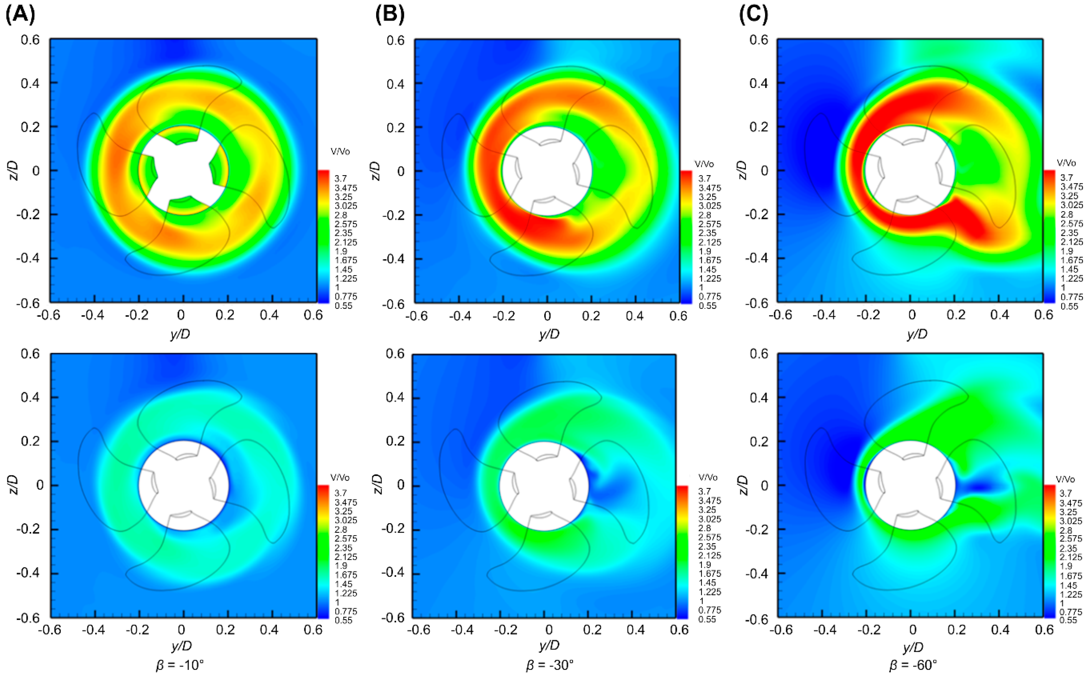
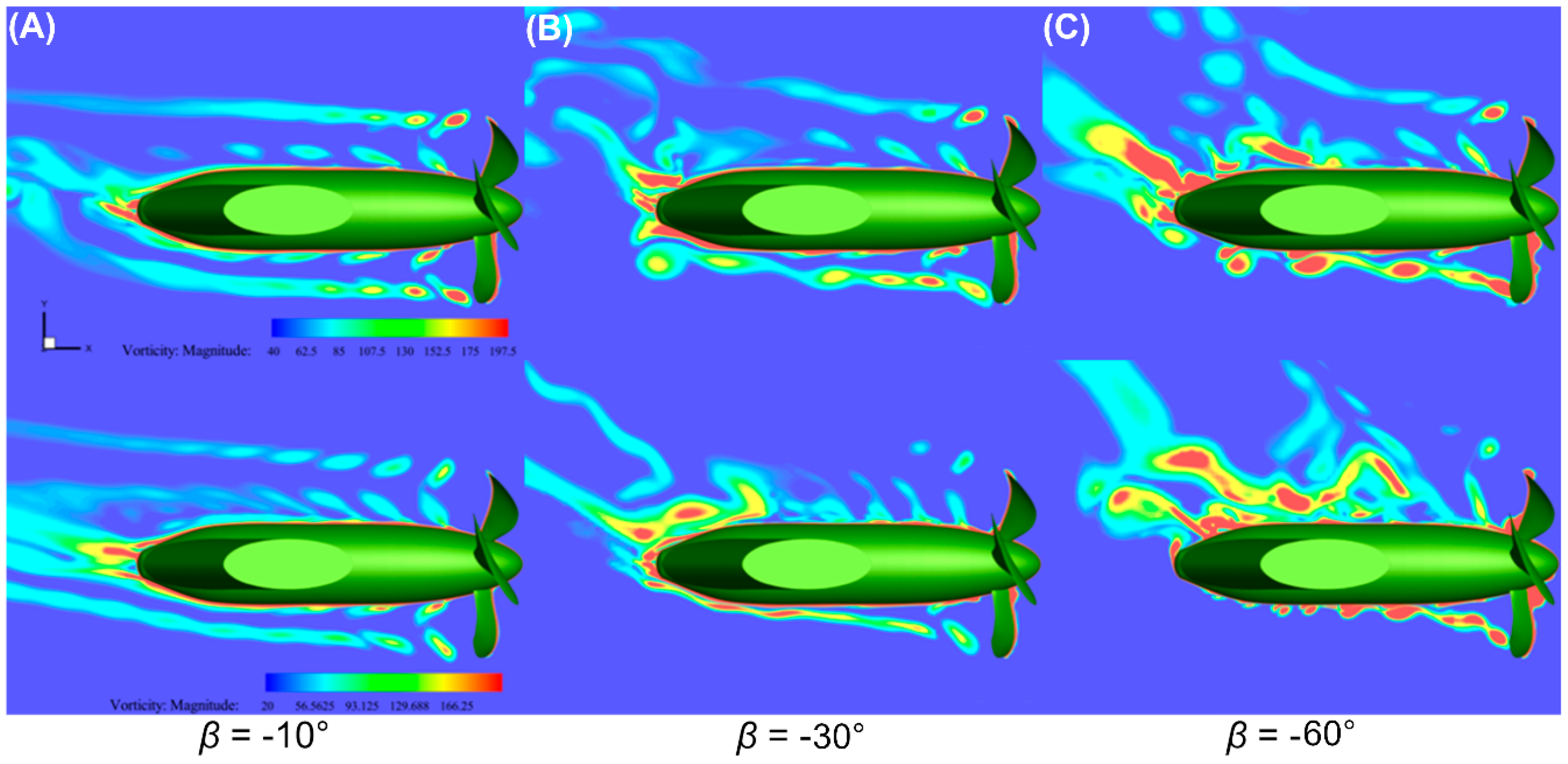
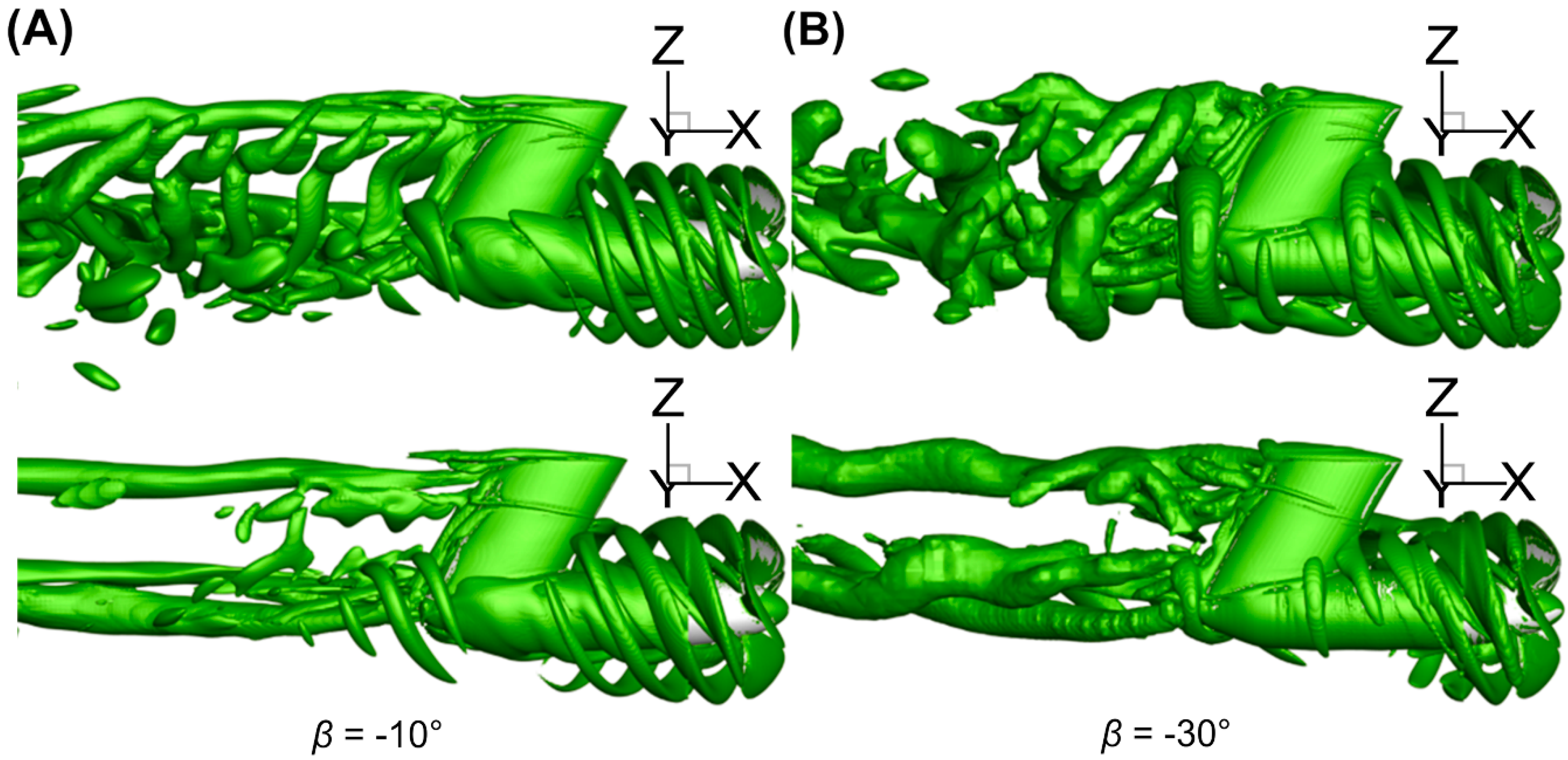
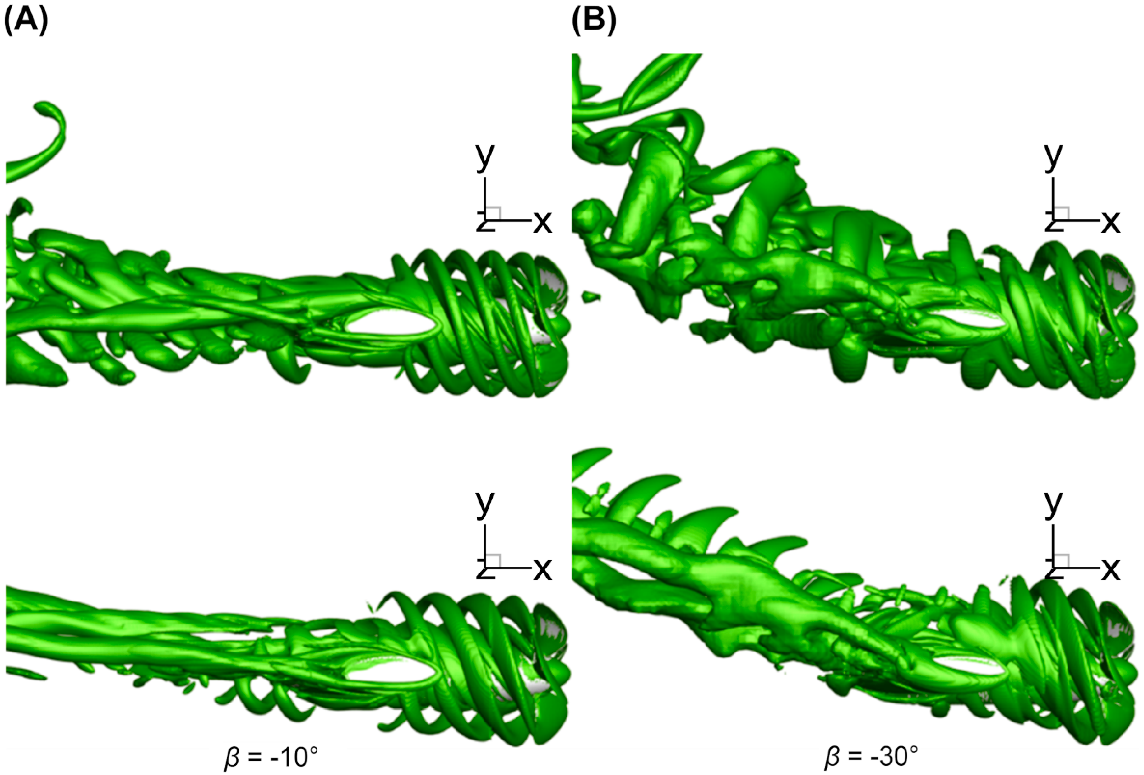
4.2. Calculation Results of Wake Flow Field

The successful application of the CFD method for the numerical simulation of a ship’s hydrodynamic performance enables extracting necessary flow field details from numerical results, except for the model test method. The analysis of the wake flow field of podded propulsion under oblique navigation is presented below.
Figure 16 shows the velocity distribution nephogram with the blade at x = −0.163 m under two advance coefficients when the oblique flow angle is negative. The velocity magnitude in this figure adopts propeller advance velocity V to become dimensionless. The velocity field after the blade shows different degrees of asymmetry and nonuniformity: Under a low advance coefficient and negative oblique flow angle, a high-velocity area surrounding the cabin appears in the negative semi-axis of the y-axis, and the range of the high-velocity area and velocity amplitude expands with an increase in the oblique flow angle. However, the high-velocity area in the negative semi-axis of the y-axis disappears with a high advance coefficient and a certain range of low-velocity area appears in the positive semi-axis of the y-axis. The distribution of the high- and low-velocity areas is closely related to the inflow of the propeller caused by the lateral velocity component of the incoming flow.
Figure 17 shows the vorticity distribution nephogram under two advance coefficients when the oblique flow angle is negative. It indicates that when the oblique flow angle is negative, the flowing energy is higher on the side of the negative semi-axis of the y-axis. When the oblique flow angle increases, the flowing energy also clearly increases. In addition, when the oblique flow angle is small, the vortex structure profile after the blade is relatively clear. When the oblique flow angle increases, the vortex systematic distribution after the blade becomes very disordered, because when the oblique flow angle is large, there is a strong interference effect between the venting vortexes and the cabin after the blades, resulting in a disorderly venting vortex system after the blade. Under a negative oblique angle, the tip vortexes after the blade have a trend skewing to the positive direction of the y-axis and the skew aggravates with an increase in the oblique flow angle caused by the lateral velocity components of different incoming flows.
The Q-crit β = 60 ° erion proposed by Hunt et al. [21] can be used to identify the vortex structure. When Q > 0, there are vortexes; otherwise, there are none. The size of Q is independent of the coordinate system selected. Figure 18 shows a side view of the vortex structure of podded propulsion under a negative oblique flow angle. It clearly shows the structures of the tip vortexes of the blades and trailing vortexes of the cabin and bracket, which demonstrates that the proposed grid partition and numerical calculation method can accurately capture the vortex structure when the pod is in an oblique navigation state. From the comparison of the vortex structure of the pod for advance coefficients of J = 0.4 and 0.8, it can be seen that when the advance coefficient is large, the screw pitch between the tip vortexes of the propeller is relatively large. When the advance coefficient is small, a larger number of vortexes fall off from the surface of the blades and cabin, leading to fierce turbulence pulsation. The comparison of the vortex structure of different oblique flow angles also shows that when the angle increases, a larger number of vortexes are emitted from the surface of the cabin and blades. Additionally, it is obvious that the bracket has a rectification effect because the rotation of water flow weakens when flowing through the bracket, whereas water that does not flow through the bracket emerges along the cabin vertically.
Figure 19 shows a top view of the vortex structure of podded propulsion under a negative oblique flow angle. The figure shows that the trailing vortex of podded propulsion has a trend skewing in the positive direction of the y-axis at different oblique flow angles. The trailing vortex has a trend skewing in the positive direction of the y-axis at a negative oblique flow angle, and the skew aggravates with an increase in the oblique flow angle. Furthermore, this skew is more severe after separating from the pod. As the flow runs downstream, the interference of podded propulsion on the flow field weakens gradually and the flowing direction is basically the same as the upstream incoming flow.
The water seal plate will greatly reduce the eddy current at the top of the pod struts and it has a good blocking effect on the top of the pod struts. In realistic conditions, the tip of the podded propulsor is not attached to the ship hull, and there will probably be a gap. For this reason, a tip vortex probably will exist, but with a different intensity; hence, interactions with the closer tip vortices will be different.

5. Conclusions

In this study, on the basis of the RANS method and a model experimental test, the unsteady hydrodynamic performance of L-type podded propulsion for 12 oblique flow angles (±5°, ±10°, ±15°, ±30°, ±45°, and ±60°) and 2 advance coefficients ( J = 0.4 and 0.8) was compared and analyzed. The change in load of a single blade, propeller, and pod under different oblique flow angles and wake flow fields was analyzed in detail. The following conclusions can be drawn from this study:
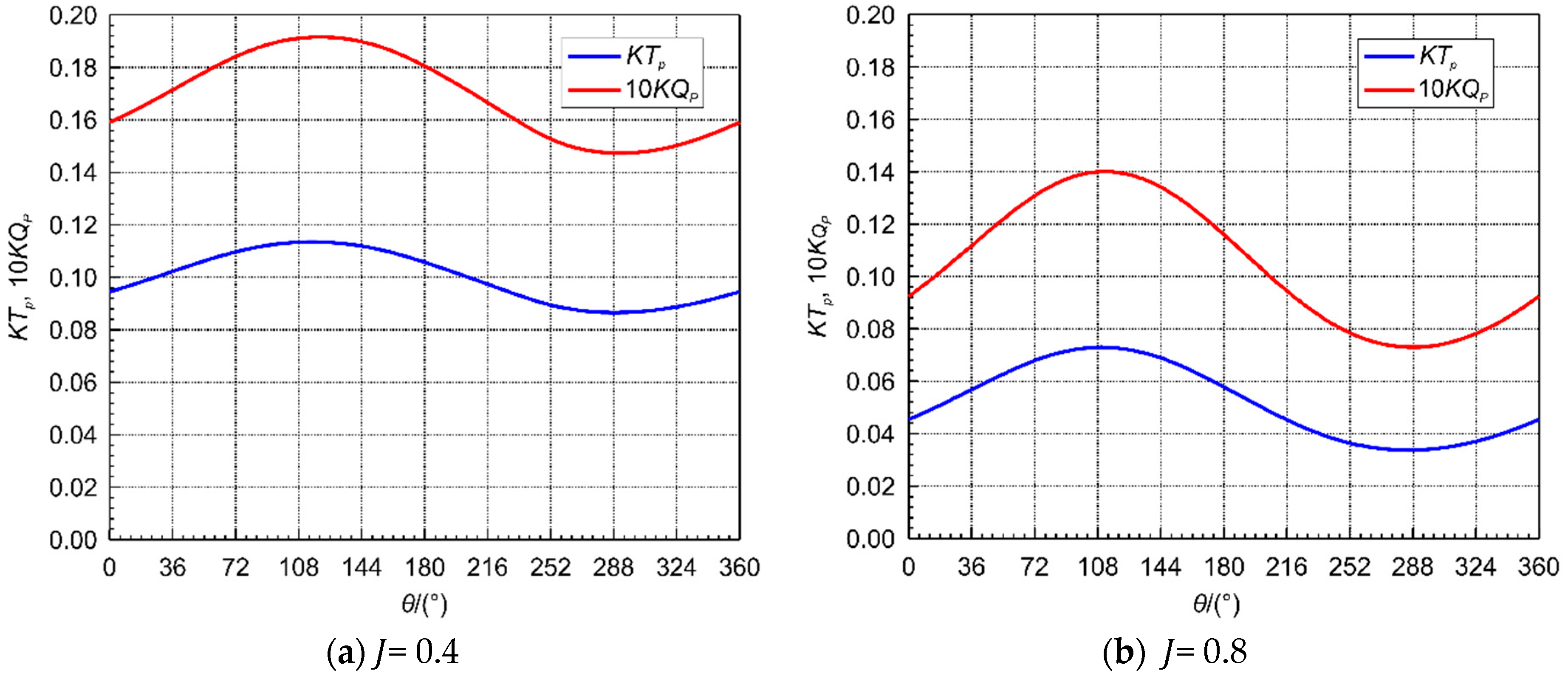
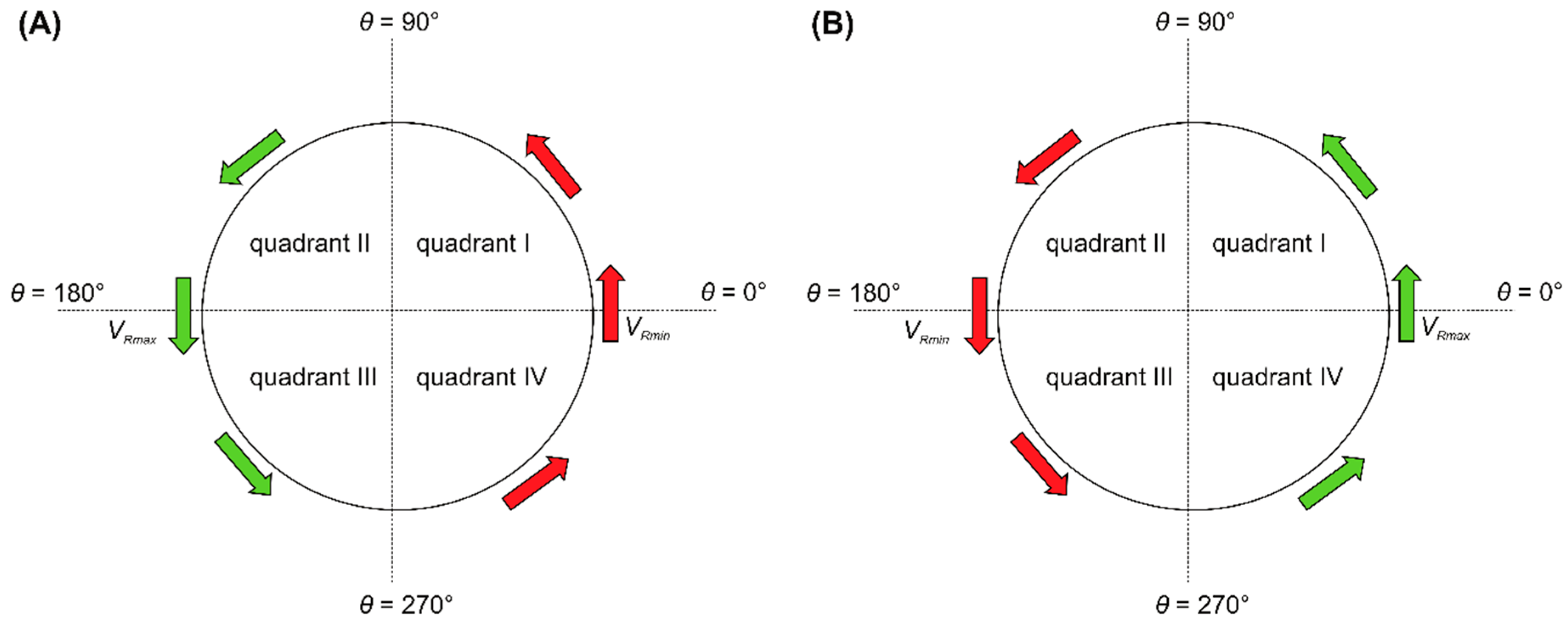
  • The change in circumferential velocity when the propeller rotates in an oblique flow leads to a constant change in the attack angle of the blade section. Under negative flow, the blade thrust and torque are the highest at θ = 90 ° and smallest at θ = 270 ° .
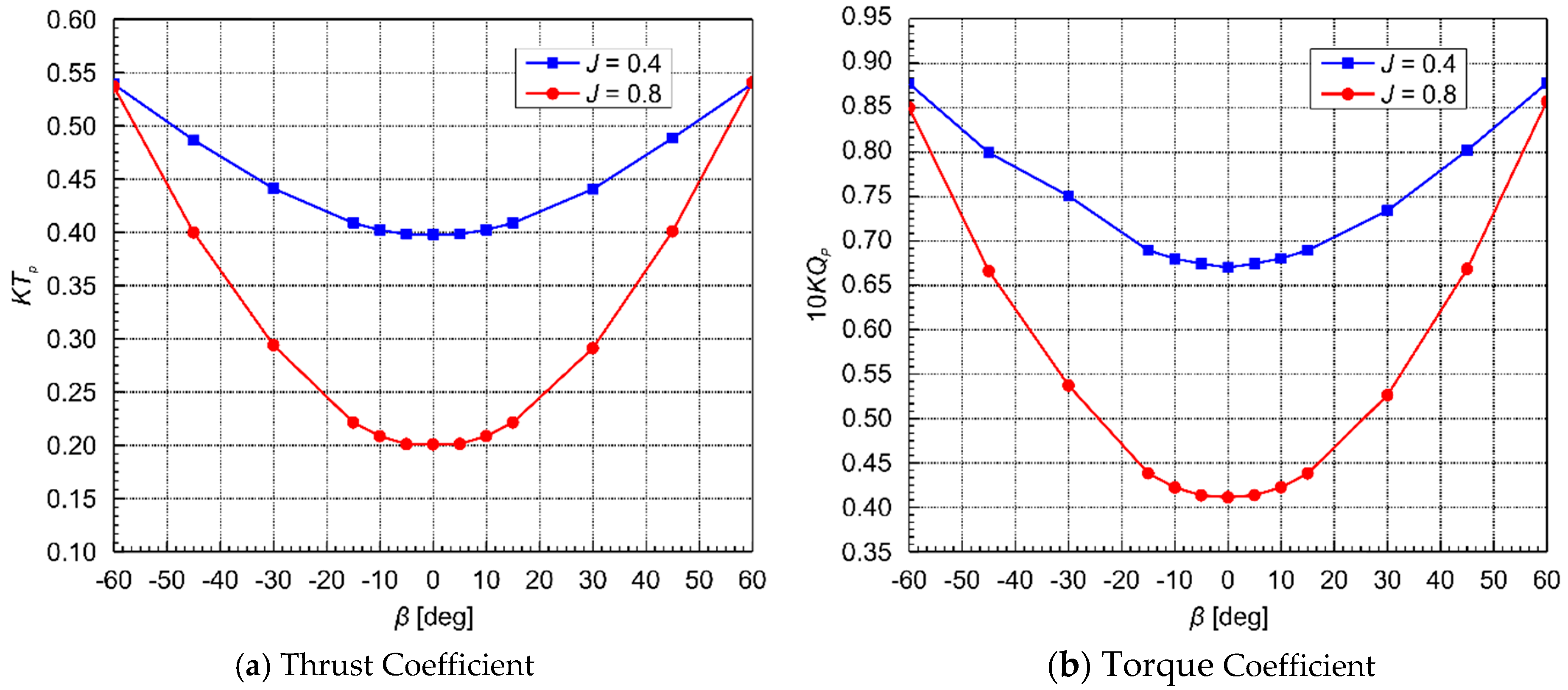
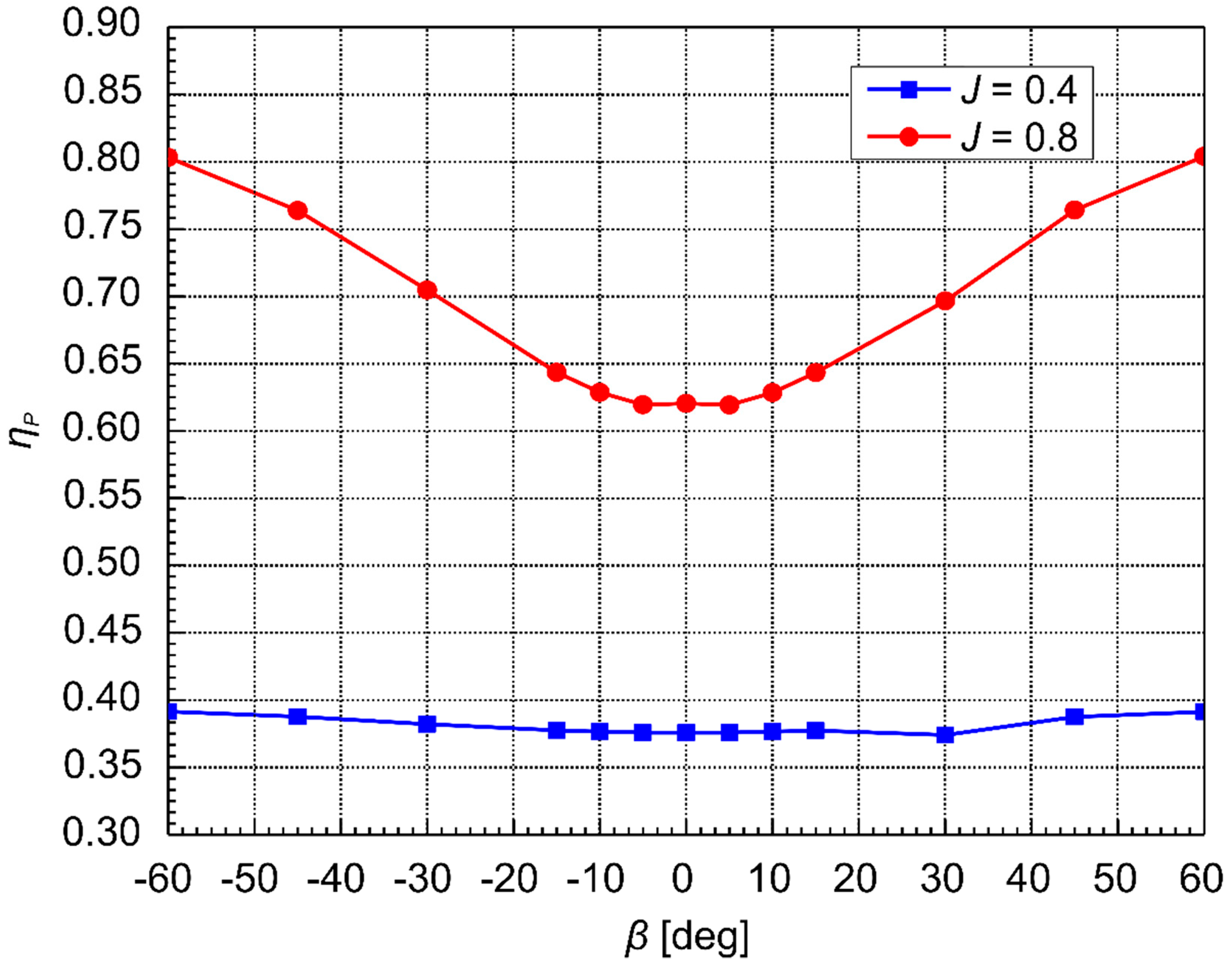
  • The load of the propeller under oblique flow will increase with the oblique flow angle. The increased resistance caused by water flow leads to a decrease in the podded propulsion thrust coefficient with an increase in the oblique flow angle. Under a high advance coefficient, the speed of increase of the pressure effect is higher than that of the viscous effect, and therefore, the propeller efficiency shows an increasing trend with the increase of the oblique flow angle. Under a low advance coefficient, the propeller efficiency curve changes gently.
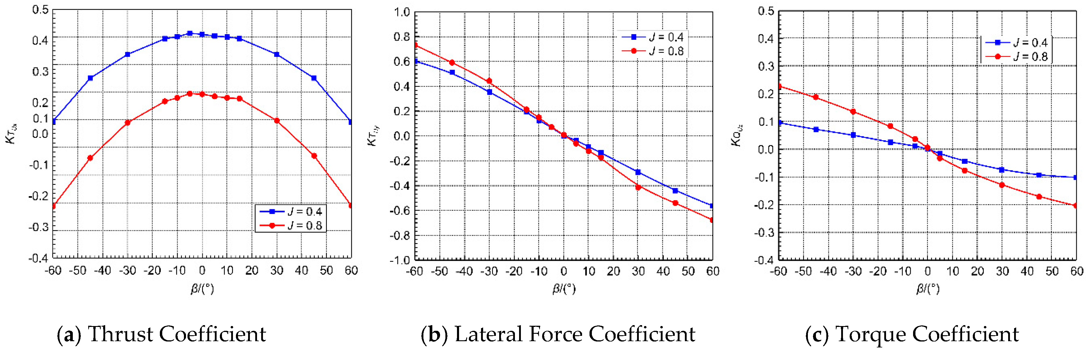
  • The nonuniformity of inflow results in varying degrees of asymmetry in the horizontal and vertical distributions of the propeller blade pressure, and this asymmetry is closely related to the size of the oblique flow angle and circumferential position of blades.
  • The velocity field after the blade shows different degrees of asymmetry and nonuniformity due to the lateral velocity component of the incoming flow. When the oblique flow angle was large, relatively strong interference effects between venting vortexes and the cabin after the blades were identified, leading to a disorderly venting vortex system after the blade.

Author Contributions

Conceptualization, W.W.; Writing—review and editing, D.Z.; Writing—original draft preparation, D.Z.; Methodology, C.G.; Formal analysis, Y.P.

Funding

The research was financially supported by the National Natural Science Foundation of China, Grant No. 51709060 and 51609030, Fundamental Research Funds for the Central Universities, Grant No. HEUCF180101 and HEUCF180104, and National High Technology Joint Research Program of China, Grant No. (2016) 548.

Acknowledgments

Many people have offered me valuable help in my thesis writing. I want to take this chance to thank my tutor. In the process of composing this paper, he gave me many academic and constructive advices and helped me to correct my paper. In addition, he also gave me the opportunity to do my teaching practice. Of course, I do need to thank my parents, because of their warm care I could grow up well.

Conflicts of Interest

The authors declare no conflict of interest. The funders had no role in the design of the study; in the collection, analyses, or interpretation of data; in the writing of the manuscript, or in the decision to publish the results.

References

  1. Shen, X.; Sun, Q.; Wei, Y.; Wu, Y.; Wang, H. Experimental investigation on hydrodynamic performance of podded propulsor under static azimuthing conditions. Shipbuild. Chin. 2016, 3, 9–18. (In Chinese) [Google Scholar]
  2. Zhao, C.; Yang, C.J. CFD simulation of propeller open-water performance considering induced velocity at the inlet of computational domain. Ocean Eng. 2014, 3, 72–77. [Google Scholar]
  3. Fu, H.P. Numerical study of methods for predicting integral hull and propeller and propeller-induced hull surface pressure fluctuations. J. Harbin Eng. Univ. 2009, 7, 728–734. (In Chinese) [Google Scholar]
  4. Chicherin, I.A.; Lobatchev, M.P.; Pustoshny, A.V.; Sanchez, C.A. On a propulsion prediction procedure for ships with podded propulsors using RANS-code analysis. In Proceedings of the 1st International Conference on Technological Advances in Podded Propulsion, Newcastle University, Newcastle, UK, 14–16 April 2004; pp. 223–236. [Google Scholar]
  5. Ohashi, K.; Hino, T. Numerical simulations of flows around a ship with podded propulsor. In Proceedings of the 1st International Conference on Technological Advances in Podded Propulsion, Newcastle University, Newcastle, UK, 14–16 April 2004; pp. 211–221. [Google Scholar]
  6. Liu, P.; Islam, M.; Veitch, B. Unsteady hydromechanics of a steering podded propeller unit. Ocean Eng. 2009, 36, 1003–1014. [Google Scholar] [CrossRef]
  7. Amini, H.; Sileo, L.; Steen, S. Numerical calculations of propeller shaft loads on azimuth propulsors in oblique inflow. J. Mar. Sci. Technol. 2012, 17, 403–421. [Google Scholar] [CrossRef]
  8. Guo, C.Y.; Ma, N.; Yang, C.J. Numerical simulation of a podded propulsor in viscous flow. J. Hydrodyn. Ser. B 2009, 21, 71–76. [Google Scholar] [CrossRef]
  9. Zhou, K.F.; Yan, T.; Guo, C.Y. CFD study of the hydrodynamic performances of L-type podded propulsor. Ship Eng. 2011, S2, 65–68. [Google Scholar]
  10. Xiong, Y.; Sheng, L.; Yang, Y. Hydrodynamics performance of podded propulsion at declination angles. J. Shanghai Jiaotong Univ. 2013, 6, 956–961. (In Chinese) [Google Scholar]
  11. The 23rd International Towing Tank Conference. Recommended Procedures. Propulsion Performance—Podded Propeller Tests and Extrapolation 7.5-02-03-01.3, Revision 00. 2002. Available online: https://ittc.info/media/1832/75-02-03-013.pdf (accessed on 20 February 2019).
  12. Reichel, M. Manoeuvring forces on azimuthing podded propulsor model. Pol. Marit. Res. 2007, 14, 3–8. [Google Scholar] [CrossRef]
  13. Islam, M.F.; Akinturk, A.; Veitch, B.; Liu, P. Performance characteristics of static and dynamic azimuthing podded propulsor. In Proceedings of the 1st International Symposium on Marine Propulsors, Trondheim, Norway, 22–24 June 2009; pp. 482–492. [Google Scholar]
  14. Islam, M.F.; Veitch, B.; Liu, P.F. Experimental Research on Marine Podded Propulsors. J. Nav. Archit. Mar. Eng. 2009, 4, 57–71. [Google Scholar] [CrossRef]
  15. Palm, M.; Jurgens, D.; Bendl, D. Boundary layer control of twin skeg hull form with reaction podded propulsion. In Proceedings of the 2nd International Symposium on Marine Propulsors, Hamburg, Germany, 15–17 June 2011. [Google Scholar]
  16. Wilcox, D.C. Turbulence Modeling for CFD; DCW Industries: La Canada, CA, USA, 1993; p. 460. [Google Scholar]
  17. Menter, F.R. Two-equation eddy-viscosity turbulence models for engineering applications. AIAA J. 2012, 32, 1598–1605. [Google Scholar] [CrossRef]
  18. Baek, D.G.; Yoon, H.S.; Jung, J.H.; Kim, K.S.; Paik, B.G. Effects of the advance ratio on the evolution of a propeller wake. Comput. Fluids 2015, 118, 32–43. [Google Scholar] [CrossRef]
  19. Meinke, M.; Schneiders, L.; Günther, C.; Schröder, W. A cut-cell method for sharp moving boundaries in Cartesian grids. Comput. Fluids 2013, 85, 135–142. [Google Scholar] [CrossRef]
  20. Weiss, J.M.; Smith, W.A. Preconditioning applied to variable and constant density flows. AIAA J. 1995, 33, 2050–2057. [Google Scholar] [CrossRef]
  21. Hunt, J.C.R.; Wray, A.A.; Moin, P. Eddies, Stream, and Convergence Zones in Turbulent Flows; Center for Turbulence Research Report CTR-S88; Stanford University: Palo Alto, CA, USA, November 1988; pp. 193–208. [Google Scholar]
Figure 1. Reference coordinate system.
Jmse 07 00051 g001
Figure 2. Computational domain of oblique flow.
Jmse 07 00051 g002
Figure 3. Computational grid of propeller. (a) Overall grid; (b) Boundary layer grid.
Jmse 07 00051 g003
Figure 4. Schematic diagram of oblique flow and incoming flow of podded propulsion.
Jmse 07 00051 g004
Figure 5. L-Type podded propulsor testing system.
Jmse 07 00051 g005
Figure 6. Hydrodynamic analysis of blade section in oblique flow (negative oblique flow angle).
Jmse 07 00051 g006
Figure 7. Velocity polygon of profile of blade 1.
Jmse 07 00051 g007
Figure 8. Velocity polygon of profile of blade 3.
Jmse 07 00051 g008
Figure 9. Pulsation curves of thrust coefficient and torque coefficient of single blade ( β = 10 ° ). (a) Pulsation curves at J = 0.4; (b) Pulsation curves at J = 0.8.
Jmse 07 00051 g009
Figure 10. Impact of oblique flow angle on propeller load. (a) Impact of oblique flow angle on thrust coefficient; (b) Impact of oblique flow angle on torque coefficient.
Jmse 07 00051 g010
Figure 11. Impact of oblique flow angle on propeller efficiency.
Jmse 07 00051 g011
Figure 12. Impact of oblique navigation angle on pod load. (a) Impact of oblique navigation angle on thrust coefficient; (b) Impact of oblique navigation angle on lateral force coefficient; (c) Impact of oblique navigation angle on steering torque coefficient.
Jmse 07 00051 g012
Figure 13. Pressure distribution of blade with negative oblique angle and J = 0.4 (top: blade surface; bottom: blade back). (A) Pressure distribution at β = 10 ° ; (B) Pressure distribution at β = 30 ° ; (C) Pressure distribution at β = 60 ° .
Jmse 07 00051 g013
Figure 14. Pressure distribution of blade with negative oblique angle and J = 0.8 (top: blade surface; bottom: blade back). (A) Pressure distribution at β = 10 ° ; (B) Pressure distribution at β = 30 ° ; (C) Pressure distribution at β = 60 ° .
Jmse 07 00051 g014
Figure 15. Blade pressure distribution law. (A) Negative oblique flow angle; (B) Positive oblique flow angle.
Jmse 07 00051 g015
Figure 16. Velocity distribution with blade at x = 0.163   m when oblique flow angle is negative (top: J = 0.4; bottom: J = 0.8). (A) Velocity distribution at β = 10 ° ; (B) Velocity distribution at β = 30 ° ; (C) Velocity distribution at β = 60 ° .
Jmse 07 00051 g016
Figure 17. Vortex nephogram after blade when oblique flow angle is negative (top: J = 0.4; bottom: J = 0.8). (A) Vortex nephogram at β = 10 ° ; (B) Vortex nephogram at β = 30 ° ; (C) Vortex nephogram at β = 60 ° .
Jmse 07 00051 g017
Figure 18. Side view of vortex structure after blade with a negative oblique angle when Q-criterion = 150 (top: J = 0.4; bottom: J = 0.8). (A) Vortex structure at β = 10 ° ; (B) Vortex structure at β = 30 ° .
Jmse 07 00051 g018
Figure 19. Top view of vortex structure after blade with a negative oblique angle when Q-criterion = 150 (top: J = 0.4; bottom: J = 0.8). (A) Vortex structure at β = 10 ° ; (B) Vortex structure at β = 30 ° .
Jmse 07 00051 g019
Table 1. Essential parameters of L-type podded propulsion.
Parameter (Units)Value
Long axis distance of cross section of inclined bracket (m)0.16
Short axis distance of cross section of inclined bracket (m)0.062
Height between upper surface of inclined bracket and y-axis (m)0.19
Inclined angle of bracket (°)60
Total length of cabin (m)0.473
Length of propeller hub (m)0.075
Maximum radius of cabin (m)0.049
Number of blades of propeller4
Propeller diameter (m)0.24
Pitch ratio of propeller (0.7R)1.284
Table 2. The size of the numerical grid.
DomainCoarseMediumFine
Rotating2.21 M3.78 M6.59 M
Background0.52 M0.81 M1.37 M
Total2.73 M4.59 M7.96 M
Table 3. Computed results of the three sets of grids when J = 0.7.
Grid NameGrid size K T Error (%) 10 K Q Error (%)
Experimental Value 0.2379 0.4705
Coarse2.73 M0.24974.960.48342.74
Medium4.59 M0.24663.660.48082.19
Fine7.96 M0.24322.230.47811.62
Table 4. Working conditions for calculations and experimental tests.
Calculation Number
Advance coefficient J 0.4, 0.80.4, 0.80.4, 0.80.4, 0.80.4, 0.80.4, 0.8
Incoming flow velocity V (m/s)0.96, 1.920.96, 1.920.96, 1.920.96, 1.920.96, 1.920.96, 1.92
Oblique flow angle β (°)±5°±10°±15°±30°±45°±60°
Rotation speed (rps)101010101010
Table 5. Comparison of calculation and experimental results under direct navigation states.
J K T 10 K Q
Experimental ValueCalculated Value% ErrorExperimental ValueCalculated Value% Error
0.50.34520.3413−1.130.56170.56981.44
0.60.28380.28721.200.51740.52741.93
0.70.23790.24322.230.47050.47811.62
0.80.20470.2007−1.950.41130.41200.17
0.90.15850.16524.230.35120.36594.19
1.00.11550.12054.330.27620.2713−1.77

