Modeling and Simulation of Planing-Hull Watercraft Outfitted with an Electric Motor Drive and a Surface-Piercing Propeller

Abstract
:1. Introduction
2. Alternative Propulsion Plant Modelling
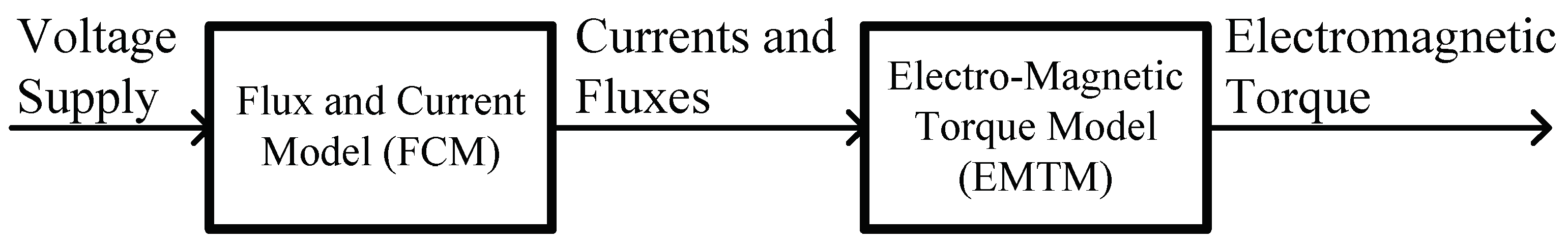
2.1. Prime Mover Modelling
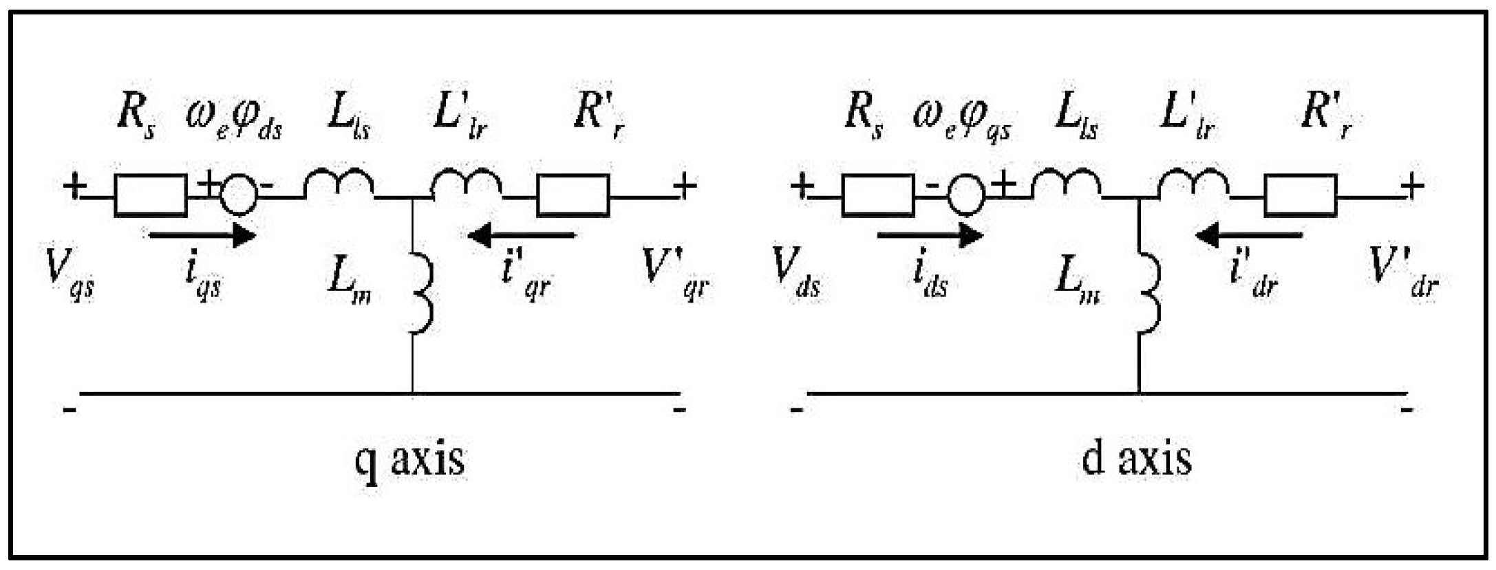
2.1.1. 3-Phase Induction Alternating Current (AC) Motor Block
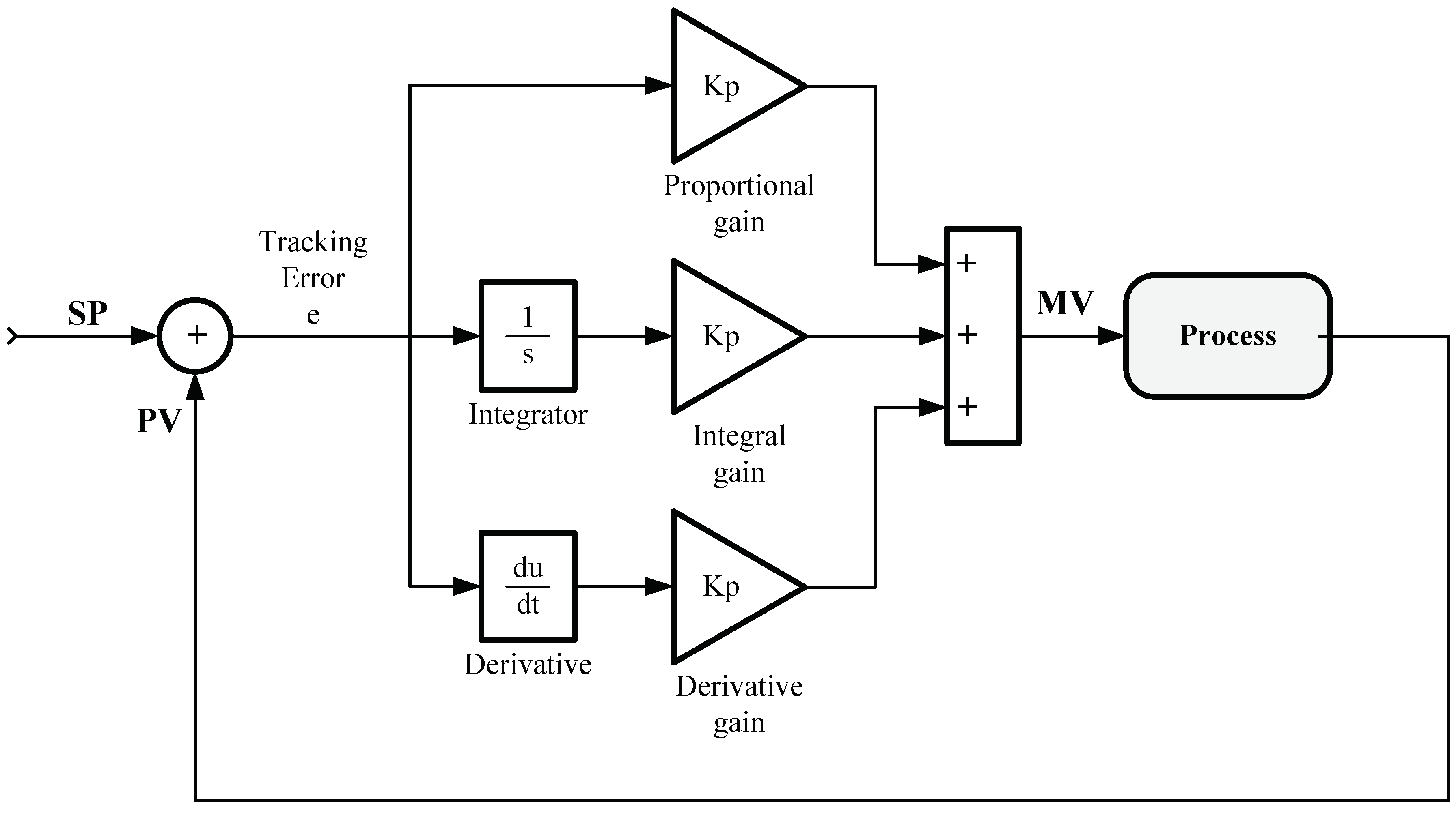
2.1.2. Proportional-Integral-Derivative (PID) Block and PID Controller Tuning
2.2. Propulsor Modelling
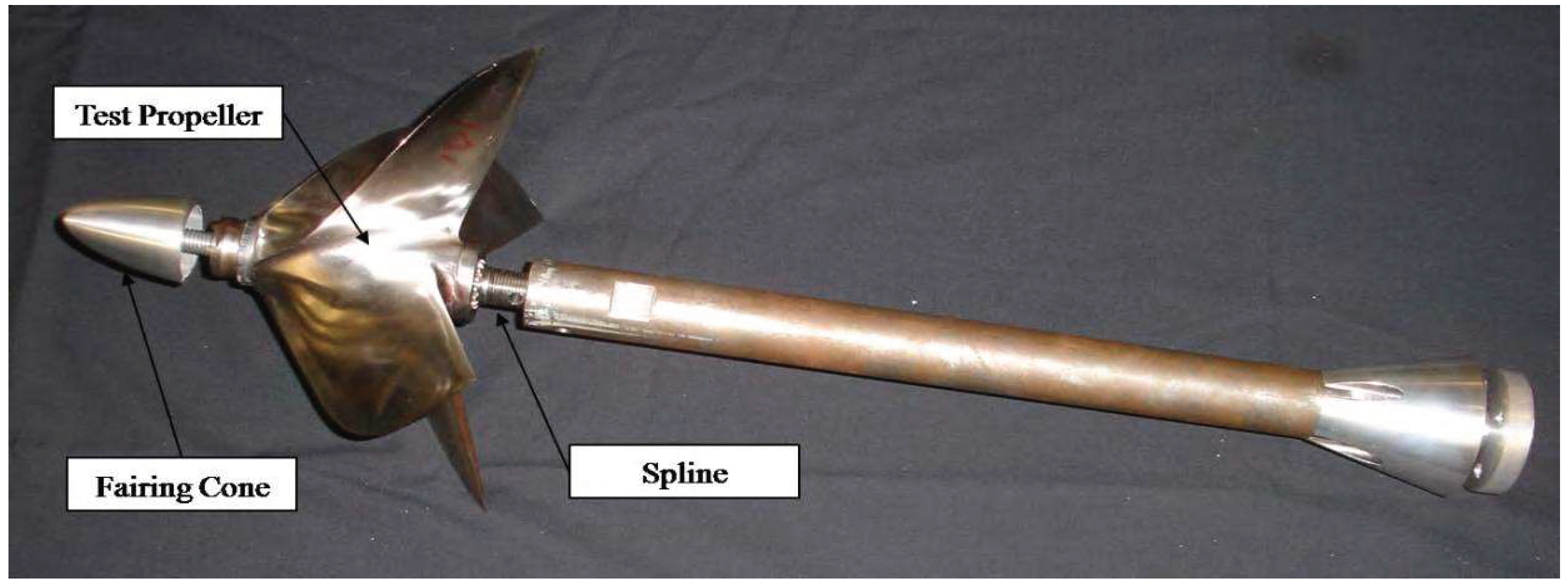
2.2.1. Towing Tank Data for Surface-Piercing Propeller
2.2.2. Configuration of Artificial Neural Networks (ANN)
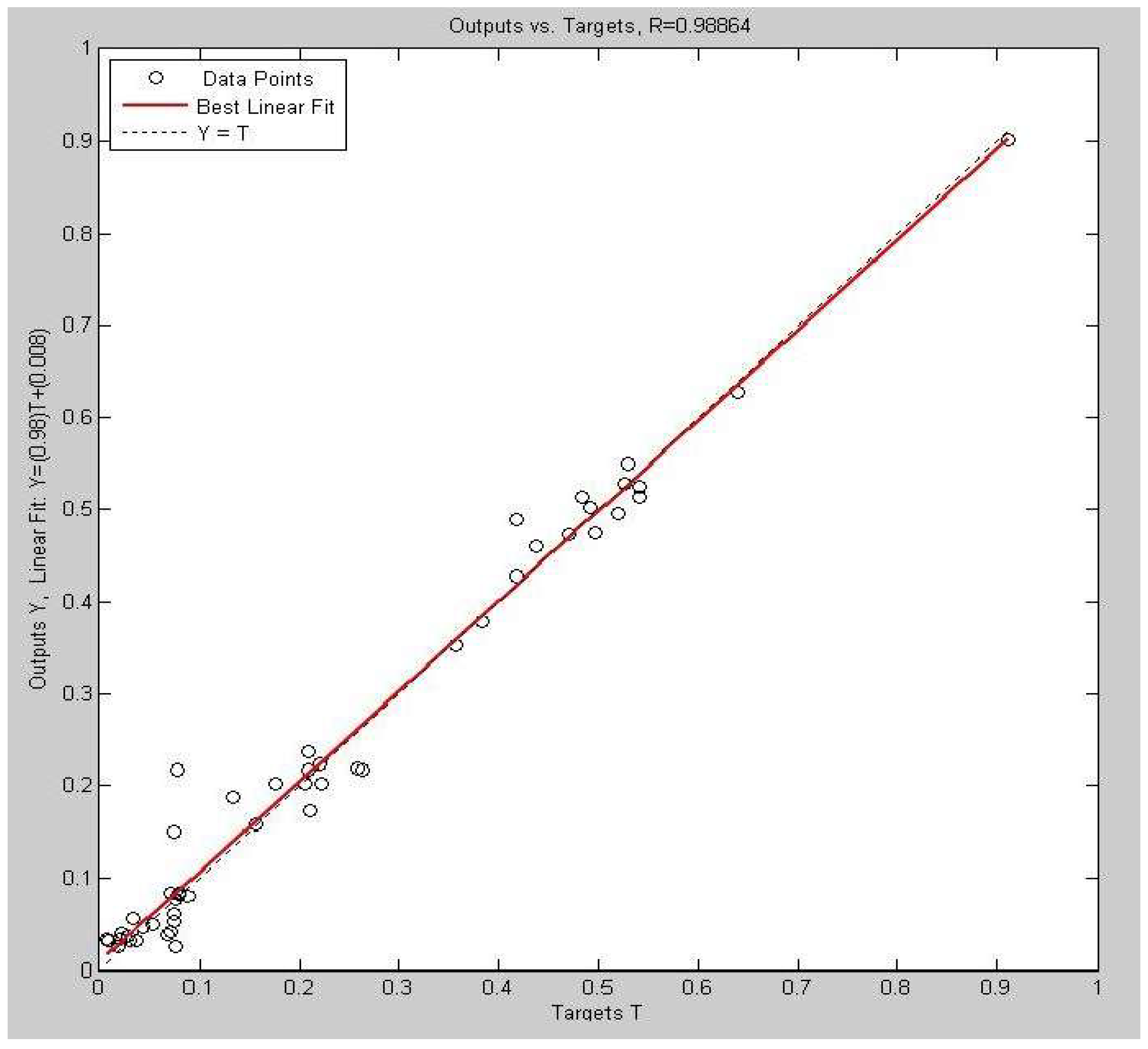
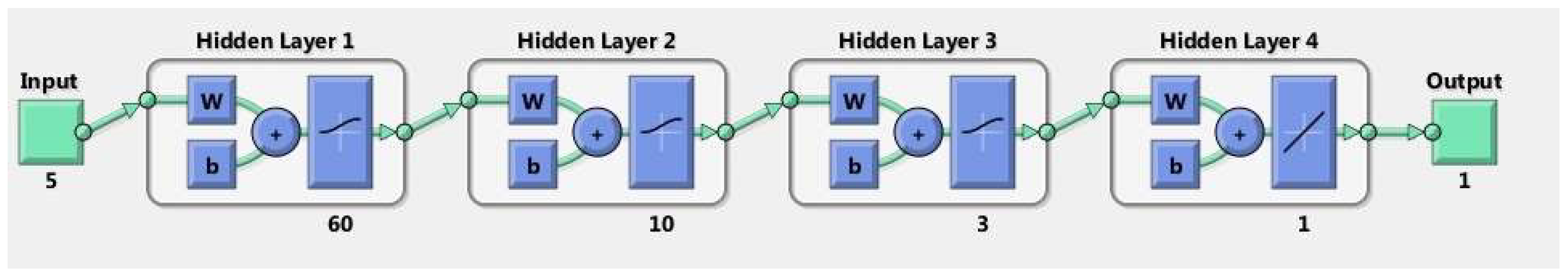
2.2.3. Thrust ANN
- Four layers;
- (60, 10, 3, 1) where 60 are the neurons of the 1st layer, 10 the neurons of the 2nd layer, 3 of the 3rd layer and 1 the number of neurons of the 4th;
- The transfer function for the first three layers is Logistic-Sigmoid (logsig) and pure linear for the last layer;
- The training function was selected as Conjugate Gradient Back-Propagation with Polak-Ribiere Updates (traincgp);
- The number of inputs are 5 () and number of outputs is 1 (Thrust: TSPP).
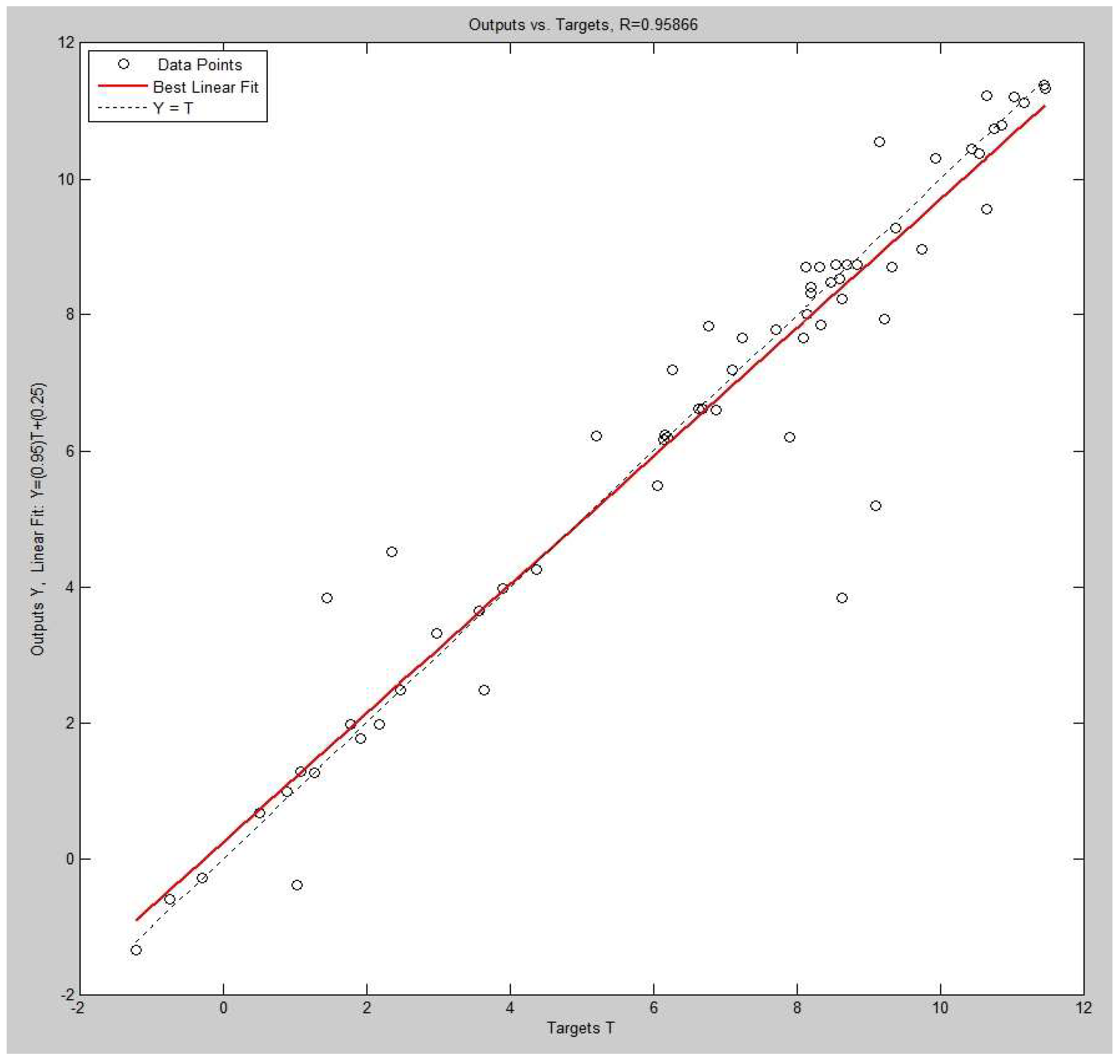
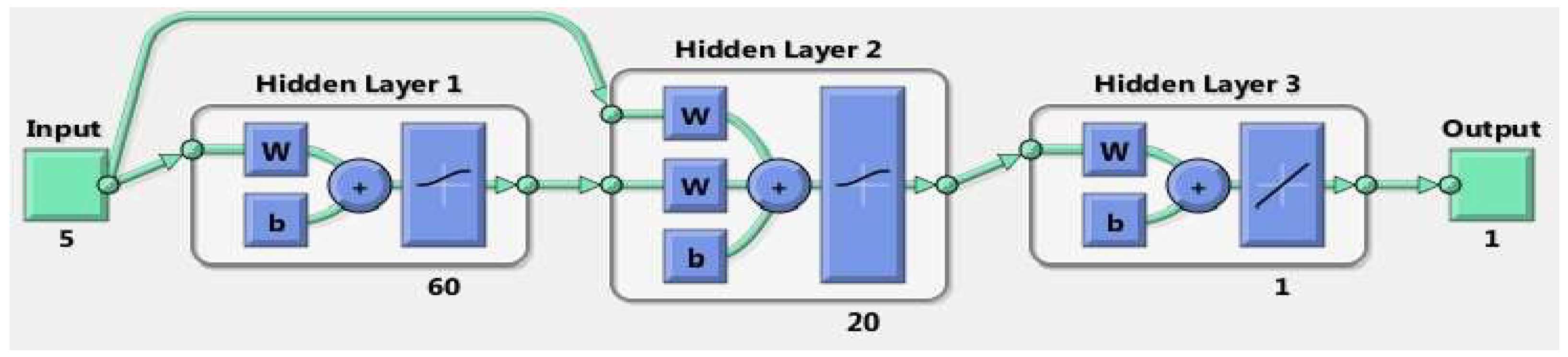
2.2.4. Torque ANN
- Three (3) layers;
- (60, 20, 1) where 60 are the neurons of the 1st layer, 20 the neurons of the 2nd layer and 1 the number of neurons of the 3rd;
- The transfer function for the first two layers is Logistic-Sigmoid (logsig) and pure linear (purelin) for the last layer;
- The training function was selected as Conjugate Gradient Back-Propagation with Polak–Ribiere Updates (traincgp);
- The number of inputs are 5 () and number of outputs is 1 (Torque: QSPP).
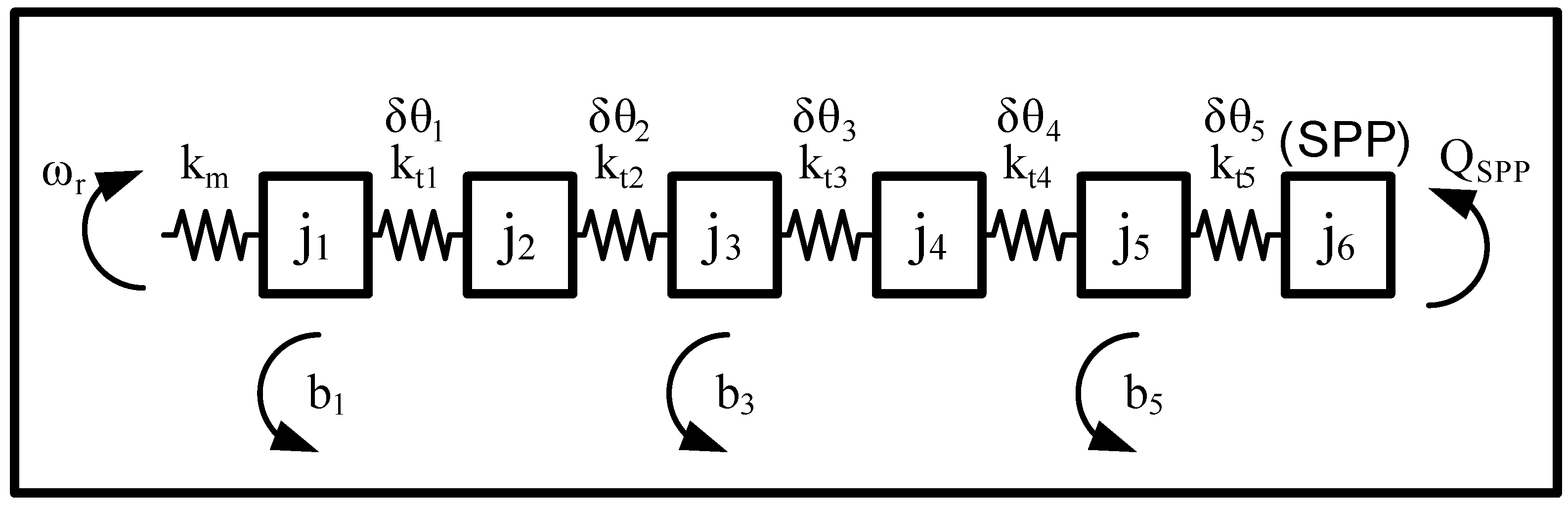
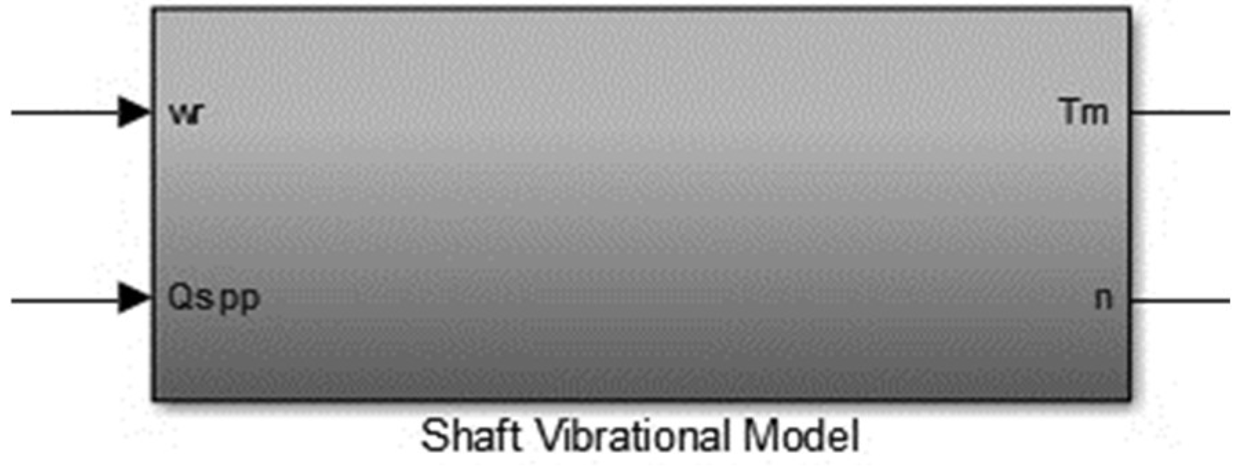
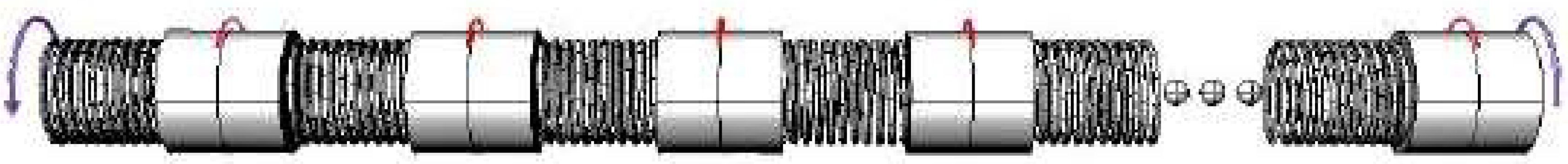
2.3. Propulsion Shaft Vibrational Modelling
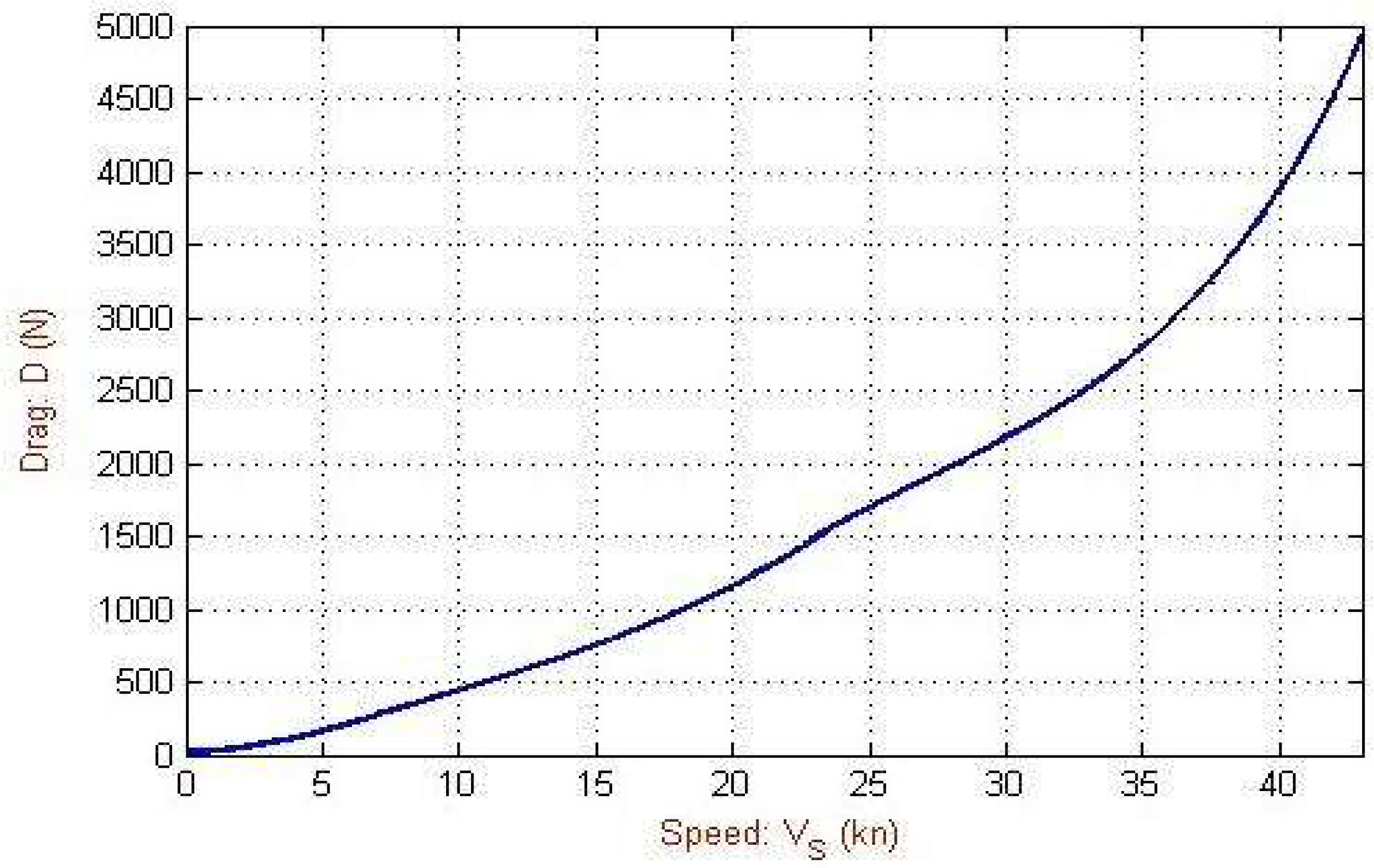
2.4. Equation for Linear Longitudinal Motion (Surge Dynamics)
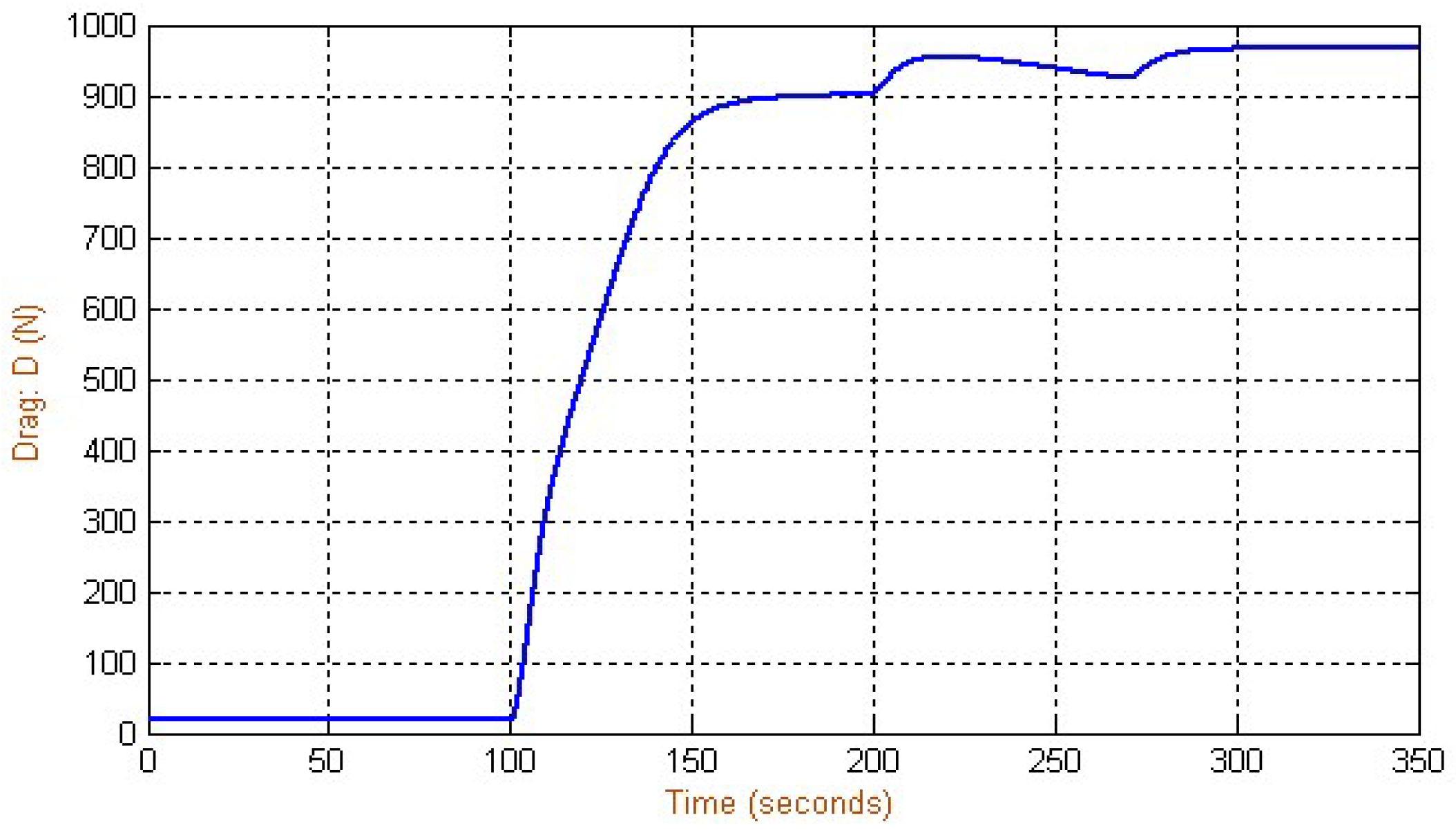
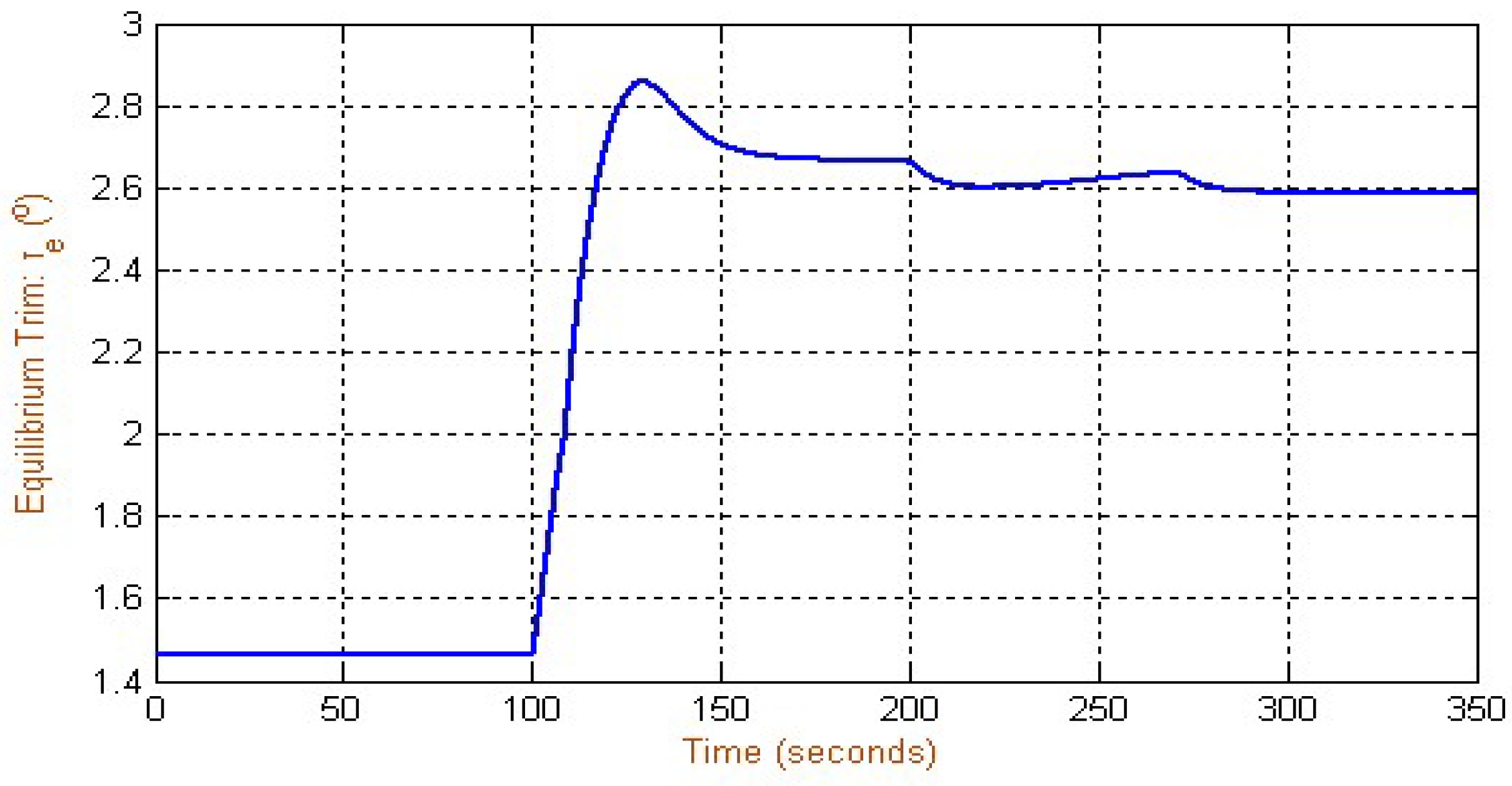
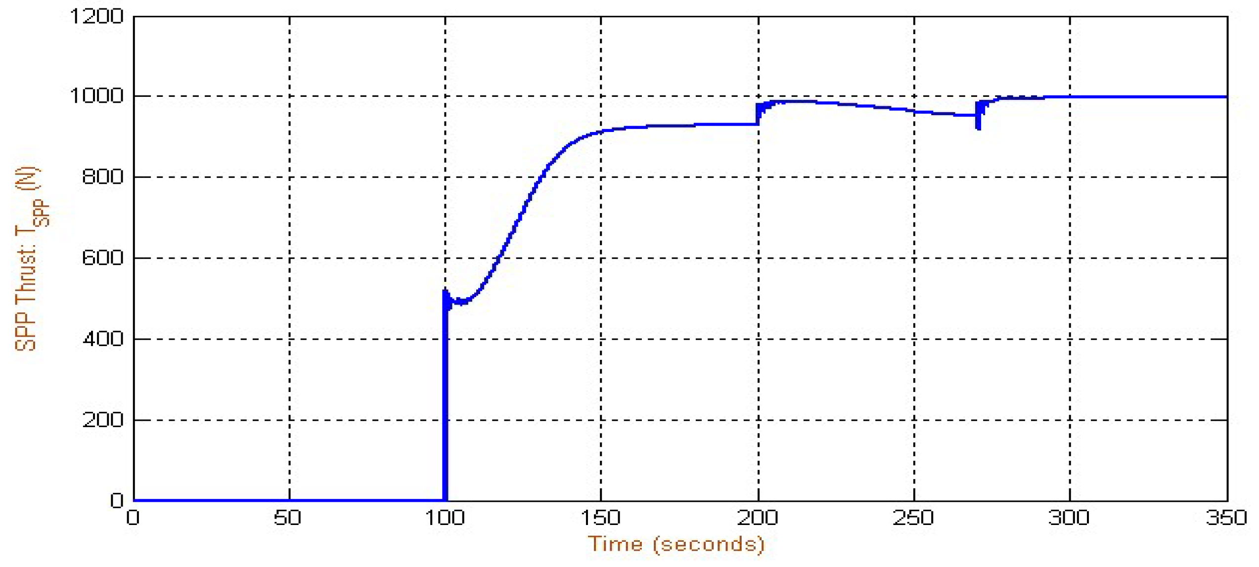
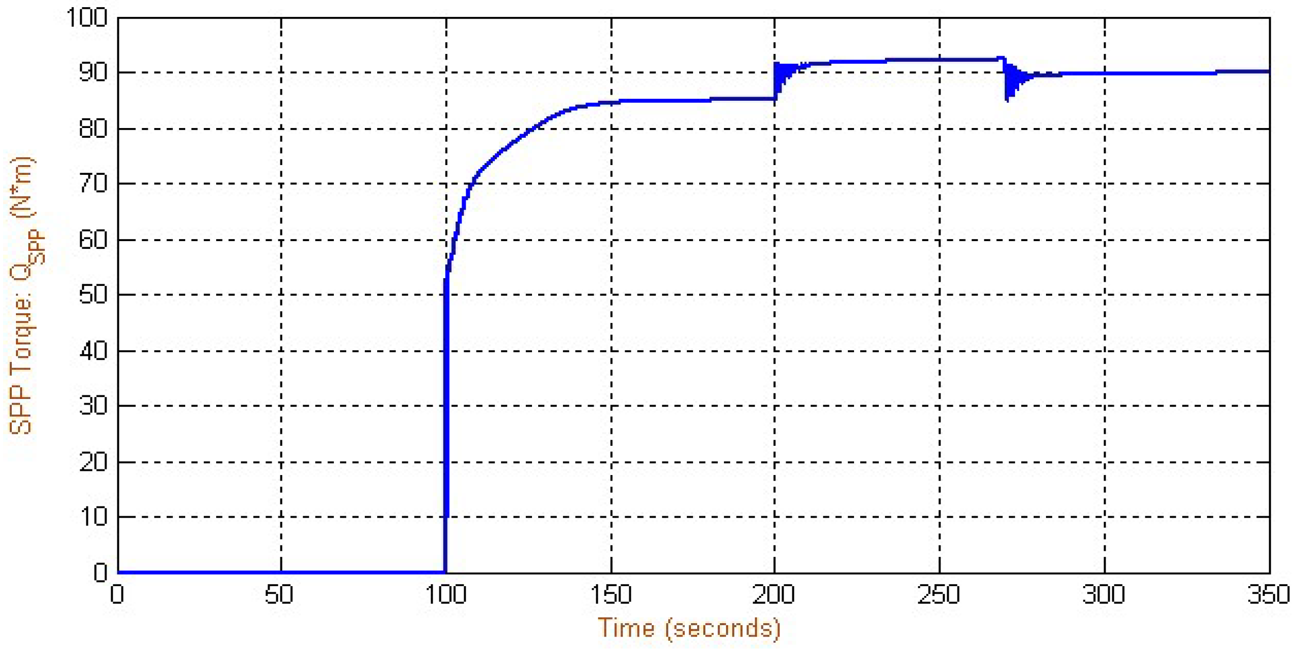
3. Results and Discussion
4. Conclusions
- (a)
- A computer simulation model for a watercraft propulsion system was developed that enables modular swapping of arbitrary subsystem models.
- (b)
- A systematic methodology to derive continuous, at least in the service range of interest, performance curves for conventional or unconventional marine thrusters was developed; then, the methodology was extended to include ship resistance and propulsion data for planing-hull vessels.
- (c)
- An electric motor subsystem model, a finite-difference dynamic model for the propeller shaft, as well as neural networks employed as empirical models for a surface-piercing propeller and planing-hull watercraft were refined and joined together to form an overall computer simulation model with modular usability and flexibility.
Author Contributions
Funding
Acknowledgments
Conflicts of Interest
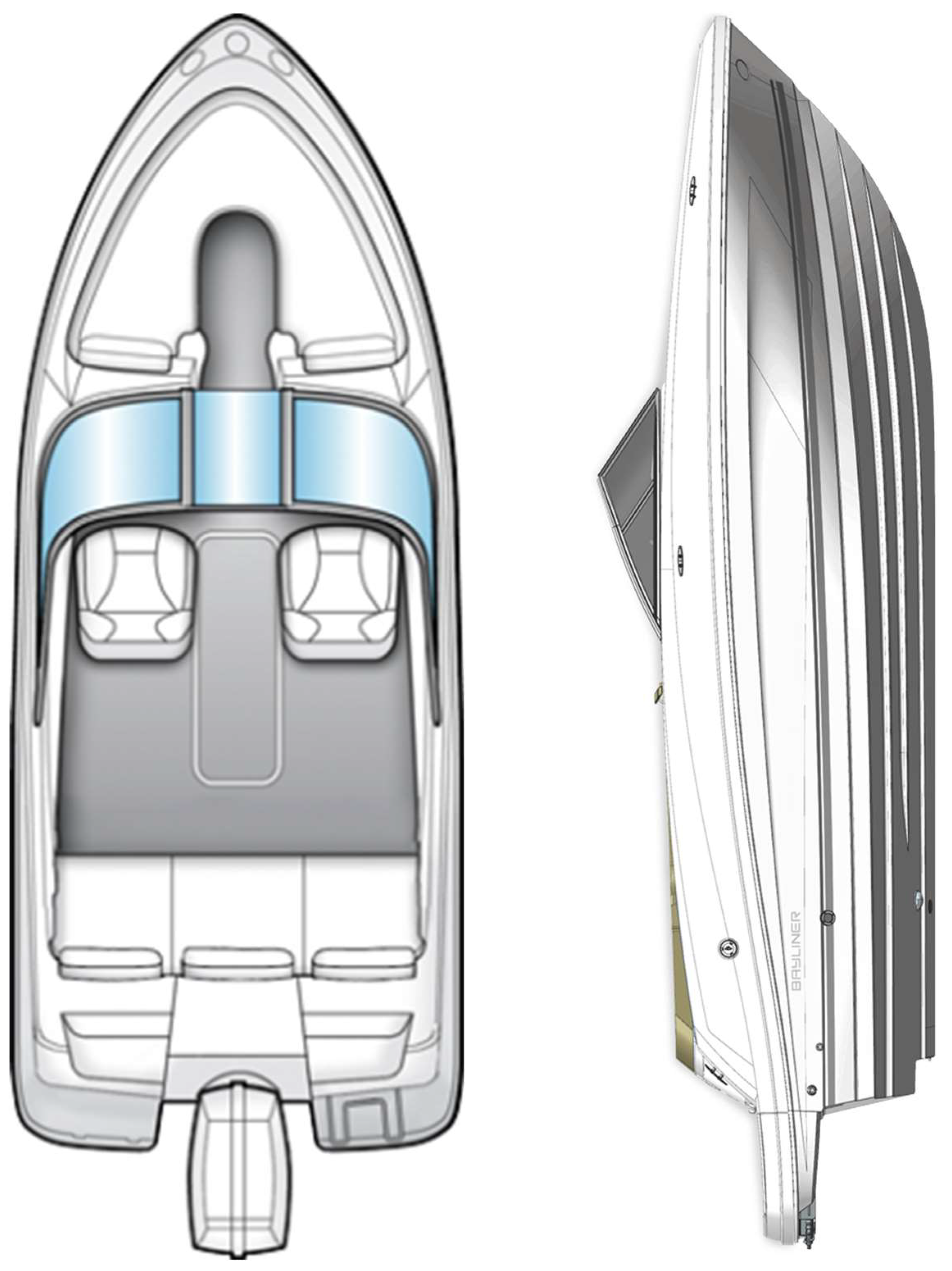
Appendix A. Configuration Specifics of Planing Hull

| Specifications | US | CE |
|---|---|---|
| Length overall (LOA) | 17’6” | 5.28 m |
| Beam | 6’11” | 2.09 m |
| Deadrise | 19° | 19° |
| Approx. weight w/standard engine | 1753 lbs. | 795 kg |
| Estimated draft | 2’11” | 89 m |
| Fuel capacity | 21 gal | 79.5 l |
| Max passenger capacity | 6 | 5 |
| Max passenger weight | 860 lbs. | 390 kg |

- (1)
- Generator set (outfitted with gasoline, diesel, natural gas or other type of engine as prime mover);
- (2)
- Battery bank;
- (3)
- Fuel cell system incl. hydrogen and oxygen storage;
- (4)
- Hybrid configuration(s).
References
- Marine Engineering; Harrington, R.L. (Ed.) Society of Naval Architects and Marine Engineers Press: Atlantic City, NJ, USA, 1992. [Google Scholar]
- Lorio, J.M. Open water testing of a surface piercing propeller with varying submergence, yaw angle and inclination angle. Master’s Thesis, Department of Ocean Engineering, Florida Atlantic University, Boca Raton, FL, USA, May 2010. [Google Scholar]
- Zisman, Z.S. On the Simulation of an All Electric Ship Powertrain Utilizing a Surface Piercing Propeller Via a Modular Main Propulsion Plant Model. Master’s Thesis, Department of Aerospace & Ocean Engineering, Virginia Tech, Blacksburg, VA, USA, May 2011. [Google Scholar]
- Von Ellenrieder, K. Open Water Towing Tank Testing of a Surface Piercing Propeller. Presented at the 29th American Towing Tank Conference, Annapolis, MD, USA, August 2010. [Google Scholar]
- Sul, S.-K. Control of Electric Machine Drive Systems; IEEE Press: Piscataway, NJ, USA, 2011. [Google Scholar]
- Xiros, N.I. Robust Control of Diesel Ship Propulsion; Springer: London, UK, 2002. [Google Scholar]
- Savitsky, D. Hydrodynamic design of planing hulls. Mar. Technol. 1964, 1, 71–95. [Google Scholar]
- Nazarov, A. On application of parametric method for design of planing craft. Presented at the 3rd Chesapeake Power Boat Symposium, Moscow, Russia, January 2012. [Google Scholar]


| AC Induction Motor Parameters 50 kW, 460 V(rms), 145 Hz, 4350 rpm, Squirrel Cage Rotor | |
|---|---|
| Stator Resistance (Rs) | 0.0641 Ω |
| Rotor Resistance (Rr) | 0.0441 Ω |
| Magnetizing Inductance (Lm) | 0.0100644 H |
| Total (Rotor & Stator) Inductance (Lls + Llr) | 0.0006449 H |
| Total Moment of Inertia (H) | 0.35 kg·m2 |
| Friction Factor (F) | 0.0025 Ν·m·s |
| Number of Pole Pairs (p) | 2 |
| PID Gain | Value |
|---|---|
| KP | 0.001 |
| KI | 0.015 |
| KD | 0.000 |
| Immersion Ratio IT (%) | Pitch Angle γ (Degrees) (Shaft Inclination Angle) | Yaw Angle ψ (Degrees) | Advance Ratio J (-) |
|---|---|---|---|
| 33 | 0, 7.5, 15 | 0, 15, 30 | 0.8 ∻ 1.9 |
| 50 | 0 | 0 | 0.8 ∻ 1.9 |
| Characteristic Type | Characteristic Value |
|---|---|
| Rotation | Left Handed |
| Pitch (P) | 0.465 m |
| Bore | Splined |
| Diameter (Dp) | 0.2464 m |
| Number of Blades (z) | 4 |
| Material | Stainless Steel |
| Number of Propellers (Np) | 2 |
| Matrix or Vector | Size |
|---|---|
| (60 × 5) | |
| (10 × 60) | |
| (3 × 10) | |
| (1 × 3) | |
| (60 × 1) | |
| (10 × 1) | |
| (3 × 1) | |
| (1 × 1) | |
| (60 × 1) | |
| (10 × 1) | |
| (3 × 1) | |
| (60 × 5) | |
| (20 × 5) | |
| (20 × 60) | |
| (20 × 1) | |
| (60 × 1) | |
| (20 × 1) | |
| (1 × 1) | |
| (60 × 1) | |
| (20 × 1) |
| Shaft Characteristic | Value |
|---|---|
| Shaft Length | 2 m |
| Number of Elements | 6 (-) (Propeller + 5 elements) |
| Number of Springs | 6 (-) |
| Shaft Diameter (Hollow Type) | Dout: 8 cm (outer) Din: 5 cm (inner) |
| Shaft-Primer Mover Flange | Df: 15 cm lf: 5 cm |
| Number of Bearings | 3 (-) |
| Shaft Material | Stainless Steel |
| Hull Characteristic | Value |
|---|---|
| LOA | 5.28 m |
| Bchine | 2.11 m |
| Deadrise (β) | 19° |
| Displacement (Δ) | 795 kg |
| LCG/VCG | 2.398 m/0.316 m |
| Inclination of Thrust Line Relative to Keel (e) | 0° |
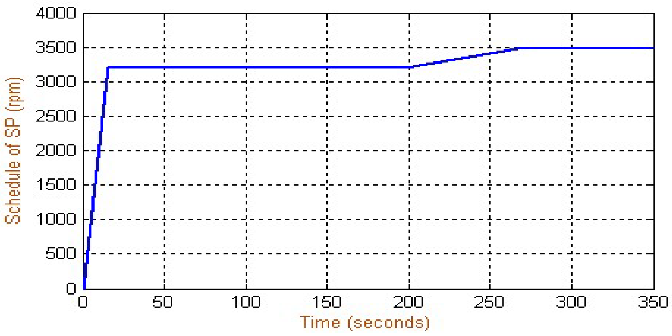
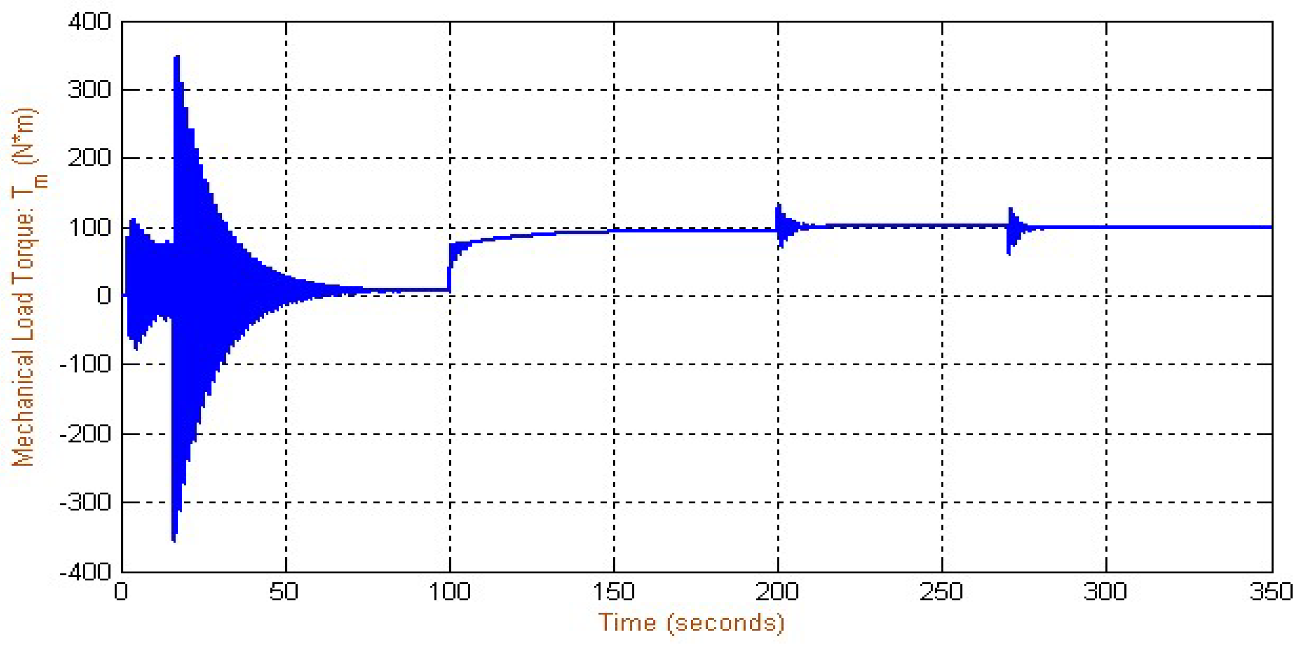
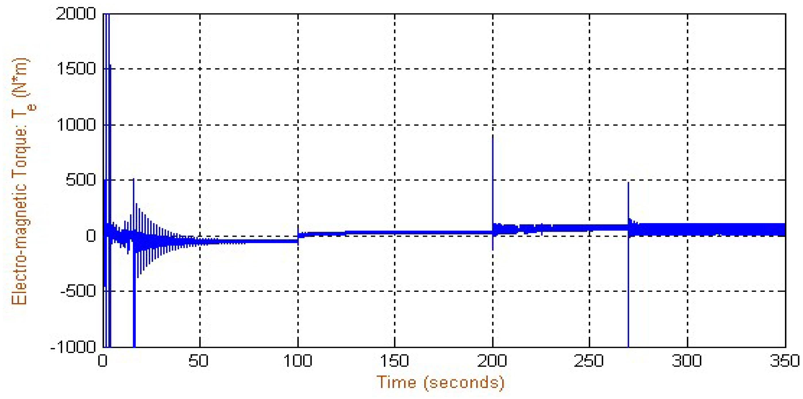
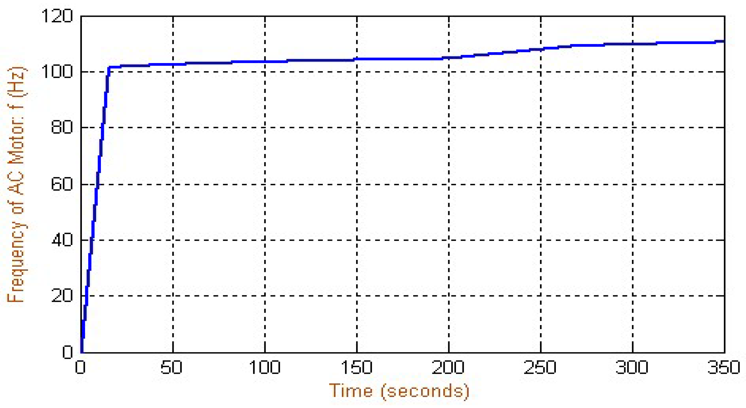
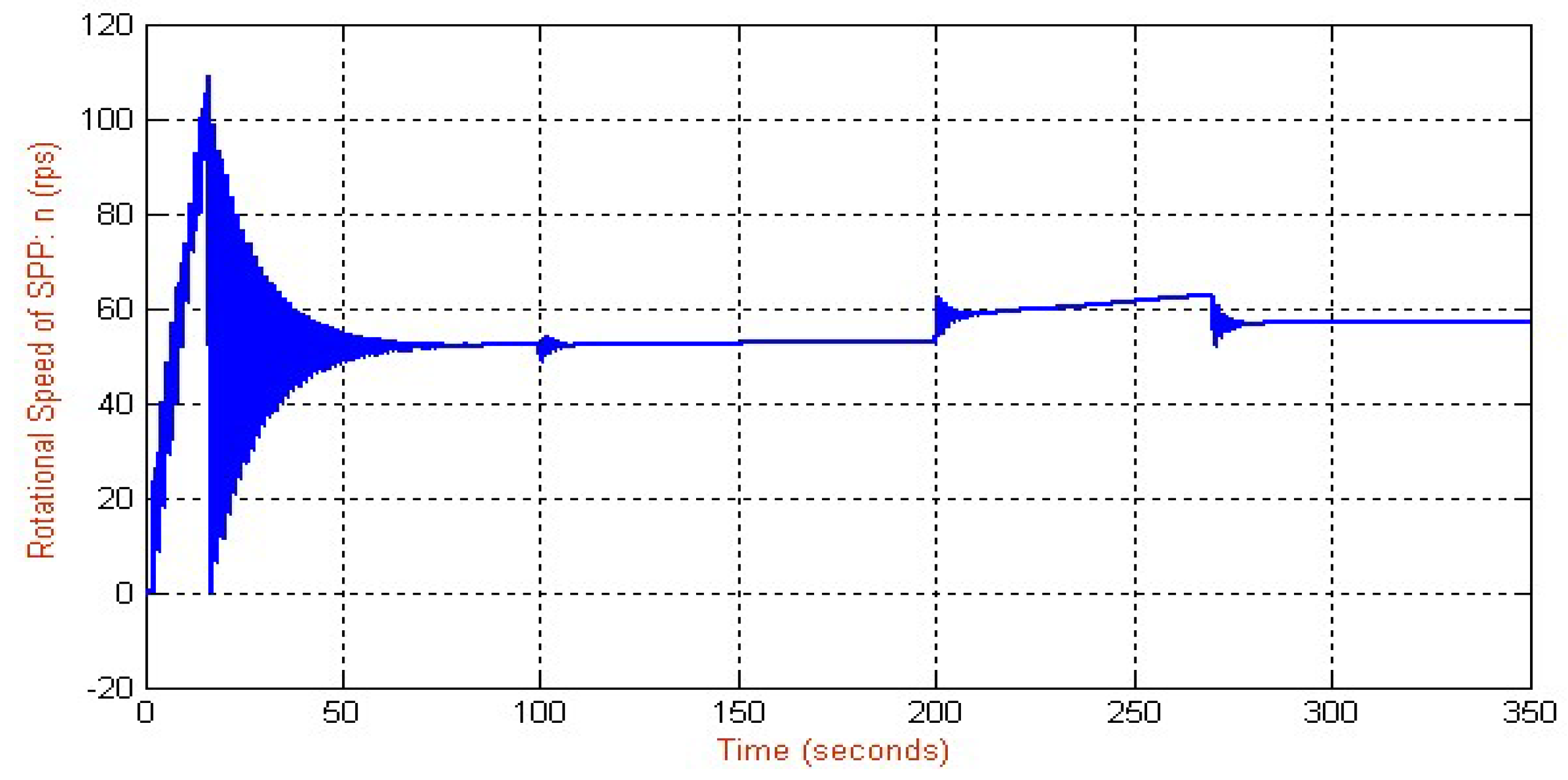
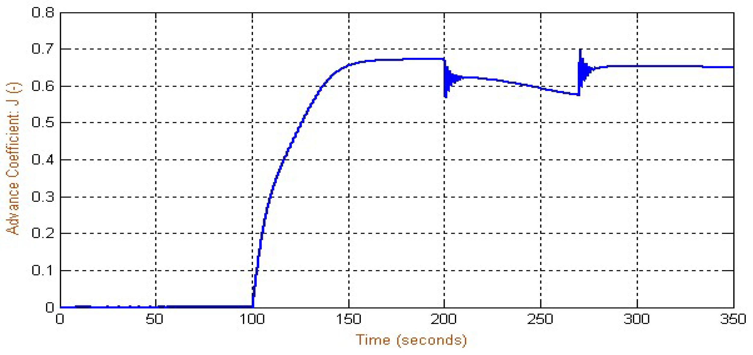
| Time (Seconds) | SP (rpm) (Rotor Speed Command) | Explanation |
|---|---|---|
| 0–16 | 0–3200 | Start and acceleration of AC motor |
| 16–100 | 3200 | Warm up of AC motor |
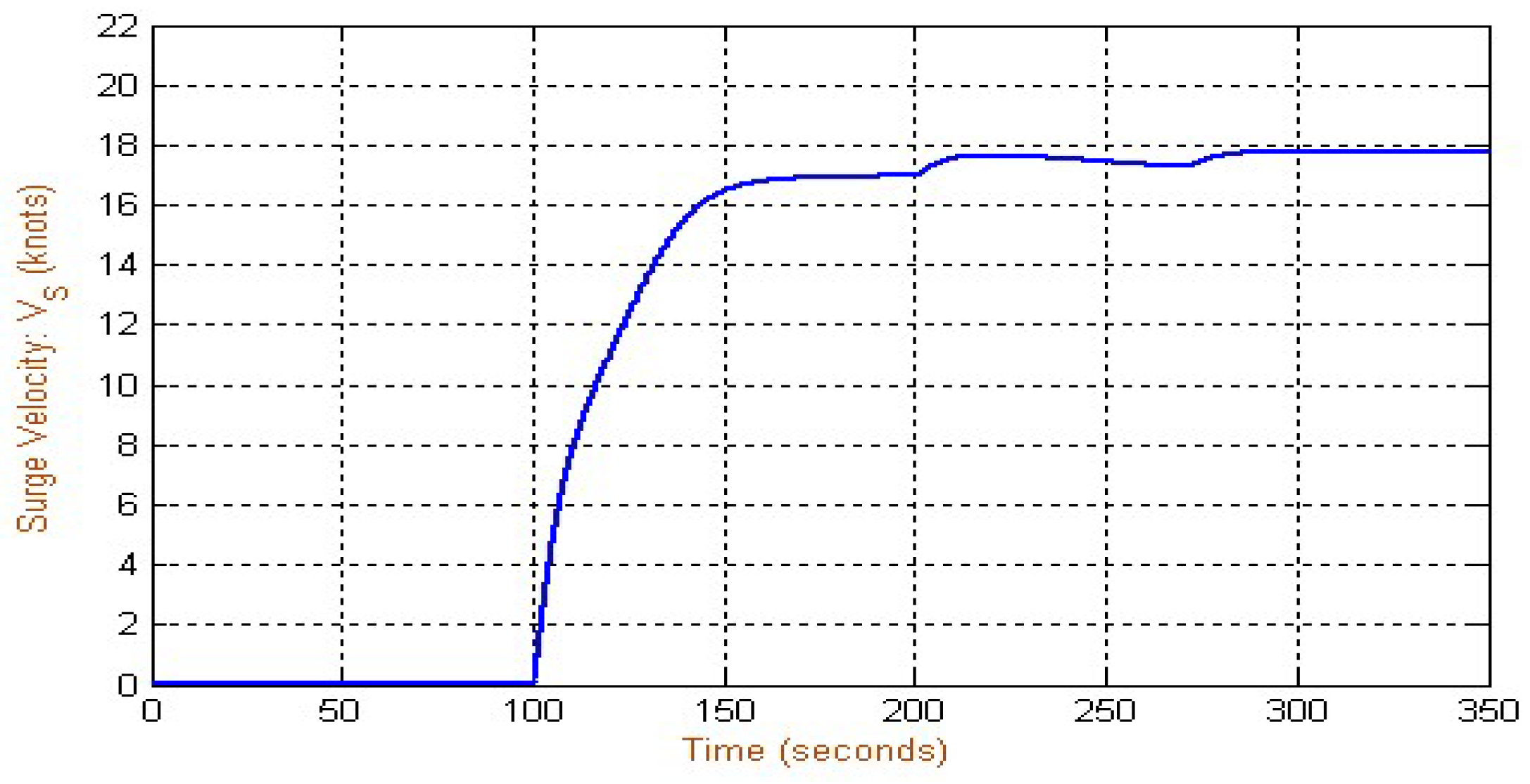
| 100 | 3200 | Connection of SPP to AC motor * |
| 100–165 | 3200 | Start and acceleration of the hull |
| 165–200 | 3200 | Steady state condition at VS = 17 kn (8.746 m/s) |
| 200–270 | 3200–3500 | Step (increase 300 rpm) of AC motor–Transient period of hull, propeller, AC motor |
| 270–350 | 3500 | Steady state condition at VS = 18 kn (9.260 m/s) |
© 2019 by the authors. Licensee MDPI, Basel, Switzerland. This article is an open access article distributed under the terms and conditions of the Creative Commons Attribution (CC BY) license (http://creativecommons.org/licenses/by/4.0/).
Share and Cite
Xiros, N.I.; Tzelepis, V.; Loghis, E.K. Modeling and Simulation of Planing-Hull Watercraft Outfitted with an Electric Motor Drive and a Surface-Piercing Propeller. J. Mar. Sci. Eng. 2019, 7, 49. https://doi.org/10.3390/jmse7020049
Xiros NI, Tzelepis V, Loghis EK. Modeling and Simulation of Planing-Hull Watercraft Outfitted with an Electric Motor Drive and a Surface-Piercing Propeller. Journal of Marine Science and Engineering. 2019; 7(2):49. https://doi.org/10.3390/jmse7020049
Chicago/Turabian StyleXiros, Nikolaos I., Vasileios Tzelepis, and Eleftherios K. Loghis. 2019. "Modeling and Simulation of Planing-Hull Watercraft Outfitted with an Electric Motor Drive and a Surface-Piercing Propeller" Journal of Marine Science and Engineering 7, no. 2: 49. https://doi.org/10.3390/jmse7020049