A Hamiltonian Surface-Shaping Approach for Control System Analysis and the Design of Nonlinear Wave Energy Converters

Abstract

The dynamic model of Wave Energy Converters (WECs) may have nonlinearities due to several reasons such as a nonuniform buoy shape and/or nonlinear power takeoff units. This paper presents the Hamiltonian Surface-Shaping (HSS) approach as a tool for the analysis and design of nonlinear control of WECs. The Hamiltonian represents the stored energy in the system and can be constructed as a function of the WEC’s system states, its position, and velocity. The Hamiltonian surface is defined by the energy storage, while the system trajectories are constrained to this surface and determined by the power flows of the applied non-conservative forces. The HSS approach presented in this paper can be used as a tool for the design of nonlinear control systems that are guaranteed to be stable. The optimality of the obtained solutions is not addressed in this paper. The case studies presented here cover regular and irregular waves and demonstrate that a nonlinear control system can result in a multiple fold increase in the harvested energy.

1. Introduction

One of the challenges in wave energy harvesting is the motion control. There has been significant developments for different control methods for WECs [1]. Most studies on the control of one-degree-of-freedom heaving WECs adopt a linear dynamic model—the Cummins’ equation [2]—which can be written as:

$${\displaystyle \left(m+\tilde{a}\right)\ddot{z}=F_{ex}+u-B_v\dot{z}-kz-{\int }_0^{\infty }{h}_r\left(\tau \right)\dot{z}(t-\tau )d\tau }$$

(1)

where z is the heave displacement, m is the buoy mass, k is the hydrostatic stiffness due to buoyancy, $\tilde{a}$ is the added mass, $F_{ex}$ is the excitation force, u is the control force, $B_v$ is a viscous damping coefficient, and $h_r$ is the radiation impulse response function (radiation kernel). The radiation term is called radiation force, $F_r$, and the buoyancy stiffness term is called the hydrostatic force.

There are multiple sources of possible nonlinearities in the WEC dynamic model though [3,4,5]. For example, if the buoy shape is not a vertical cylinder near the water surface, then the hydrostatic force will be nonlinear. The hydrodynamic forces can also be nonlinear in the case of large motion [6]. Control strategies that aim at maximizing the harvested energy usually increase the motion amplitude and, hence, increase the impact of these nonlinearities. The work in [6] presented a numerical implementation for nonlinear hydrodynamic forces at different levels from a full nonlinear model using Computational Fluid Dynamics (CFD) tools, linear models corrected by nonlinear Froude–Krylov force, as well as nonlinear viscous and hydrostatic forces. The Power Take Off (PTO) unit may have nonlinearities, as well [7]. The work in [8] points out that different WEC systems should choose only the relevant nonlinear effects to avoid unnecessary computational costs. For example, in the case of heaving point absorbers, the nonlinear Froude–Krylov force is essential, while the nonlinear diffraction and radiation can be neglected. The nonlinear viscous effects are weak as well for point absorbers [8], and the nonlinear PTO and mooring effects seem to be significant.

2. Linear WEC System

Consider a cylindrical buoy of radius r and height h in a regular wave, and assume that the buoy motion is small. The radiation damping force reduces to a linear damping for the case of a regular wave. The equation of motion in Equation (1) then becomes:

$${\displaystyle \left(m+\tilde{a}\right)\ddot{z}+(c+B_v)\dot{z}+kz=F_{ex}+u}$$

(2)

where c is the radiation damping coefficient. The harvested power is expressed as:

$$P\left(t\right)=-\left(u\right)\times \dot{z}\left(t\right)$$

(3)

For the system described above, the kinetic energy and potential energy functions can be written as:

$$T=\frac{1}{2}(m+\tilde{a}){\dot{z}}^2$$

(4)

$${\displaystyle V=-\int F_c\left(z\right)dz=\frac{k}{2}{z}^2}$$

(5)

where $F_c$ is the conservative forces. Although the added mass is not an actual mass, since it represents a force that contributes to the energy balance and this force is always $\tilde{a}\ddot{z}$, it can be included in computing T. Note that if the control force is two parts $u=u_c+u_{nc}$, where $u_c$ is a conservative force (e.g., a stiffness term) and $u_{nc}$ is a non-conservative force (e.g., a damping term), then $u_c$ can be included in the potential function V. To add that effect, assume that the potential of $u_c$ is $V_c=-\int u_{c}dz$. Hence:

$${\displaystyle V=\frac{k}{2}{z}^2+V_c}$$

(6)

The Hamiltonian function for the system is calculated as:

$$H=T+V$$

(7)

The Hamiltonian represents the stored energy, and the time derivative of the Hamiltonian is a power flow. The time derivative of Equation (7) can be written as:

$${\displaystyle \dot{H}=(m+\tilde{a})\ddot{z}\dot{z}+kz\dot{z}+{\dot{V}}_c}$$

(8)

Using Equations (2) and (8), we can write:

$$\begin{array}{ccc}\hfill \dot{H}& =& \dot{z}\left((m+\tilde{a})\ddot{z}+kz\right)+{\dot{V}}_c\hfill \end{array}$$

(9)

$$\begin{array}{ccc}& =& \dot{z}\left(F_{ex}-(c+B_v)\dot{z}+u\right)+{\dot{V}}_c\hfill \end{array}$$

(10)

The product $-\dot{z}u$ represents the power flow into the actuator, the PTO, as can be seen from Equation (3). Moreover, since the WEC is moving, the power flow is the summation of two parts: a conservative part ${\dot{V}}_c$ and a non-conservative part ${\dot{W}}_{nc}$.

$$-\dot{z}u={\dot{V}}_c+{\dot{W}}_{nc}$$

(11)

Hence, by substituting Equation (11) into Equation (10), we can write:

$$\begin{array}{ccc}\hfill \dot{H}& =& {\displaystyle \dot{z}\left(F_{ex}-(c+B_v)\dot{z}\right)+\left(\dot{z}u+{\dot{V}}_c\right)}\hfill \\ & =& {\displaystyle \dot{z}\left(F_{ex}-(c+B_v)\dot{z}\right)-{\dot{W}}_{nc}}\hfill \end{array}$$

(12)

A system is said to be conservative if $\dot{H}=0$ [9], which means the stored energy does not change over time. In other words, the power flow into the system balances the power flow out of the system at all times [10]. One would choose to have the WEC system behave like a conservative system, since in this case, the power flow from the wave into the WEC will go into the PTO (neglecting the power that gets dissipated in other forms such as hydrodynamic damping and structural dynamics). Note that in the case that $\dot{H}\ne 0$ and the system accumulates energy, it becomes unstable. By examining Equation (12) and recalling that ${\dot{W}}_{nc}=-\dot{z}{u}_{nc}$, it can be seen that for this WEC system to behave like a conservative system, the non-conservative part of the control (e.g., damping terms in u) must balance the summation of radiation damping force ($-c\dot{z}$), the excitation force, and the viscous damping force ($-B_v\dot{z}$), at all times. In such a case, the WEC will move in a perfect sinusoidal motion, as can be seen from Equation (9). Note that in this case, $V_c$ is due to a linear conservative force, which is a spring-type force, and hence, it changes the frequency of the sinusoidal motion. In fact, $V_c$ adjusts the natural frequency of the system to the resonance frequency.

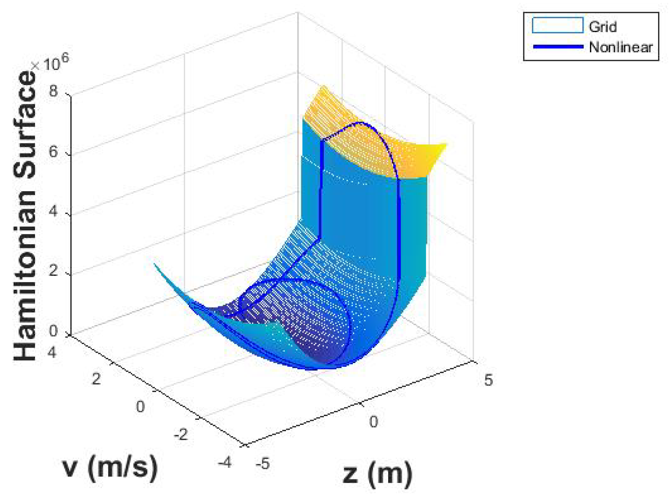
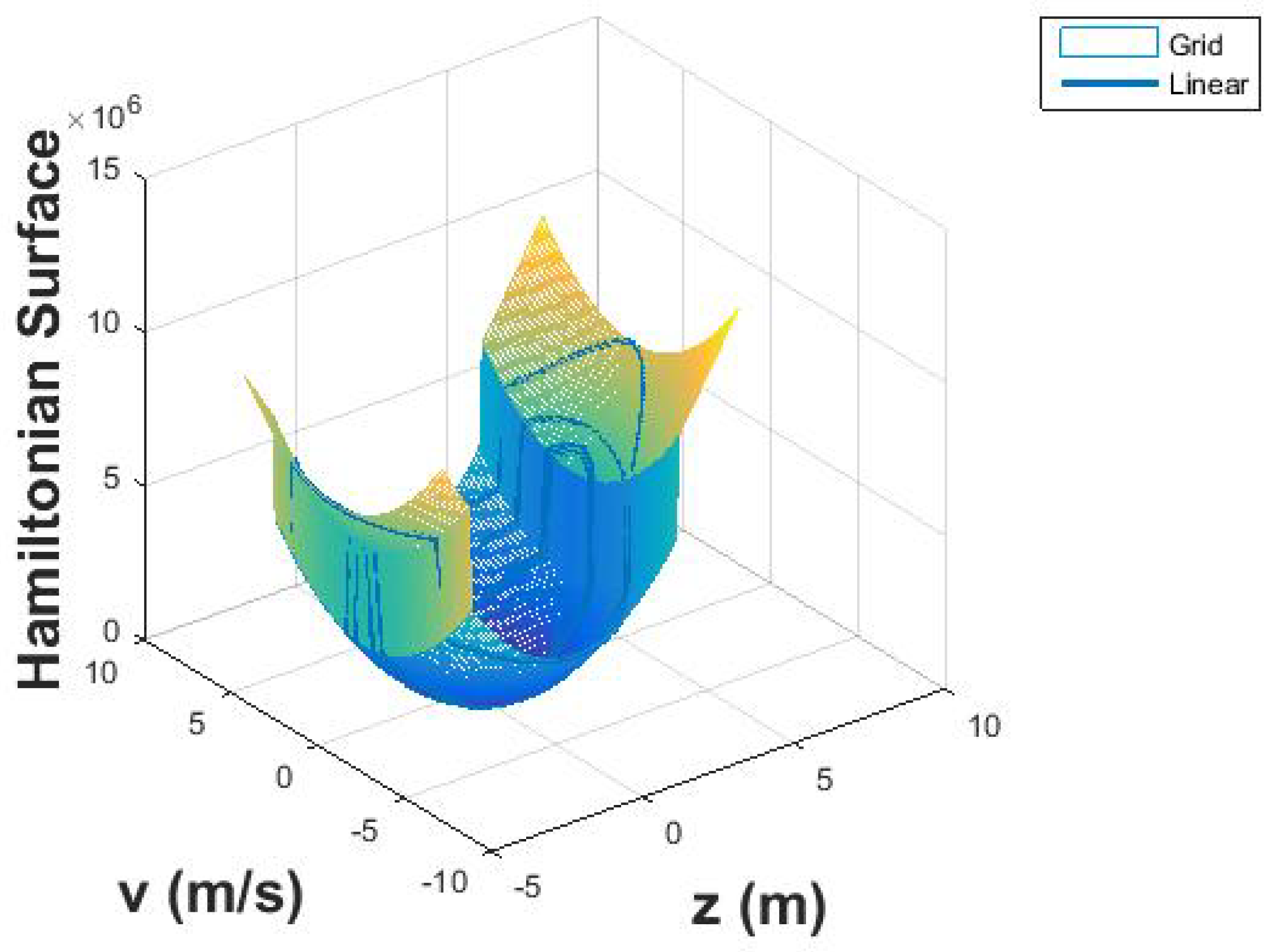
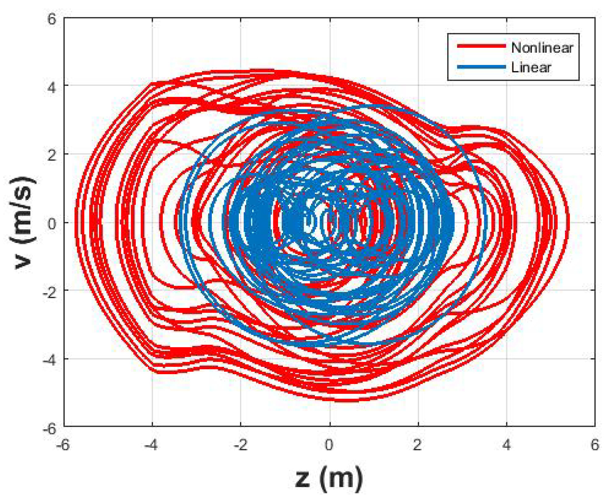
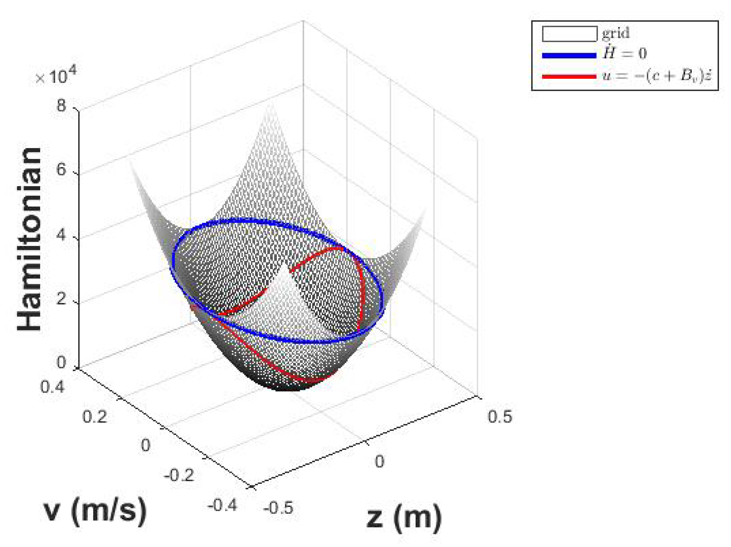
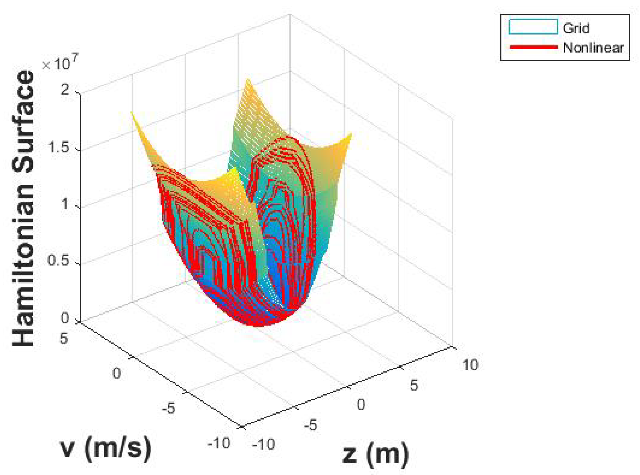
If we plot H versus z and $\dot{z}$ for the whole range of z and $\dot{z}$, we get the Hamiltonian surface, which is the locus for the states z and $\dot{z}$. Figure 1 shows an example of a Hamiltonian surface. As the system is moving over time, the states z and $\dot{z}$ will trace a trajectory on the Hamiltonian surface. In the case of a conservative system, H is constant ($\dot{H}=0$), which means that as the states change over time, the Hamiltonian value traces a closed trajectory (cycle) that is parallel to the $z-\dot{z}$ plane on the Hamiltonian surface. The time needed for the system to travel a full closed cycle is called the period of the cycle $\tau$. Note that the value of H on this cycle can be determined from the initial conditions of z and $\dot{z}$.

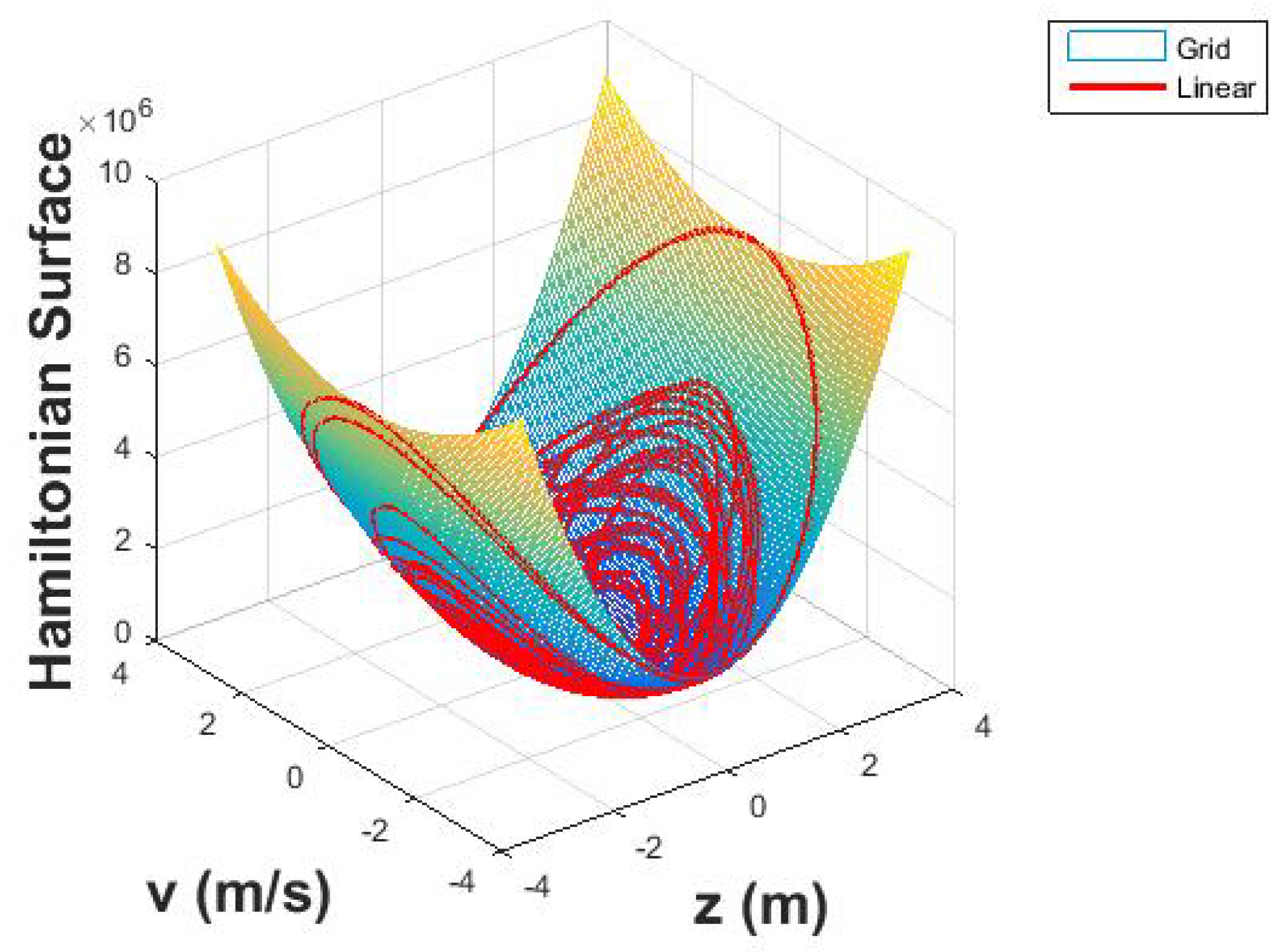
The works in [10,11] pointed out, however, that it is possible to integrate the power flow in Equation (8) to compute the work per cycle:

$${\displaystyle H_{cycle}={\oint }_{\tau }\dot{H}dt={\oint }_{\tau }\left((m+\tilde{a})\ddot{z}\dot{z}+kz\dot{z}+{\dot{V}}_c\right)dt}$$

(13)

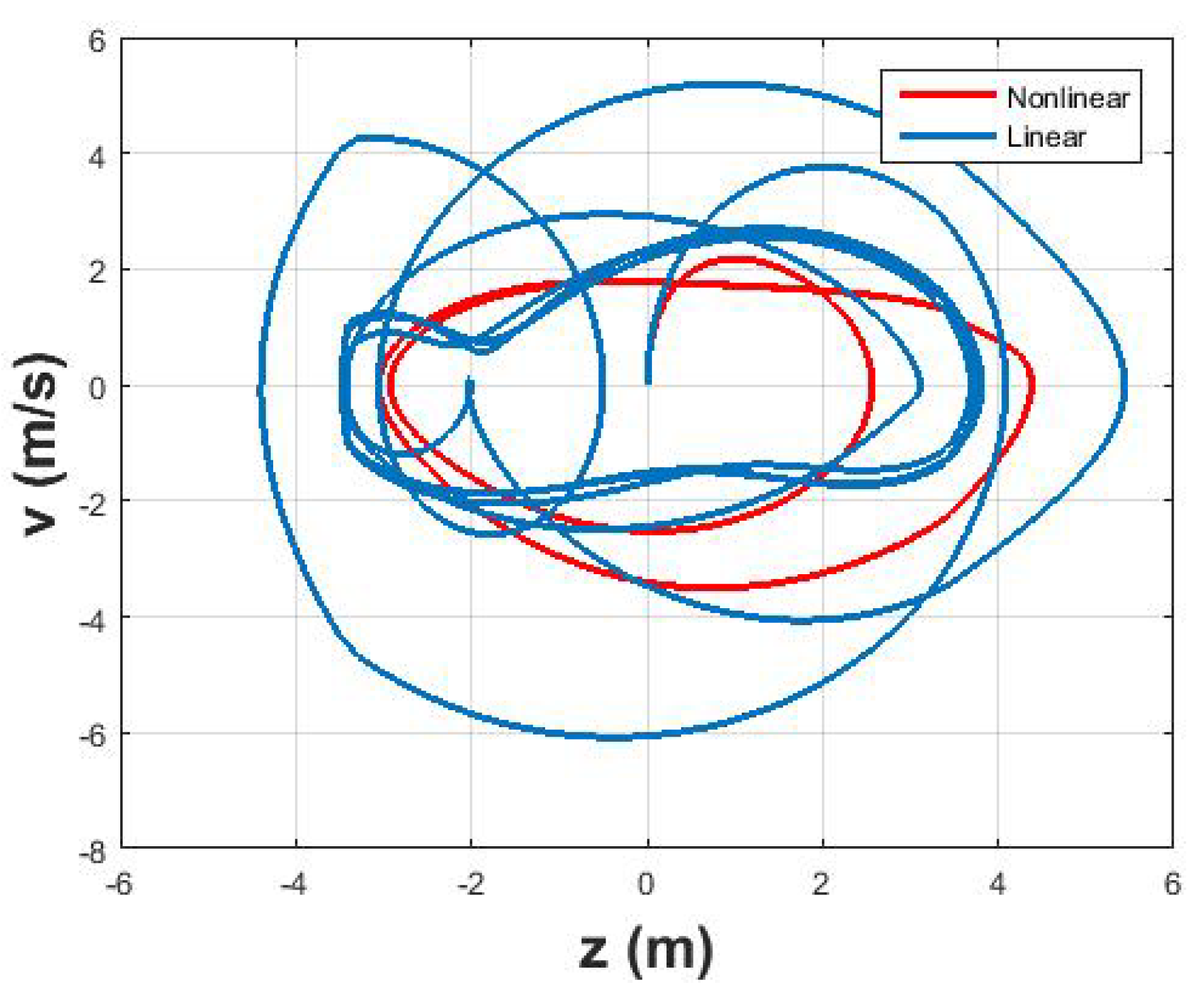
Hence, it is possible to design a control system that will achieve $H_{cycle}=0$ as opposed to $\dot{H}=0$. This condition allows more flexibility for the control design; the cyclic trajectory of the WEC is not constrained to be parallel to the $z-\dot{z}$ plane in this case; as long as the system returns to its initial state after some $\tau$ period of time. The two lines in Figure 1 represent two different controls for the same WEC. The WEC has a cylindrical buoy of radius $r=4.47$ m and a draft of $h=2r$ m, in a regular wave of $0.3$ m in amplitude and a period of nine seconds. No viscous damping is assumed. The $\dot{H}=0$ line represents the case when the non-conservative part of the control $u_{nc}$ cancels the summation of the radiation damping and excitation forces (see Equation (12)). The $H_{cycle}=0$ trajectory represents a case where a damping control is used of the form $u=-3\times {10}^4\dot{z}$ N. In other words, the difference between the two cases is due to the additional reactive power due to $V_c$. The initial states are assumed $z=0.317$ m and $\dot{z}=0.01$ m/second. Clearly in this case, there is no power flow balance at each point in time. As a result, the H value changes on the Hamiltonian surface along the trajectory and returns to its original value.

3. WEC in Large Motion

In the case of using nonlinear control, it is possible that the motion of the buoy grows large enough to make the buoy almost fully submerged or almost fully in the air. In such cases, the linear hydrodynamic model becomes invalid, and modeling of nonlinear hydrodynamics becomes inevitable. This is not the focus of this paper however. In this paper, we investigate the impact of having nonlinear terms in the equation of motion whether they appear due to nonlinear hydrodynamics, nonlinear hydrostatics, nonlinear damping, nonlinear control forces, or all of the above. Toward that end, the control force is here assumed in the form of a summation of two quantities:

$${\displaystyle u=u_l+{\tilde{u}}_c}$$

(14)

where $u_l$ is the linear part of the control and ${\tilde{u}}_c$ is the nonlinear control part. The harvested power can be expressed as:

$$P\left(t\right)=-({\tilde{u}}_c\left(t\right)+u_l)\times \dot{z}\left(t\right)=-u\times \dot{z}\left(t\right)$$

(15)

The nonlinear control part is assumed in the form:

$${\tilde{u}}_c=\sum _{i=1}^{Nc}{\alpha }_{c_i}{z}^i+\sum _{j=1}^{Mc}{\beta }_{c_j}{\dot{z}}^j$$

(16)

where ${\alpha }_{c_i}$ and ${\beta }_{c_j}$ are constant coefficients and $N_c$ and $M_c$ are the number of nonlinear terms that determine the order of control forces. The nonlinear control part ${\tilde{u}}_c$ does not have to be of the form presented in Equation (16); this form is selected as a case study in this paper.

The equation of motion of a WEC in large motion with nonlinear control takes the form:

$$\begin{array}{c}\hfill m\ddot{z}=F_{ex}+u+{\tilde{u}}_c+F_r+F_B\\ \hfill {\dot{\overrightarrow{x}}}_r=A_r{\overrightarrow{x}}_r+B_r\dot{z}\end{array}$$

(17)

where m is the buoy mass in addition to the added mass at infinite frequency, ${\overrightarrow{x}}_r$ represents the radiation states, $F_r$ is the radiation damping force, and $F_B$ is the buoyancy force.

The equation of motion, Equation (17), is derived assuming that the buoy does not leave the water, nor gets fully submerged in the water. In the case of nonlinear control presented in this paper, the motion of the buoy may grow large, and these two cases should not be excluded. Hence, the model in Equation (17) is modified as follows. A range $\left|z\right|<z_s$ is defined in which the model in Equation (17) is considered valid. The limit $z_s$ is selected based on the buoy dimensions and the wave height. When $\left|z\right|>z_s$, there are two possible cases. The first case is when $z>0$, that is when the buoy is (or very close to being) fully submerged under water. The second case is when $z<0$, that is when the buoy is (or very close to being) totally out of the water. In these two cases, the dynamic model in Equation (17) is not valid, and an approximate dynamic model is defined as follows:

Case 1 (z > 0):

The linear stiffness term becomes a constant $kh/2$. The excitation force is assumed to remain unchanged.

Case 2 (z < 0):

The buoy is out of the water, so there is no buoyancy force on it, meaning that $kz=-mg$, where g is the gravitational acceleration. There is no excitation force acting on the WEC; and there is no linear damping term on the left-hand side of Equation (17). The equation of motion reduces to $m\ddot{z}=mg+u_l+{\tilde{u}}_c$.

In this model, the radiation damping force $F_r$ takes the form:

$$F_r=\left\{\begin{array}{cc}{C}_r{\overrightarrow{x}}_r\hfill & \mathrm{if}\left|z\right|<z_s\hfill \\ C_r{\overrightarrow{x}}_r\hfill & \mathrm{if}\left|z\right|>z_s,z>0\hfill \\ 0\hfill & \mathrm{if}\left|z\right|>z_s,z<0\hfill \end{array}\right.$$

(18)

The buoyancy force $F_B$ can be calculated as:

$$F_B=\left\{\begin{array}{cc}mg-\rho g{V}_{b_s}\hfill & \mathrm{if}\left|z\right|<z_s\hfill \\ mg-\rho g{V}_b\hfill & \mathrm{if}\left|z\right|>z_s,z>0\hfill \\ mg\hfill & \mathrm{if}\left|z\right|>z_s,z<0\hfill \end{array}\right.$$

(19)

where $V_{b_s}$ is the submerged volume and $V_b$ is the total buoy volume. Please note that the slam force is not considered in this paper. Considering the approximate dynamic model (Cases 1 and 2) and Equations (17)–(19), the equation of motion in all the cases can be written in the state space form shown in Equation (20).

$$\left[\begin{array}{c}\dot{z}\\ \ddot{z}\\ {\dot{\overrightarrow{x}}}_r\end{array}\right]=\left[A\right]\left[\begin{array}{c}z\\ \dot{z}\\ {\overrightarrow{x}}_r\end{array}\right]+\frac{1}{m}\left[\begin{array}{c}0\\ u_l+{\tilde{u}}_c\\ 0\end{array}\right]+\frac{1}{m}\left[\begin{array}{c}0\\ F_{ex}\\ 0\end{array}\right]+\frac{1}{m}\left[\begin{array}{c}0\\ G\\ 0\end{array}\right]$$

(20)

where G is defined as:

$$G=\left\{\begin{array}{cc}0\hfill & \mathrm{if}\left|z\right|<z_s\hfill \\ -\frac{kh}{2}\hfill & \mathrm{if}\left|z\right|>z_s,z>0\hfill \\ mg\hfill & \mathrm{if}\left|z\right|>z_s,z<0\hfill \end{array}\right.$$

(21)

When $\left|z\right|>z_s$ and $z<0$, the excitation force vanishes, $F_{ex}=0$. The matrix $\left[A\right]$ in Equation (20) is defined as described in Equation (22).

$${\displaystyle \left[A\right]=\left\{\begin{array}{c}\left[\begin{array}{ccc}0& 1& 0\\ \frac{-k}{m}& 0& \frac{-C_r}{m}\\ 0& B_r& A_r\end{array}\right]\phantom{\infty }\mathrm{if}\left|z\right|<z_s\hfill \\ \left[\begin{array}{ccc}0& 1& 0\\ 0& 0& \frac{-C_r}{m}\\ 0& B_r& A_r\end{array}\right]\phantom{0}\mathrm{if}\left|z\right|>z_s\mathrm{and}z>0\hfill \\ \left[\begin{array}{ccc}0& 1& 0\\ 0& 0& 0\\ 0& B_r& A_r\end{array}\right]\phantom{0}\mathrm{if}\left|z\right|>z_s\mathrm{and}z<0\hfill \end{array}\right.}$$

(22)

Recall that $V_c=-\int u_{c}dz$. For the system described above, the potential energy in Equation (6) can be expressed as follows:

$${\displaystyle V=\left\{\begin{array}{cc}{\displaystyle \frac{k}{2}{z}^2-\sum _{i=1}^{Nc}\left({\displaystyle \frac{{\alpha }_{c_i}}{i+1}{z}^{i+1}}\right)}\hfill & \mathrm{if}\left|z\right|<z_s\hfill \\ \frac{kh}{2}z-{\displaystyle \sum _{i=1}^{Nc}}\left({\displaystyle \frac{{\alpha }_{c_i}}{i+1}{z}^{i+1}}\right)\hfill & \mathrm{if}\left|z\right|>z_s,z>0\hfill \\ -mgz-{\displaystyle \sum _{i=1}^{Nc}}\left({\displaystyle \frac{{\alpha }_{c_i}}{i+1}{z}^{i+1}}\right)\hfill & \mathrm{if}\left|z\right|>z_s,z<0\hfill \end{array}\right.}$$

(23)

Note that the $\beta$ terms are not shown in this equation since they are independent of z. The kinetic energy is computed as expressed in Equation (4). By substituting in Equation (7), the time derivative of the Hamiltonian can be written as:

$${\displaystyle \dot{H}=\left\{{\displaystyle \begin{array}{cc}{\displaystyle (m+\tilde{a})\ddot{z}\dot{z}+kz\dot{z}-{\displaystyle \sum _{i=1}^{Nc}}\left({\displaystyle {\alpha }_{c_i}{z}^i\dot{z}}\right)}\hfill & \mathrm{if}\left|z\right|<z_s\hfill \\ (m+\tilde{a})\ddot{z}\dot{z}+\frac{kh}{2}\dot{z}-{\displaystyle \sum _{i=1}^{Nc}}\left({\displaystyle {\alpha }_{c_i}{z}^i\dot{z}}\right)\hfill & \mathrm{if}\left|z\right|>z_s,z>0\hfill \\ (m+\tilde{a})\ddot{z}\dot{z}-mg\dot{z}-{\displaystyle \sum _{i=1}^{Nc}}\left({\displaystyle {\alpha }_{c_i}{z}^i\dot{z}}\right)\hfill & \mathrm{if}\left|z\right|>z_s,z<0\end{array}}\right.}$$

(24)

Using Equations (17) and (24), in the case when $\left|z\right|<z_s$, we can write:

$$\begin{array}{ccc}\hfill \dot{H}& =& {\displaystyle (m+\tilde{a})\ddot{z}\dot{z}+kz\dot{z}-\sum _{i=1}^{Nc}\left({\displaystyle {\alpha }_{c_i}{z}^i\dot{z}}\right)}\hfill \end{array}$$

$$\begin{array}{cccc}& & =& \dot{z}\left((m+\tilde{a})\ddot{z}+kz-\sum _{i=1}^{Nc}\left({\displaystyle {\alpha }_{c_i}{z}^i}\right)\right)\hfill \end{array}$$

(25)

$$\begin{array}{cccc}& & =& \dot{z}\left(F_{ex}-(c+B_v)\dot{z}+{\displaystyle \sum _{j=1}^{Mc}}\left({\displaystyle {\beta }_{c_j}{\dot{z}}^j}\right)\right),\left|z\right|<z_s\hfill \end{array}$$

(26)

Similarly for the other two regions ($\left|z\right|>z_s$), we can write:

$$\begin{array}{c}\hfill \begin{array}{ccc}\dot{H}\hfill & =\hfill & \dot{z}\left(F_{ex}-(c+B_v)\dot{z}+\sum _{j=1}^{Mc}\left({\displaystyle {\beta }_{c_j}{\dot{z}}^j}\right)\right)\hfill \end{array},\left|z\right|>z_s,z>0\end{array}$$

(27)

$$\begin{array}{c}\hfill \begin{array}{ccc}\dot{H}\hfill & =\hfill & \dot{z}\sum _{j=1}^{Mc}{\beta }_{c_j}{\dot{z}}^j\hfill \end{array},\left|z\right|>z_s,z<0\end{array}$$

(28)

Using Equations (24) and (25), then the work per cycle can be computed as:

$$H_{cycle}={\oint }_{\tau }\dot{H}dt=\left\{{\displaystyle \begin{array}{cc}{\displaystyle {\oint }_{\tau }\dot{z}\left((m+\tilde{a})\ddot{z}+kz-{\displaystyle \sum _{i=1}^{Nc}}\left({\displaystyle {\alpha }_{c_i}{z}^i}\right)\right)dt}\hfill & \mathrm{if}\left|z\right|<z_s\hfill \\ {\oint }_{\tau }\dot{z}\left((m+\tilde{a})\ddot{z}+kh/2-{\displaystyle \sum _{i=1}^{Nc}}\left({\displaystyle {\alpha }_{c_i}{z}^i}\right)\right)dt\hfill & \mathrm{if}\left|z\right|>z_s,z>0\hfill \\ {\oint }_{\tau }\dot{z}\left((m+\tilde{a})\ddot{z}-mg-{\displaystyle \sum _{i=1}^{Nc}}\left({\displaystyle {\alpha }_{c_i}{z}^i}\right)\right)dt\hfill & \mathrm{if}f\left|z\right|>z_s,z<0\hfill \end{array}}\right.$$

(29)

Also using Equations (26)–(28), the work per cycle can be computed as:

$${\displaystyle H_{cycle}={\oint }_{\tau }\dot{H}dt=\left\{\begin{array}{cc}{\displaystyle {\oint }_{\tau }\dot{z}\left(F_{ex}-(c+B_v)\dot{z}+{\displaystyle \sum _{j=1}^{Mc}}\left({\displaystyle {\beta }_{c_j}{\dot{z}}^j}\right)\right)dt}\hfill & \mathrm{if}\left|z\right|<z_s\hfill \\ {\oint }_{\tau }\dot{z}\left(F_{ex}-(c+B_v)\dot{z}+{\displaystyle \sum _{j=1}^{Mc}}\left({\displaystyle {\beta }_{c_j}{\dot{z}}^j}\right)\right)dt\hfill & \mathrm{if}\left|z\right|>z_s,z>0\\ {\oint }_{\tau }\dot{z}{\displaystyle \sum _{j=1}^{Mc}}{\beta }_{c_j}{\dot{z}}^{j}dt\hfill & \mathrm{if}\left|z\right|>z_s,z<0\end{array}\right.}$$

(30)

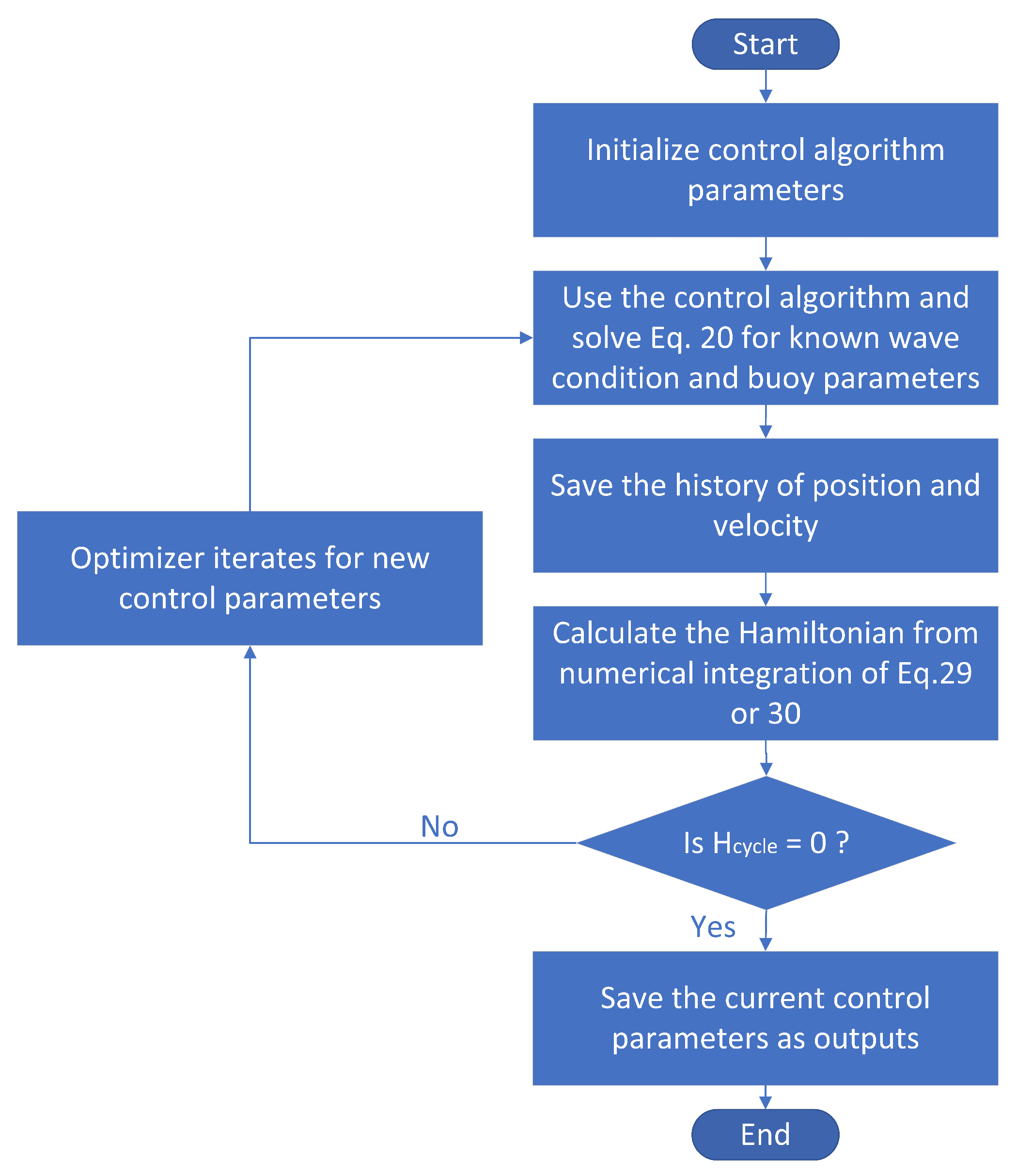
Equations (29) and (30) can be used for control design and for simulation of this nonlinear WEC system. Depending on the form that $H_{cycle}$ has, the equation of motion can be selected such that $H_{cycle}=0$ over some period $\tau$. This will guarantee stability of the control system design. The coefficients ${\alpha }_{c_i}$ should be selected such that $H_{cycle}=0$ in Equation (29) over the same period $\tau$. Using the selected values for ${\alpha }_{c_i}$ and ${\beta }_{c_j}$, the system can be simulated via numerical integration of Equations (24) and (26)–(28), simultaneously. A conceptual diagram of this process is shown in Figure 2. Section 4 presents an illustrative case study.

4. Case Study 1: Prescribed Hamiltonian

As discussed in the previous sections, it is possible to design a controller that satisfies the requirement of $H_{cycle}=0$ over some period $\tau$. This would be of interest in wave energy conversion especially in the case of regular waves since the wave repeats itself at a regular rate; and hence, it is intuitive that a control system that brings the WEC to some initial state at the same rate would be suitable. Consider a cylindrical buoy of radius $4.47$ m and a draft of $8.94$ m, in a regular wave of period $P_w=9$ s. Assume that:

$$H\left(t\right)=z^2\left(t\right)+{\dot{z}}^2\left(t\right)⟹\dot{H}=2\dot{z}\left(z+\ddot{z}\right)$$

(31)

Next, the control coefficients ${\alpha }_{c_i}$ and ${\beta }_{c_i}$ are chosen such that the selected Hamiltonian trajectory over time, Equation (31), is achieved. To do that, we start by substituting for $\dot{H}$ from Equation (31) into Equation (24) to get:

$$2\left(z+\ddot{z}\right)=\left\{{\displaystyle \begin{array}{cc}{\displaystyle (m+\tilde{a})\ddot{z}+kz-\sum _{i=1}^{Nc}\left({\displaystyle {\alpha }_{c_i}{z}^i}\right)}\hfill & \mathrm{if}\left|z\right|<z_s\hfill \\ (m+\tilde{a})\ddot{z}+\frac{kh}{2}-{\displaystyle \sum _{i=1}^{Nc}}\left({\displaystyle {\alpha }_{c_i}{z}^i}\right)\hfill & \mathrm{if}\left|z\right|>z_s,z>0\\ (m+\tilde{a})\ddot{z}-mg-{\displaystyle \sum _{i=1}^{Nc}}\left({\displaystyle {\alpha }_{c_i}{z}^i}\right)\hfill & \mathrm{if}\left|z\right|>z_s,z<0\end{array}}\right.$$

(32)

Then, Equation (32) can be solved for the control coefficients ${\alpha }_{c_i}$, $z\left(t\right)$, and $\dot{z}\left(t\right)$; this can be achieved by solving a least squares error to minimize $H_{cycle}^2$, for a given number of coefficients $N_c$. In this case, the optimizer iterates on different values for the coefficients ${\alpha }_{c_i}$, where in each iteration, Equation (32) is solved for $z\left(t\right)$ and $\dot{z}\left(t\right)$, and the objective function value $H_{cycle}^2$ is computed for this iteration. Once obtained, $z\left(t\right)$ and $\dot{z}\left(t\right)$ are substituted in Equations (26)–(28) to solve for the coefficients ${\beta }_{c_i}$. In fact, in this illustrative example, where we assumed a shape for the Hamiltonian given by Equation (31), we do not need to solve for the coefficients ${\beta }_{c_i}$; rather, it is possible to set a variable $u_d\left(t\right)={\sum }_{i=1}^{Nc}{\beta }_{c_i}{\dot{z}}^i$ and solve for $u_d\left(t\right)$ in Equations (26)–(28) to get:

$$u_d\left(t\right)=\left\{\begin{array}{cc}2\left(z+\ddot{z}\right)-\left(F_{ex}-(c+B_v)\dot{z}\right)\hfill & \mathrm{if}\left|z\right|<z_s\hfill \\ 2\left(z+\ddot{z}\right)-\left(F_{ex}-(c+B_v)\dot{z}\right)\hfill & \mathrm{if}\left|z\right|>z_s,z>0\\ 2\left(z+\ddot{z}\right)\hfill & \mathrm{if}\left|z\right|>z_s,z<0\end{array}\right.$$

(33)

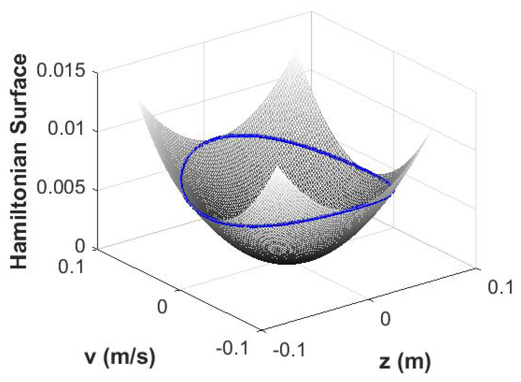
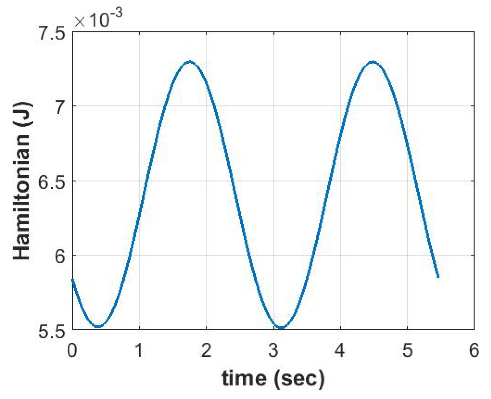
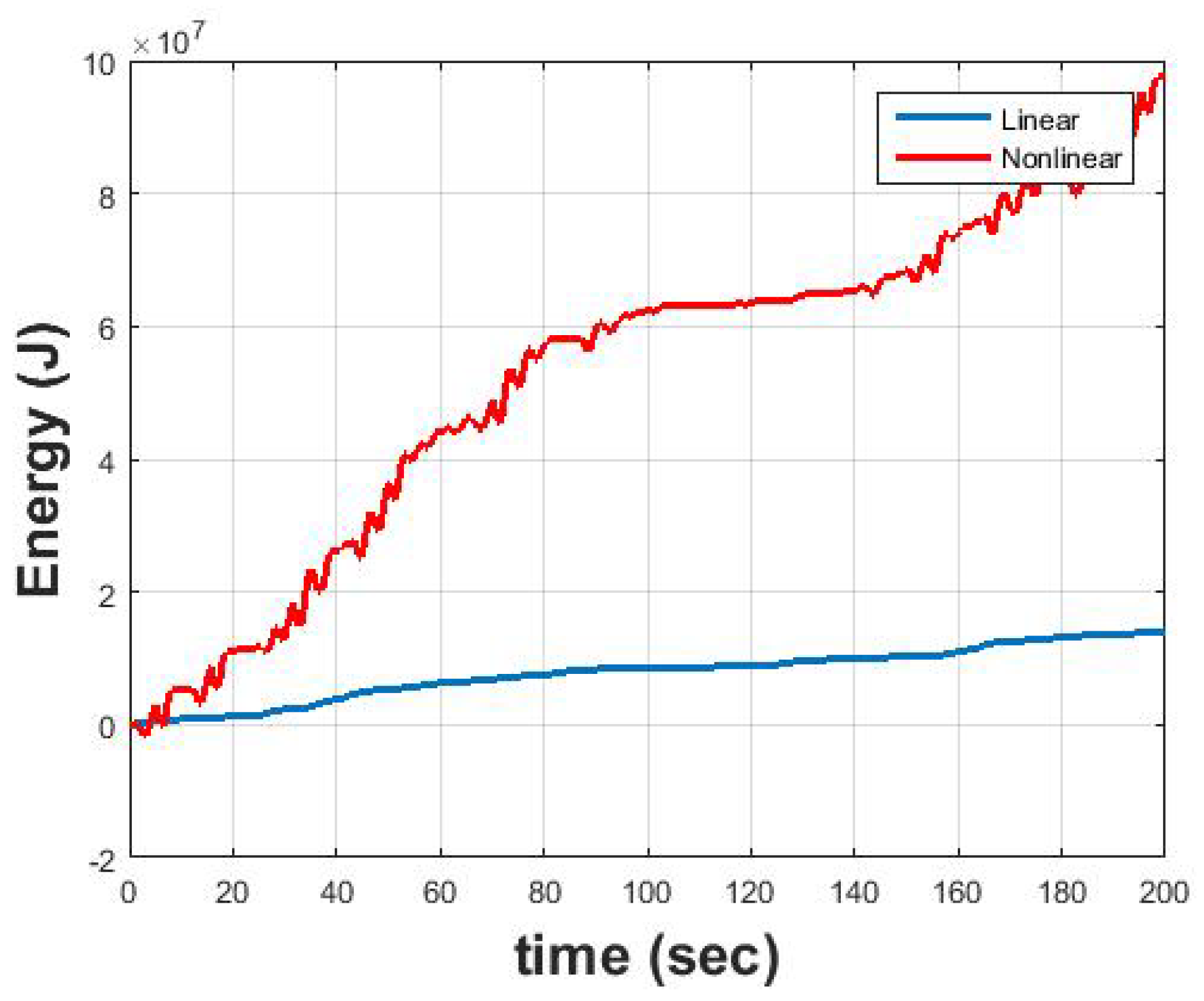
Finally, the power harvested by this buoy can be computed using Equation (3), where $u\left(t\right)=u_d\left(t\right)+{\sum }_{i=1}^{Nc}{\alpha }_{c_i}{z}^i$. One obtained solution for this case when $N_c=4$ is: ${\alpha }_1=-8048.03$, ${\alpha }_2=-6546.84$, ${\alpha }_3=8695.28$, ${\alpha }_4=7093.79$. Figure 3 shows the Hamiltonian surface and the WEC trajectory over one cycle. 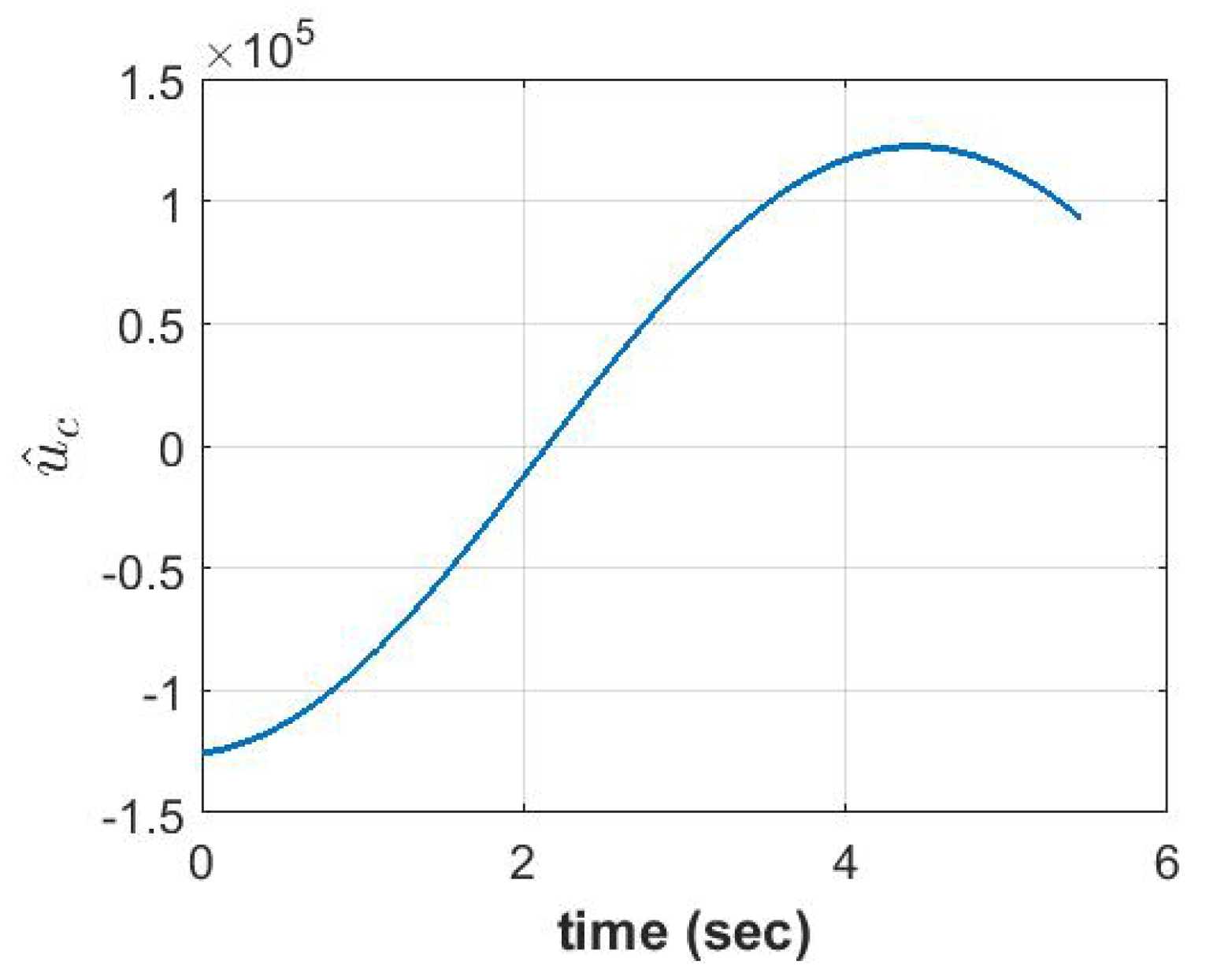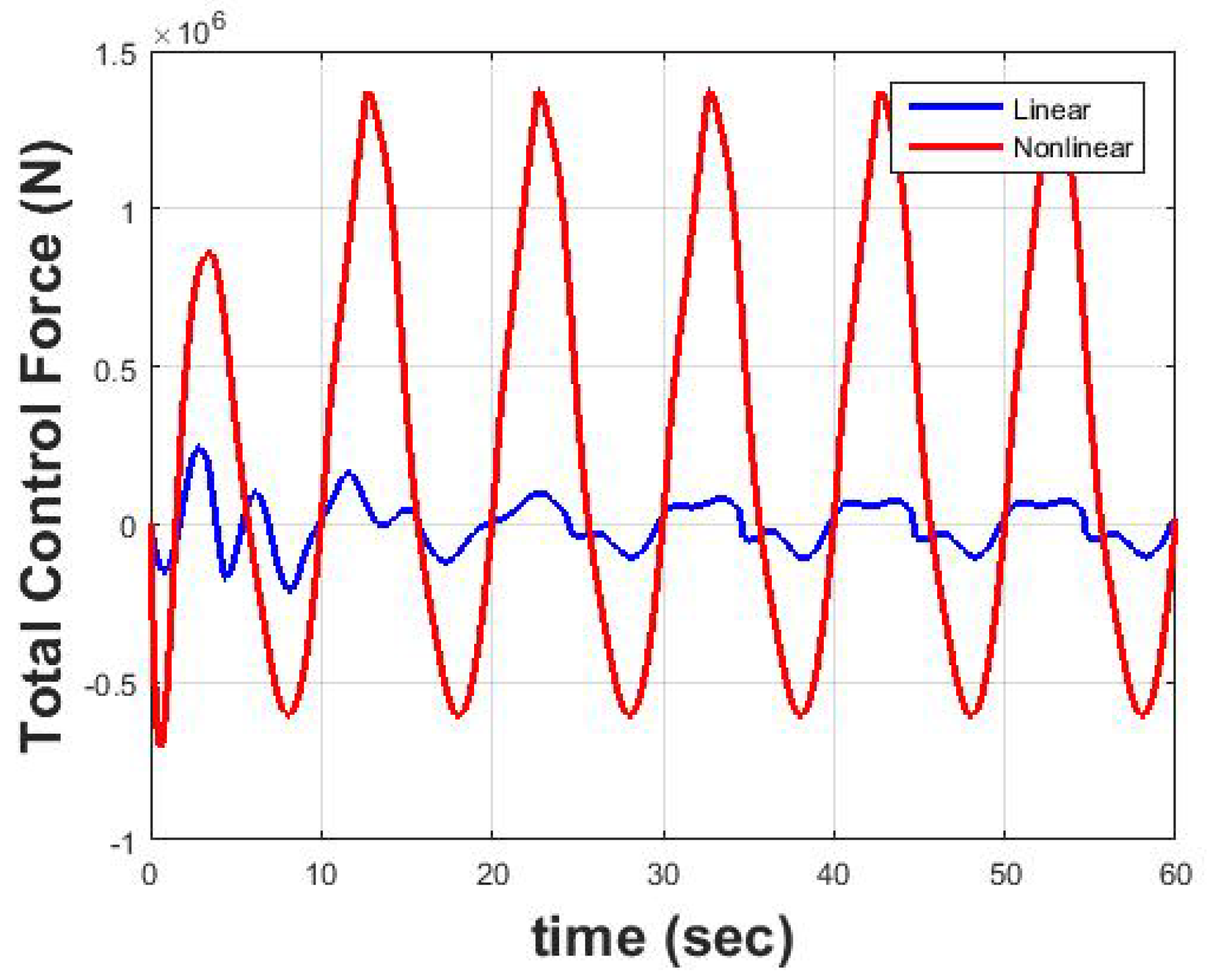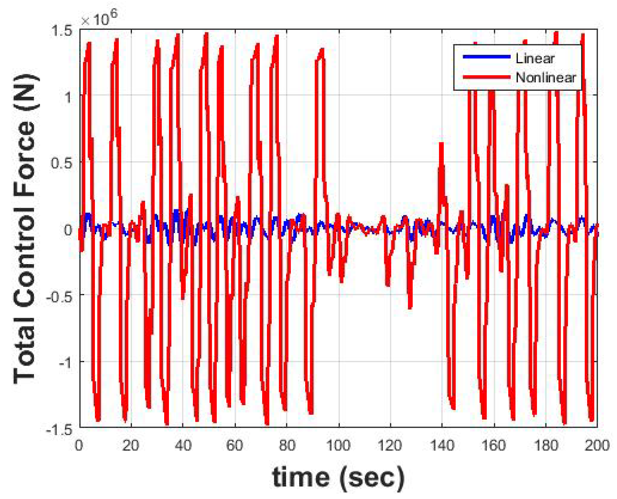The Hamiltonian changes over time and returns to its initial value after one cycle period, as shown in Figure 4. 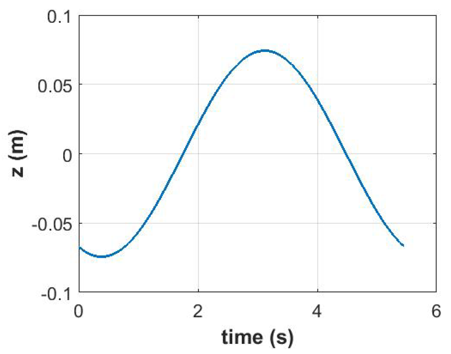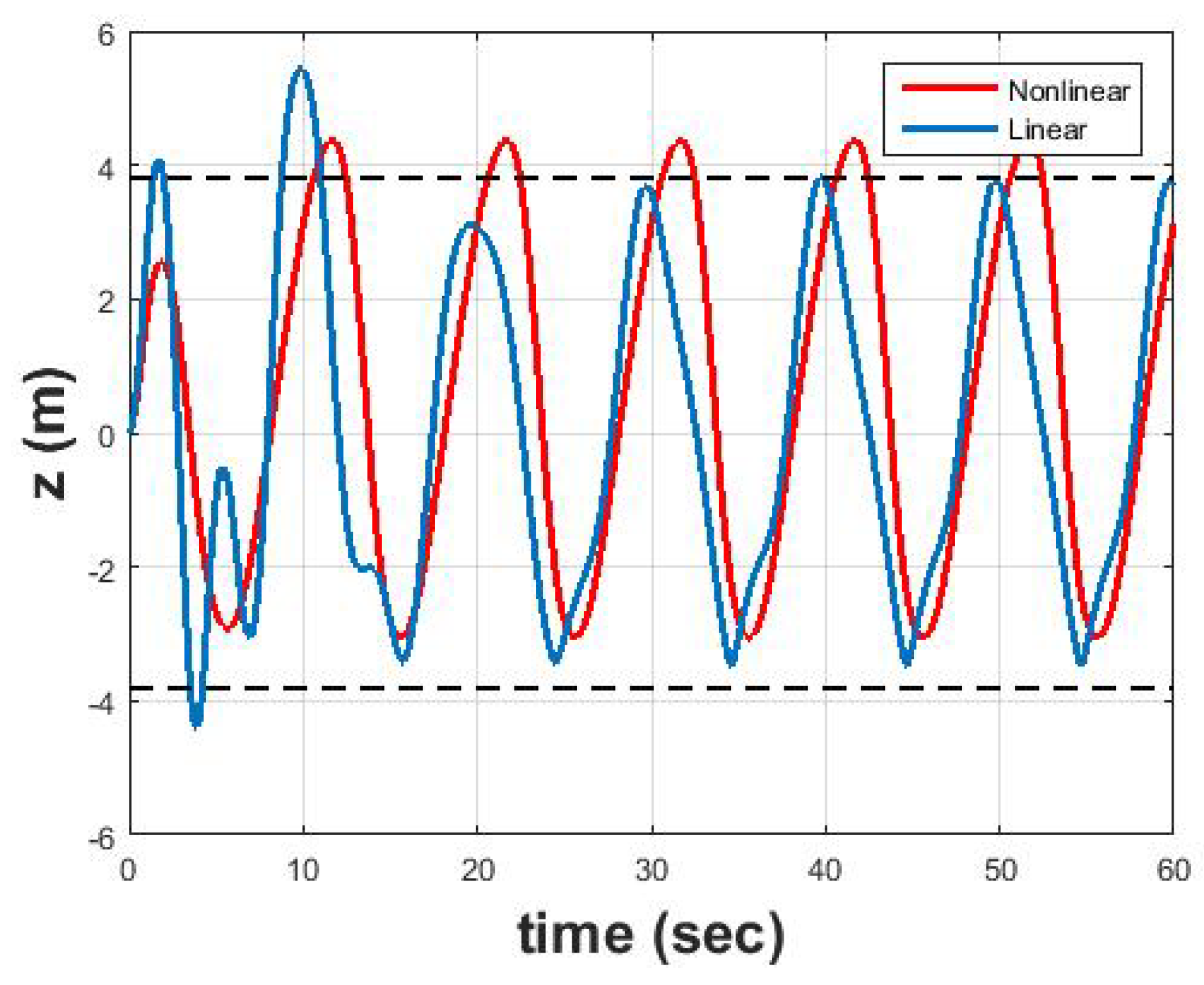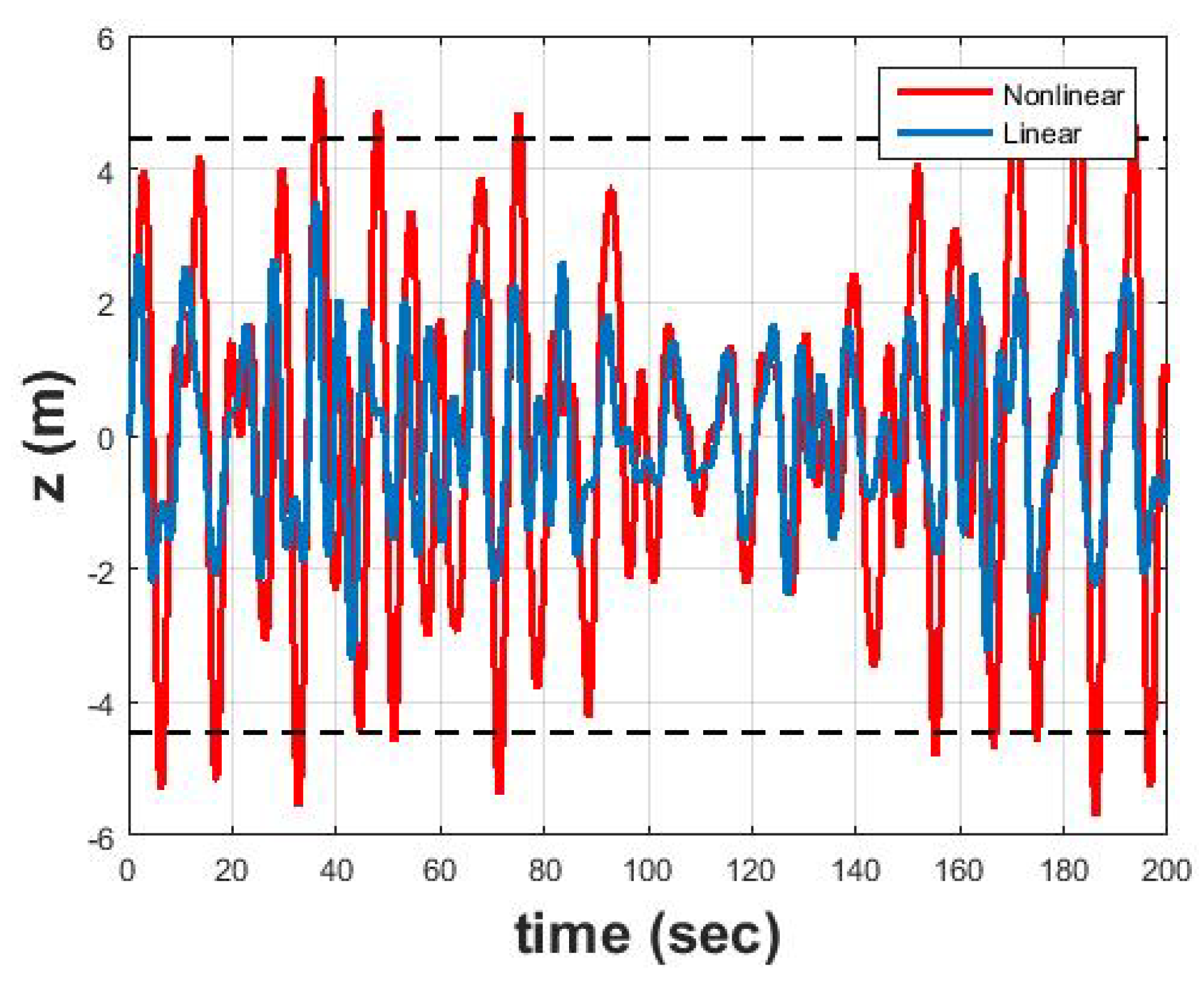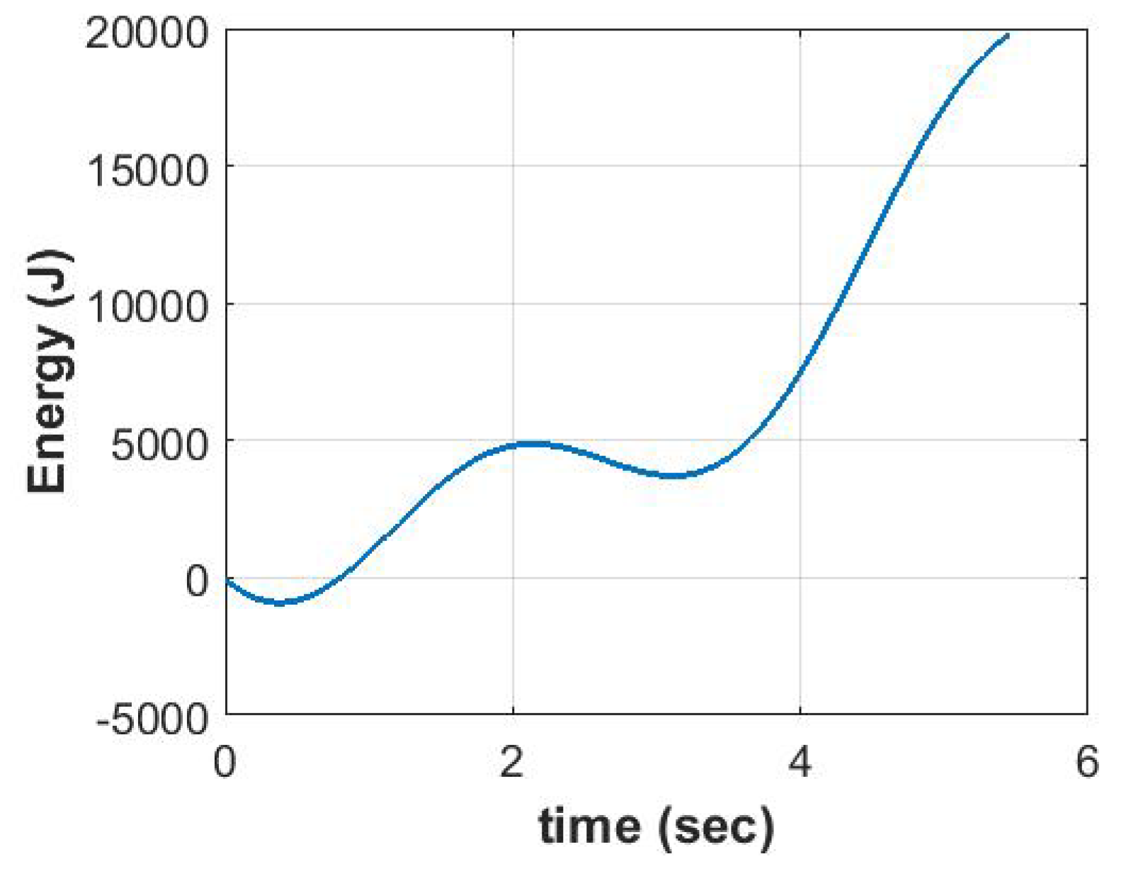The control force is shown in Figure 5, and the position of the buoy is shown in Figure 6. 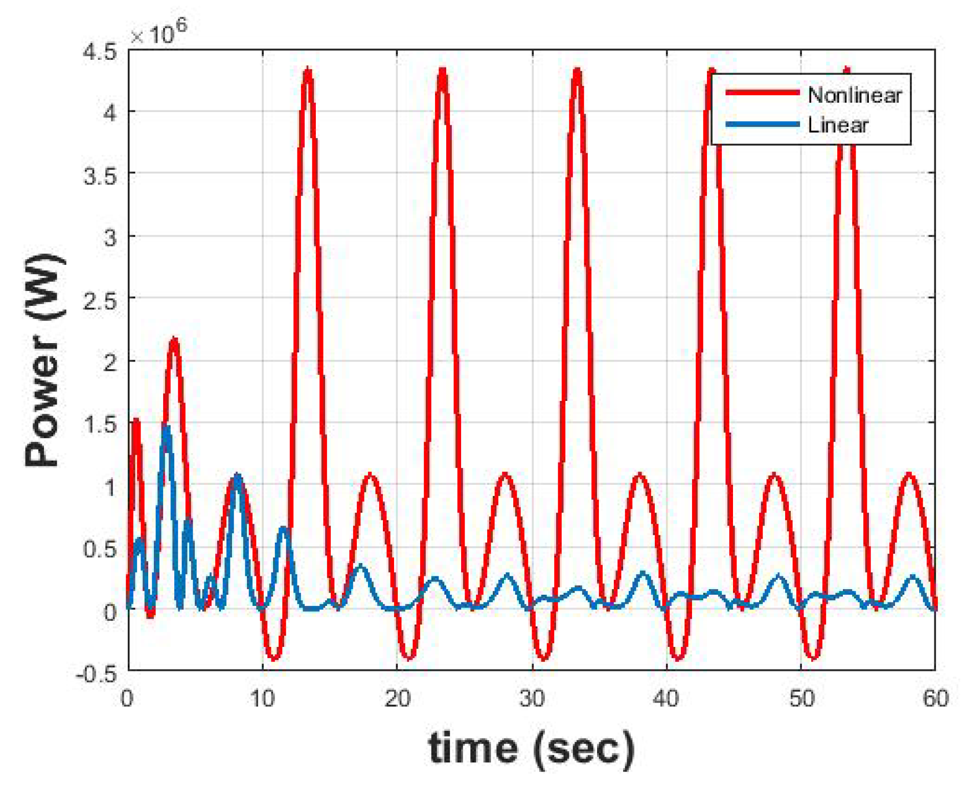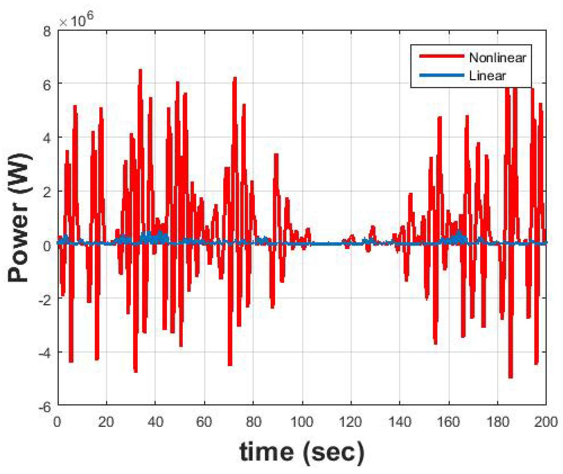The motion of the buoy is recurring, and the curve in Figure 6 repeats over time. The harvested energy in this case is plotted in Figure 7.

5. Case Study 2: Unprescribed Hamiltonian

In this section, the system is analyzed in regular and irregular waves. The Hamiltonian is not prescribed in this section; instead, the system of Equation (20) is simulated with the proposed control method (Equation (16)). The Hamiltonian of the system is calculated by numerical integration of Equation (29). Moreover, the performance of the proposed control method is compared to linear control. The focus of this section is to maximize the power extraction of the system and not achieving a system with $H_{cycle}=0$.

5.1. Regular Wave

In this section, two WEC control models are compared: the linear damping controller and nonlinear controller in the form of Equation (16). The wave is assumed regular, and the dynamic model of Equation (20) is assumed for both buoys.

Consider a cylindrical buoy of mass $1.76\times {10}^5$ kg. The buoy height and the limit $z_s$ are assumed $7.6$ m and $3.4$ m, respectively. The wave’s frequency is $0.62832$ rad/s, and its phase is $0.1$ rad. The linear stiffness force coefficient is $4.544915\times {10}^5$ kg/${\mathrm{s}}^2$; the radiation damping coefficient is 170 kg/s; and the reference amplitude of the excitation force is $1,319,900$ N. The first model uses only a linear control with a linear control force damping coefficient of $4\times {10}^4$ kg/s. The second model uses a nonlinear control force in which the number of control terms is selected as $N_c=4$ and $M_c=4$. The nonlinear control coefficients are ${\alpha }_c=[0,-61.6540,-49.0681,-99.7376]$ and ${\beta }_c=[4\times {10}^4,-5.3256,6.7505,-2.8242]$.

Simulations were conducted for 60 seconds for both cases, and the results are shown in Figure 8, Figure 9, Figure 10, Figure 11, Figure 12, Figure 13 and Figure 14. The extracted energy from the linear system is $9.592929\times {10}^6$ Joules, while the extracted energy from the nonlinear system is $5.924430\times {10}^7$ Joules, in 60 seconds, as shown in Figure 8. The nonlinear system produces about six times the energy harvested by the linear system. Figure 9 shows the power extracted by each system. The negative portions of the power curve are the reactive power portion that flows into the stiffness terms of the control. As expected, the linear system does not need any reactive power since the control is just a linear damping. The nonlinear system in this case needs reactive power, as shown in Figure 9. Note that the amount of reactive power dictates the size of the energy storage needed by the control system; and the control designs that do not need reactive power possess the advantage of lower cost and less complex systems compared to those control strategies that require energy storage. Figure 10 shows the displacement for both cases, where the dashed horizontal line represents the $z_s$ limit beyond which the buoy is considered either totally in the air or totally submerged. After an initial transition period, the displacements of both WECs have about the same amplitude and frequency; the same can be said about their velocities, as shown in Figure 11. Figure 12 shows the control force in which the nonlinear control requires about a $5.5$-times larger actuator in terms of the maximum control force. Figure 13 and Figure 14 show the Hamiltonian surface for the nonlinear and linear systems, respectively. Another way of examining the trajectory of states on the Hamiltonian surface is to plot the two-dimensional projection of the trajectory on the $z-\dot{z}$ plane; this is called the phase plot. Figure 15 shows the phase plot for both the linear and nonlinear control cases.

5.2. Irregular Waves

Consider the buoy described in Section 5.1. For the nonlinear control model, the radiation matrices for the cylindrical buoy, $A_r$, $B_r$, and $C_r$ were calculated using the added mass and damping coefficients obtained from the boundary element tool Nemoh.

Table 1. Radiation damping force parameters.

Matrix	Values
$A_r$	$\left[\begin{array}{cc}-0.97656& -0.98111\\ 1& 0\end{array}\right]$
$B_r$	$\left[\begin{array}{c}128\\ 0\end{array}\right]$
$C_r$	$\left[\begin{array}{c}216.07323\\ 0\end{array}\right]$

lists the numerical values of the radiation matrices. The excitation force ($F_{ex}$) is calculated as follows:

$$F_{ex}={\displaystyle \sum _{n=1}^N}{a}_n{F_e}_{n}exp(-i({\omega }_{n}t-{\varphi }_n))$$

(34)

where $a_n$ coefficients are the wave coefficients, ${F_e}_n$ coefficients are excitation force coefficients (calculated using Nemoh), ${\omega }_n$ variables are angular frequencies, and ${\varphi }_n$ describes the phase shift constants. In this case study, N is selected to be 260. A Bretschneider spectrum is assumed for the wave, while the frequency range is selected to be $\omega$ = [0.01:0.03698841:7], and the phase shifts are random numbers in $[-\pi ,\pi ]$. The significant wave height is selected to be $0.7$ m, and its peak period is assumed 10 s.

The nonlinear control parameters used in this case are listed in

Table 2. Control parameters selected in the case of WEC in an irregular wave.

Design Variable	Value
$N_c$	5
$M_c$	2
${\alpha }_c$	$[0,-7234.14,-7202.74,-825.04,5908.03]$
${\beta }_c$	$[-12836.26,-1221.05,0,0]$

. Simulation results are shown in Figure 16, Figure 17, Figure 18, Figure 19, Figure 20, Figure 21, Figure 22 and Figure 23. As can be seen in Figure 16, the total energy extracted using the linear control was $1.401074\times {10}^7$ Joules. The total energy extracted using the nonlinear control was $9.774873\times {10}^7$ Joules, which is about seven-times that of the linear control. The power extracted in both the linear and nonlinear models is shown in Figure 17; the nonlinear model requires much more reactive power compared to the linear model.

Figure 18 shows the displacement of the buoy over time for both models where the dashed horizontal line represents the $z_s$ limit. The motion of the nonlinear model is slightly higher than the linear model. However, the difference between the two systems in terms of buoy displacement is not significant. The same is true for the velocities for the two systems, as shown in Figure 19.

Figure 20 shows the total control force of both models. As shown, the nonlinear model requires significantly higher control force, meaning that it would need high performance actuators. The amount of required control force affects the mechanism and efficiency of the WEC, resulting in a trade-off between the extracted power and control force in designing WEC systems. Figure 21 is the phase plot for both linear and nonlinear models. As can be seen in Figure 21, the nonlinear system spans a larger area in the phase plane, enabling more power harvesting. Figure 23 shows the Hamiltonian surface for the linear system, and Figure 22 shows the Hamiltonian surface for the nonlinear system.

6. Conclusions

This paper presents the Hamiltonian surface approach, classically used in power flow analysis, in the analysis and design of control systems in wave energy conversion. A process of control design is demonstrated. This process guarantees a stable design for a control system, linear or nonlinear; but it does not guarantee the optimality of the solution. The case studies presented in this paper demonstrated the process for both regular and irregular wave spectra. It was shown that a nonlinear control can be designed to have a significant increase in the amount of harvested energy, given the availability of actuators that can provide higher force magnitudes, as well as the availability of storage systems and power take off units that can provide reactive power.