An Evaluation of the Wind and Wave Dynamics along the European Coasts

Abstract

The objective of this work is to analyze the wind and wave conditions along the coasts of the European seas. The emphasis is put on the mean and maximum values. The areas studied are characterized by intense maritime activities, including traffic, as well as various harbor and offshore operations. In the present study, 35 years of data (1983–2017) coming from the European Centre for Medium-Range Weather Forecasts (ECMWF) were processed, corresponding to 40 different geographical locations. Thus, these 40 reference points are defined for some of the most relevant offshore locations in the coastal environments targeted. As regards the data considered in the analysis, two different sets were used. The first corresponds to the wave model, while the second to the atmospheric model, both operated by ECMWF. Finally, it can be concluded that the proposed work provides a global perspective related to the average and maximum wind and wave conditions and to a further extent on the climate dynamics along the coasts of the European seas.

1. Introduction

The marine environments, either seas or oceans, can provide an economic advantage to any country regarding its level of development. Currently, we use seas and oceans not only for transportation, tourism, research, and fishing, but also for resource extraction. Furthermore, in the last few decades, we discovered the importance of the renewable resources to the detriment of the classical ones. Thus, wind and wave energy extraction comprises important projects not only in the developed countries, but also in the developing ones. However, due to the high cost of implementation and maintenance, these projects present also a high risk.

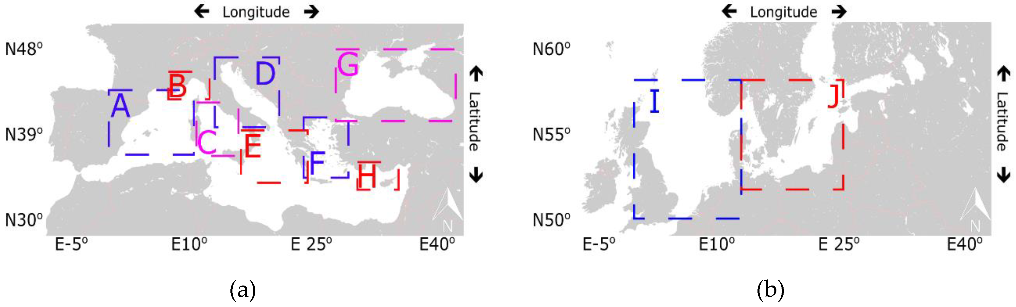
From this perspective, the objective of this work is to provide a comprehensive picture of the average and maximum wind and wave conditions along the European sea coasts. Thus, the paper presents the wind and wave conditions along the southern, southeastern, and northern costal environments of Europe. This includes the seas: Balearic, Ligurian, Tyrrhenian, Adriatic, Ionian, Aegean, Levantine, Black, North, and Baltic (Figure 1).

In the last few years, the demand for clean energy extraction started to spread all over the world, but above all in Europe [1], due to the increased air pollution context. Currently, most of the traditional methods for energy production (as for example those using oil, natural gas, or coal) face a major problem related to the need to reduce CO₂ emissions. The projections related to climate change indicate a direct relationship between the future dynamics of the climate and the CO₂ emissions. From this perspective, more and more international treaties impose prompt global warming actions to reduce the output of carbon dioxide to limit the levels of pollution. Thus, it is desired that the gap between the renewable resource extraction and the conventional methods be dramatically reduced [2,3,4,5,6], and therefore, many studies and coastal engineering applications have been focused on the energy potential of the offshore and nearshore marine environments [7,8,9,10,11]. Economically speaking, the marine areas have a significant role in the global financial mechanism. Besides the renewable energy extraction from waves [12,13,14,15,16,17,18,19,20,21,22], these areas are very competitive also as regards gross and passenger transportation.

Furthermore, the coastal environment of Europe is currently subjected to high navigation traffic and gross and passenger transportation and at the same time represents a proper environment for the energy extraction from renewable resources.

According to the European Commission, the total gross weight of goods handled at the ports of the European Union was estimated to be just above 3.8 billion tons in 2015, which means an increase of 13% from 2014. According to the same source, the total number of passengers was estimated as close to 395 million in 2015, an increase of 0.6% in relation with the previous year. However, over the last five years, the total number of passengers embarking and disembarking in the European Union ports has fallen by 7.0% [23].

From this perspective, it can be highlighted that the European marine environment is of great economic significance. However, at the same time, it can be a very dangerous one. Strong wind and waves that systematically occur can produce accidents with very serious consequences. In addition, high energy conditions may interrupt the extraction of renewable resources, as well as of the nearshore and harbor operations. Thus, the extreme conditions strongly affect the maritime navigation and can produce marine and coastal hazards that may have very high economic and ecologic consequences. From this perspective, a comprehensive picture of the average and maximum wind and wave conditions might be considered beneficial for maritime transportation, harbor, and offshore operations. To analyze and anticipate the behavior of the wind and wave conditions, climate studies have been performed. These studies imply using in situ measurements, which are limited to a specific location, reanalysis data coming from satellites that can provide data for extended geographical locations, or climatologic models [3,6]. This source can provide accurate information about the dynamics of the atmosphere or about the marine conditions. On the other hand, both means and maximum values of the wind and wave conditions are highly important for coastal and ocean engineering. These data are relevant for constructing not only nearshore structures, but also in relation to various offshore activities. In addition, these data can be a benefit to ship routing. Thus, this information is useful in the coastal management and maritime works, being a framework of reference in avoiding disasters by prevention and also for navigation and other marine engineering issues [24,25,26,27].

To this point, it can be mentioned that such a joint evaluation of the maximum wind and wave conditions, considering the analysis of 35 years of data and up to the present moment along the European sea coasts, might be considered of increasing interest in a proper evaluation of the trends corresponding to these environmental parameters and to a further extent from the perspective of the climate change assessment. In this connection, the objective of this work is to present a global perspective of the environmental matrix in the coastal environment of the European seas, focusing on the average and extreme wind and wave conditions. Thus, the main objective of the presented paper is to identify the most exposed locations in terms of hazards that may have high economic and ecological consequences, having also in attention the global picture of the environmental conditions in the European coastal environment.

2. Materials and Methods

2.1. The Target Areas

Figure 1 presents the zones considered in this study for analyzing the average and maximum conditions along the offshore of the European seas. More precisely, 10 different sea environments were taken into consideration, as presented before (

Table 1. The geographical locations and the characteristics of the considered reference points; the depths are relative to the mean sea level

Sea	Point	Lat.	Long.	Sea Depth (m)	Sea	Point	Lat.	Long.	Sea Depth (m)
Balearic	A1	40.075	1.000	100	Aegean	F2	36.850	26.925	110
	A2	41.700	3.200	127		F3	35.400	24.475	100
	A3	40.325	8.225	126		F4	36.990	23.025	130
	A4	39.400	2.225	118	Levantine	H1	36.250	29.270	106
	A5	37.750	−0.500	110		H2	35.375	33.570	116
Ligurian	B1	43.000	4.400	110		H3	34.660	32.440	126
	B2	43.850	9.850	115	Black	G1	43.700	30.000	130
Tyrrhenian	C1	42.625	10.400	128		G2	41.750	28.700	130
	C2	41.250	12.750	111		G3	42.150	34.000	107
	C3	39.375	15.975	123		G4	40.955	38.500	130
	C4	37.890	12.250	104		G5	44.225	38.575	100
	C5	39.400	9.725	121		G6	44.180	33.800	118
Adriatic	D1	43.230	14.750	106	North	I1	59.500	0.000	127
	D2	41.750	19.000	100		I2	57.950	5.200	118
	D3	40.000	18.500	110		I3	54.250	5.000	40
Ionian	E1	39.900	17.950	130		I4	54.000	1.225	40
	E2	39.000	20.600	130		I5	56.000	0.000	45
	E3	37.130	21.530	126	Baltic	J1	59.270	21.100	100
	E4	36.740	15.310	123		J2	56.570	19.900	130
Aegean	F1	39.625	25.300	123		J3	55.324	15.800	100

). Six of these zones (A, B, C, D, E, F, H, and G) are associated with the southern part of Europe (Figure 1a), another zone with the eastern part (G), and finally two others with the northern part of the continent (I and J) (Figure 1b). According to the methodology considered in the present work, as regards the choice for the selection of the reference sites studied, three aspects considered more significant were taken into consideration. The first is represented by the water depth. To be classified as offshore points, all sites had to be chosen for water depths of about 100 m, or greater. An exception is made for the North Sea, where depths higher than 100 m can be found only in the regions of Norway or Sweden. Thus, 3 points (I3, I4, and I5) have sea depths just over 40 m. Second, all points had to be located on the perimeter of a certain sea, and finally, the third aspect is that all points had to be located in the vicinity of the main European maritime ports and routes.

Figure 2a illustrates the geographical positions of reference points considered in the southern and eastern parts of Europe. Zone A is associated with the Balearic Sea. The Balearic Sea is located between the mainland of Spain (west) and the Balearic Islands (east) and south of the Ligurian Sea. The Ligurian Sea is bordered by France (west), Corsica (south), and Italy (north and east). In this area, five reference points have been selected (A1–A5). These points are located at an average depth of 116 m.

Zones B and C are associated with the Ligurian and Tyrrhenian seas, respectively. The Tyrrhenian Sea is enclosed by Sardinia (west), the Italian Peninsula (east), and Sicily (south). In these zones, seven reference points have been considered. Two of them are on the perimeter of the Ligurian Sea (B1–B2) at an average depth of 112 m, while the rest are located in the Tyrrhenian Sea (C1–C5) at an average depth of 117 m.

The Adriatic Sea is associated with Zone D. This sea is located between Italy (west), Slovenia, Croatia, Bosnia and Herzegovina, Montenegro, and Albania (east) and north of the Ionian Sea. In this area, three reference points have been selected (D1–D3). These sites are located at an average depth of 105 m.

Zones E, F, Gm and H are associated with the Ionian, Aegean, Black, and Levantine seas. The Ionian Sea is located south of the Adriatic Sea, between Greece (east) and Italy (west), and the Libyan Sea (south). The Aegean Sea is located between Turkey (east) and Greece (west). Zone G represents the Black Sea. The Black Sea is located between the Anatolian Peninsula and the southeastern part of Europe, between Bulgaria and Romania (west), Russia and Ukraine (north), Georgia (east), and Turkey (south) [7]. In this area, a total of six nearshore points were studied (G1–G6). These points are located at an average depth of 119 m. The Levantine Sea is located in fact at the eastern end of the Mediterranean Sea. This basin is bordered in the northwest by the Aegean Sea, in the north by Turkey, in the east by Syria, Lebanon, Israel, and the Gaza Strip, and in the south by Egypt and Libya [28]. In these zones, in total, eleven reference points correspond to these three zones. To analyze the maximum wind and wave conditions, four reference points have been selected in the area of Zone E (E1–E5), four in Zone F (F1–F6), and three others in Zone H (H1–H3). Regarding these three zones, the Zone E points are located at an average depth of 127 m, Zone F points at an average depth of 1157 m, while for Zone H, points correspond to an average depth of 116 m.

Figure 2b presents the geographical locations of the reference points selected for Zones I and J. The North Sea is located between Great Britain (west), Germany, the Netherlands, Belgium and France (south), and Finland and Denmark (east). The North Sea is in fact a marginal sea of the Atlantic Ocean. The Baltic Sea is bordered by Sweden (west and north), Finland, Estonia, Latvia, and Lithuania (east) and in the south by Poland and Germany. Zone I is associated with the North Sea, while Zone J with the Baltic Sea. In these geographical sectors, eight reference points were selected for analyzing the maximum wind and wave conditions. Five of them (I1–I5) belong to Zone I, and they have an average sea depth of 74 m, while the other three (J1–J3) have an average sea depth of 110 m.

2.2. The ECMWF Dataset

For the present study, information from the ERA-Interim database has been processed. ERA-Interim is a global reanalysis project developed and maintained by ECMWF (European Center for Medium-Range Weather Forecasts). This is an ongoing and complex project, 1979–present, that contains various parameters associated with the recent history of the atmosphere and of the marine environment [2,29,30].

In this study, the ERA-Interim data with a spatial resolution of 0.75° × 0.75° were processed. The time window considered in this paper was 35 years, 1 January 1983–31 December 2017, for two models. The first model is the atmospheric model, based on a spectral representation of the basic dynamical variables, a hybrid sigma-pressure vertical coordinate, and a semi-Lagrangian semi-implicit time stepping scheme [30]. The atmospheric model contains data for the zonal (u) and the meridional (v) wind velocities at 10-m height (U10). The wind velocity, corresponding to a certain location, resulted from interpolating the wind speed components between the grid points. In addition, the wind direction can also be determined using the same approach.

The second is the wave model, which is a component of the forecasting system and reflects the impact of the airflow on the ocean waves via the transfer of energy and momentum across the interface. The wave model incorporated in IFS (Integrated Forecast System) is based on the wave modelling (WAM) approach [30]. This model contains parameters such as the significant wave height of the combined wind-waves and swells (Hs), the mean wave direction (MWD), and the mean wave period (MWP). All the parameters presented are available for four intervals of six hours each (00-06-12-18 UTC) corresponding to each day [31].

WAM [32] is a wave model based on the spectrum concept, used to provide realistic estimates of the surface gravity waves for large-scale or global applications. Such a model is operated at ECMWF. Furthermore, compared to previous ECMWF reanalysis projects, such as the ERA40 [33], the ERA-Interim reanalysis project also assimilates the data via a 4D-Var method, using 11-km or 75-km spatial resolution.

The wave parameter analyzed in this work is the significant wave height of the combined wind sea and swell waves (Hs). For practical reasons, this will be named simply as significant wave height.

3. Results and Discussion

3.1. Wind Speed Analysis

Figure 3 illustrates an analysis of the wind speed at 10-m height corresponding to 35 years of data. The data presented in this figure were processed in terms of annual average ranges. Each box includes several key elements known as quartiles and whiskers. Those in the extremes are the upper and lower quartile and represent the 25th percentile of each data. The median value, red line, corresponds to the middle quartile and is equivalent to the 50th percentile of data. The whiskers are defined as 1.5-times the inter-quartile range. The data outside these elements are considered as outliers. However, they have also been included in the analysis.

In addition, Figure 3 includes the greatest value (excluding outliers) and the minimum (least value, excluding outliers) equivalent to the red crosses. The outliers are the observations that are numerically distant from the rest of the data. When analyzing a boxplot, the outliers are defined as data points that are located outside the whiskers. The mean values, black dots, were also processed. In some cases, the mean values were slightly higher than the median. This indicates a positive asymmetry and also that the outliers had a reduced influence on the mean values.

According to the data corresponding to Zones A, B, C, D, E, F, G, and H, we can notice that the annual averages intervals are narrower and have lower intensities. However, some extreme values are noticeable (extreme outlies) in the central region of the Mediterranean Sea. In these cases, these maximum values are defined as values that stand out in comparison with the associated dataset.

Corresponding to Figure 3, the wind is more intense in the northern area. Here, two zones were studied. Zone I, which is equivalent to the North Sea, and Zone J to the Baltic Sea. In these zones, the annual average intervals are wider. By comparing the mean values with the medians, a negative asymmetry can be found for Zone J. Here, the mean value is slightly smaller than the median.

A comparison of the U10 features in terms of maximum, 95th percentile, and average values is presented next. Thus, Figure 4 illustrates the values of the foregoing terms. In addition, Figure 4 highlights the upper four wind classes corresponding to the Beaufort scale. According to this scale, Class 12 represents wind greater than 32.7 m/s (hurricane), Class 11 wind speed in the range 28.5–32.6 m/s (violent storm), Class 10 the wind speed within the interval 24.5–28.4 m/s (full gale/storm), while class C9 corresponds to wind speed in the range 20.8–24.4 m/s (strong gale).

As can be seen in Figure 4, in quite a few points, the wind speed reaches the upper classes of the Beaufort scale. Class 9 is predominant. However, according to the data analyzed, in Zones I and J, the wind speed reaches extremes values. The predominant range is 24.5–28.4 m/s. The wind speed values above 32.7 m/s, equivalent to the hurricane level, can be found close to the west cost of the Scandinavian Peninsula. Another important aspect that is worth mentioning is represented by the differences between these three series (maximum value, 95th percentile, and average value). These differences imply that very high wind episodes can occur.

An additional more detailed analysis of the wind speeds’ annual averages was made by performing a comparison between the values for the winter and summer seasons. The winter season is considered in this work the six-month interval from October–March, while the summer season is the rest. This analysis is carried out for one location of each zone (selected considering the criterion that these are the locations with the highest average wind speed) and is presented in Figure 5. More precisely, the reference points A3, B1, C4, D3, E3, F1, G1, H2, I1, and J2 were selected. Even from a first glance, it can be noticed that during the winter season, the wind was considerably more significant. In most cases (D3, A3, B1, F1, C4, and G1), the differences between the winter and summer seasons as regards the wind speed average values were in the range 1.43–1.85 m/s. On the other hand, much higher differences for the average wind speed are noticed for the reference points I1 (2.77 m/s) and J2 (2.32 m/s). The smallest differences were recorded at points H2 (0.7 m/s) and E3 (0.56 m/s). The 95% confidence level of the linear trends and also the intervals of confidence are presented

Table 2. Linear trend confidence levels (CF) of the average annual wind speed, computed for 10 reference points (one of each zone) considered as the most representative. Results corresponding to the 35-year time interval 1983–2017. CF represents the 95.0% confidence level.

Point	A3			B3			C4			D3			E3
Interval	T	W	S	T	W	S	T	W	S	T	W	S	T	W	S
Mean	5.21	5.94	4.48	6.79	7.59	5.99	5.48	6.38	4.58	5.25	5.96	4.53	4.17	4.45	3.89
CF (95.0%)	0.07	0.13	0.08	0.10	0.16	0.12	0.07	0.14	0.07	0.08	0.11	0.10	0.05	0.10	0.07
Higher	5.28	6.07	4.56	6.89	7.75	6.11	5.55	6.52	4.65	5.33	6.07	4.63	4.23	4.55	3.96
Lower	5.14	5.81	4.40	6.69	7.44	5.87	5.40	6.24	4.51	5.16	5.85	4.44	4.12	4.36	3.83
Point	F1			G1			H2			I1			J2
Interval	T	W	S	T	W	S	T	W	S	T	W	S	T	W	S
Mean	6.16	6.98	5.35	5.92	6.85	4.99	3.86	4.22	3.51	8.49	9.88	7.11	7.18	6.03	6.03
CF (95.0%)	0.09	0.12	0.09	0.06	0.10	0.08	0.04	0.09	0.06	0.11	0.20	0.09	0.09	0.09	0.09
Higher	6.25	7.10	5.45	5.98	6.95	5.07	3.91	4.30	3.57	8.60	10.08	7.20	7.27	6.11	6.11
Lower	6.08	6.85	5.26	5.85	6.74	4.91	3.82	4.13	3.45	8.38	9.68	7.02	7.10	5.94	5.94

in correspondence with the linear trends presented in Figure 5. The resulting data show that according to the linear trends, the future estimates of the wind speed at 10-m height are expected to be in the range 0.04–0.16 m/s per decade. The climate change mechanism, being extremely complex and unpredictable, has a very likely impact on wind conditions. This assumption can be noticed in the linear trend.

Based on the annual, winter, and summer averages of the wind speed, the linear trends for the most representative points (one for each location) are presented in

Table 3. Linear trend (m/s per decade), values of the average annual wind speed, computed for 10 reference points (one of each zone) considered as the most representative. Results corresponding to the 35-year time interval 1983–2017. TLA represents the trend line for the annual averages, while TLW and TLS are the trend lines for the winter and summer seasons, respectively.

	A3	B1	C4	D3	E3	F1	G1	H2	I1	J2
Annual averages (TLA)	0.05	0.09	0.03	0.14	0.07	−0.07	−0.01	−0.02	−0.02	−0.07
Winter season (TLW)	0.06	0.11	0.05	0.10	0.11	−0.13	−0.08	−0.08	−0.05	−0.12
Summer season (TLS)	0.05	0.09	0.02	0.17	0.02	−0.01	0.06	0.05	0.00	−0.01

. At this point, it has to be highlighted that the linear trend values presented in this table are in line with those computed by other authors, as for example [34,35,36,37,38,39]. The data computed show slight increasing trends (ranging from 0.03–0.14 m/s per decade) for the reference points C4, A3, E3, B1, and D3, or decreasing trends for the points F1, J2, H2, I1, and G1 (ranging from −0.07–−0.01 m/s per decade).

3.2. Wave Analysis

An overview of the significant wave height, Hs, for all the ten zones considered is presented below. First, in Figure 6, the overall patterns of the significant wave height are presented. This figure provides a useful method to visualize the ranges and other features of the significant wave height for this large group of data. The data in this section were processed in terms of the yearly mean averages.

The differences between the northern region, the southern, and eastern regions respectively are obvious. Clearly, it can be noticed that in the North Sea region, the waves reached higher significant wave heights. Regarding the Baltic Sea, although the wind speed reached here considerable values, the annual means were comparable with those from the south and southeast.

According to the Douglas sea scale [40], there are 10 classes counting from zero. The most extreme in a reverse order are Class C9 with waves that are over 14 m (phenomenal waves), Class C8 with waves in the range 9–14 m (very high waves), Class C7 with waves in the range 6–9 m (high waves), Class C6 with waves in the range 4–6 m (very rough waves), etc.

Figure 7 presents a comparison for the significant wave height in terms of the maximum, 95th percentile, and average values. A notable aspect is that according to the 95th percentile analysis, the datasets are located below the class C6 line, except for the point I1. However, as Figure 7 shows, in some locations, about 5% of the waves are higher than 4 m. It can be also noticed that there are some places where the very high wave class is reached (C8). The maximum value line shows that significant wave heights have reached even 10 m.

Further on, Figure 8 presents the linear trend of the significant wave height estimated over the 35-year time interval considered. Thus, a comparison between the annual, winter, and summer season averages was conducted. As can be noticed from this figure, not just the wind speed was higher during the winter, but also the significant wave height followed a similar behavior. The results of this analysis show that the differences between the winter and summer averages are the range 0.29–0.7 m in about 90% of the cases (H2, E3, D3, B1, F1, G1, C4, A3, and J2). Nevertheless, a higher value for this difference results in the reference point I1 (1.25 m).

The slope of the trend line in meters per decade for the reference points A3, B1, C4, D3, E3, F1, G1, H2, I1, and J2 is presented in

Table 4. Linear trend (m per decade) values of the average significant wave height, computed for 10 reference points (one of each zone) considered as the most representative. Results corresponding to the 35-year time interval 1983–2017.

	A3	B1	C4	D3	E3	F1	G1	H2	I1	J2
Annual averages (TLA)	0.05	0.02	0.04	0.02	0.04	−0.01	0.01	0.01	0.02	−0.02
Winter season (TLW)	0.06	0.03	0.05	0.02	0.05	−0.02	−0.01	0.00	0.02	−0.05
Summer season (TLS)	0.04	0.02	0.03	0.01	0.03	0.00	0.03	0.02	0.03	0.00

. The trend line was processed for three distinctive intervals. The first one is related to the total year and indicates the annual averages (t.l.1), the second corresponds to the winter season (t.l.2), while the third to the summer (t.l.3). The results show a slightly increasing trend (ranging from 0.01–0.04 m per decade) for about 80% of the reference points. More precisely, this trend is valid for the points G1, H2, B1, D3, I1, C4, E3, and A5. On the other hand, the results show also slightly decreasing trends for the reference points F1 and J2. It can be also noticed that the winter and the summer seasons do not show the same trends. An interesting situation as been relates the reference points G1, H2, and I1. Thus, even if wind speeds had a slightly decreasing trend (Table 2), the significant wave heights were increasing.

Table 5. Linear trend confidence levels of the average significant wave height, computed for 10 reference points (one of each zone) considered as the most representative. Results corresponding to the 35-year time interval 1983–2017. CF represents the 95.0% confidence level.

Point	A3			B3			C4			D3			E3
Interval	T	W	S	T	W	S	T	W	S	T	W	S	T	W	S
Mean	1.10	1.37	0.84	0.85	1.05	0.66	0.99	1.25	0.73	0.58	0.74	0.43	0.61	0.75	0.47
CF (95.0%)	0.03	0.05	0.03	0.02	0.03	0.02	0.03	0.05	0.02	0.01	0.02	0.01	0.02	0.03	0.02
Higher	1.13	1.42	0.86	0.87	1.08	0.67	1.01	1.29	0.75	0.60	0.76	0.44	0.63	0.79	0.48
Lower	1.07	1.32	0.81	0.83	1.02	0.64	0.96	1.20	0.70	0.57	0.72	0.41	0.59	0.72	0.45
Point	F1			G1			H2			I1			J2
Interval	T	W	S	T	W	S	T	W	S	T	W	S	T	W	S
Mean	0.79	1.00	0.58	0.90	1.14	0.67	0.46	0.57	0.36	2.27	2.90	1.64	1.21	1.55	0.86
CF (95.0%)	0.02	0.03	0.02	0.02	0.03	0.02	0.01	0.02	0.01	0.04	0.07	0.03	0.03	0.05	0.02
Higher	0.81	1.02	0.60	0.92	1.17	0.69	0.47	0.59	0.37	2.31	2.96	1.67	1.23	1.60	0.88
Lower	0.77	0.97	0.57	0.89	1.11	0.65	0.46	0.56	0.35	2.23	2.83	1.61	1.18	1.51	0.84

provides the linear trend 95% confidence level, while the higher and lower limits with respect to the trend lines are presented in Figure 8. Therefore, the linear trends illustrated in Figure 8 and the data from Table 5, estimate that the future significant wave heights can increase or decrease in the range 0.01–0.07 m per decade.

At this point, it can be mentioned that the resulting data are in correspondence with the analysis conducted by some other authors, as for example [40,41,42]. The mechanism of the wave formation is extremely complex due to the high number of variables. The wind speed is only one of them, but the most important one. However, the increase in wind speed does not always mean the increase of the of local significant wave height. This can be seen by comparing the linear trend data for the wind speed and significant wave height.

3.3. Maximum Conditions Analysis

This section contains a detailed analysis of the extreme marine conditions along the European coastlines. Two parameters coming from ECMWF ERA-Interim were studied. These are the significant wave height (Hs) and the wind speed reported to 10-m height (U10) above the sea level. The target time interval consists of 35 years (1 January 1983–31 December 2017). The data in this section were processed for the total time interval. The histograms from Figure 9 present the frequency of distribution for the paraFiguremeters Hs and U10. Furthermore, the normal distribution corresponding to each parameter has been represented, and it can be noticed that the distribution of the wind speed follows very well the Gaussian shape. On the other hand, according to [35], as regards the significant wave height, this appears to be better described by the Weibull distribution. In this analysis, the 10 most representative locations, one from each zone, were considered and studied. From Figure 9 and

Table 6. Hs and U10 statistics of the most representative points. The results are available for the 35-year time interval 1983–2017.

		A3	B1	C4	D3	E3	F1	G1	H2	I1	J2
Hs	standard deviation	0.89	0.65	0.74	0.48	0.44	0.65	0.64	0.34	1.22	0.85
	mean	1.10	0.85	0.99	0.58	0.61	0.79	0.90	0.46	2.27	1.21
	median	0.80	0.60	0.80	0.40	0.50	0.60	0.70	0.41	2.00	1.00
	mode	0.40	0.20	0.50	0.30	0.20	0.20	0.50	0.40	1.40	0.50
	skewness	1.66	1.38	1.73	1.77	1.69	1.66	1.83	2.21	1.23	1.38
	kurtosis	3.40	1.94	4.14	4.08	3.85	3.53	4.77	7.17	2.01	2.36
U10	standard deviation	3.00	3.97	3.00	2.94	2.19	3.49	2.94	2.05	4.02	3.36
	mean	5.21	6.79	5.48	5.25	4.17	6.16	5.92	3.86	8.49	7.19
	median	4.70	6.09	4.98	4.85	3.87	5.67	5.60	3.60	8.14	6.88
	mode	1.23	1.97	4.50	2.69	3.83	5.17	4.16	3.09	3.80	5.33
	skewness	0.85	0.57	0.77	0.74	0.75	0.63	0.56	0.95	0.46	0.47
	kurtosis	0.60	−0.43	0.40	0.38	0.55	−0.04	0.10	1.41	0.00	−0.01

, several key aspects can be noticed. The skewness indicates the degree of symmetry in the variable distribution (Equation (1)). The skewness is indicated also because the average values are higher than the medians and modes, and the medians are higher than the modes. Thus, it results in a positively-skewed distribution (positively skewness) or skewed to the right (skewness > 0). The other key aspect is represented by the kurtosis analysis (Equation (2)). This analysis is a measure of whether the data are light-tailed relative to a normal distribution or are heavy-tailed. According to the information from Table 1, the data for the Hs parameter were leptokurtic (peaks sharply with fat tails, equivalent to the kurtosis coefficient >0). Regarding the U10 parameter, the data were leptokurtic or mesokurtic (normal distribution equivalent with kurtosis coefficient = 0) or platykurtic (flattened, equivalent with kurtosis coefficient <0).

$$s=\frac{E{\left(x-\mu \right)}^3}{{\sigma }^3}$$

(1)

$$k=\frac{E{\left(x-\mu \right)}^4}{{\sigma }^4}$$

(2)

where µ represents the mean value, σ is the standard deviation, and E(x) represents the expected value of the quantity x.

A classification of the maximum wind and wave conditions is presented next. This analysis is based on the Beaufort scale. This is an empirical method to classify the sea conditions in relation to the wind speed. According to the Beaufort scale, there are 13 classes (0–12, 12 being the highest of intensity). To measure the extreme conditions in the studied area, only four classes were used (C9 strong/severe gale, C10 storm/whole gale, C11 violent storm, and C12 hurricane force).

The Hs parameter inferior limit for the C9 class is 7 m, while for U10, it is 20.8 m/s.

Table 7. Maximum wind and wave conditions according to the Beaufort scale for the Mediterranean, Black, and Baltic seas.

Reference Point	Year	Month	Day	Interval	Hs (m)	Wave Class	U10 (m/s)	Wind Class
Point A3	1987	1	11	18	7	C9	18.5	no storm class
	1999	12	28	12	7.3	C9	17.4	no storm class
Point B1	1996	2	8	6	3.8	no storm class	21.1	C9
	1996	2	8	12	4.8	no storm class	21.2	C9
	2012	10	28	6	4.5	no storm class	21.5	C9
	2012	10	28	12	4.3	no storm class	20.9	C9
Point F1	2004	1	22	12	5.4	no storm class	21.5	C9
Point J2	1984	1	13	18	5.4	no storm class	22.8	C9
	1990	12	29	12	3.8	no storm class	21.3	C9
	1993	1	14	6	4.9	no storm class	22.3	C9
	1993	2	17	0	3.4	no storm class	25.6	C10
	1993	2	19	0	3.1	no storm class	21.3	C9
	1999	12	17	18	5.6	no storm class	22.0	C9
	2000	3	3	12	4.6	no storm class	21.6	C9
	2002	2	22	18	6	no storm class	21.2	C9
	2005	1	9	0	7.5	C9	22.3	C9
	2005	1	9	6	7.3	C9	19.8	no storm class
	2011	12	9	6	3.9	no storm class	26.3	C10
	2015	1	11	0	5.5	no storm class	20.9	C9

and

Table 8. Maximum wind and wave conditions according to the Beaufort scale for the North Sea.

Point	Wave Class	Hs Mean (m)	Wind Class	U10 Mean (m/s)	Occurrences
I1	C9	7.5	no storm class	18.8	138
	C9	7.8	C9	22.0	82
	C9	7.8	C10	25.3	6
	C9	8.4	C11	29.4	1
	C9	7.0	C12	35.2	1

present an overview of the wind and wave extreme conditions along the European coastline. According to the resulting data during the 35-year interval, in the Mediterranean and the Black seas, few events were noticed that can be classified as extreme. As can be noticed in Table 5, in the Black Sea in relation to the data for the Mediterranean Sea, neither wave nor wind conditions were met in order to classify the event to be an extreme one.

In addition, these events never exceeded the duration of one day. Regarding now the northern part of Europe, the North and Baltic seas, things are different. In this region, the significant wave height never exceeded the superior limit of the C9 class. This is 24.4 m. However, it can be noticed that in the North Sea, 228 potential dangerous events occurred, during which the U10 parameter had values in the range 18.8–35.2 m/s. Although the wind reached high intensity, the Hs parameter never crossed the upper limit of the C9 class. This is 10 m.

The ERA-Interim dataset contains information about the zonal and meridional velocities. This information is needed in order to analyze the main wind directions. More precisely, this is the directions from which the wind is blowing. The wind roses illustrated in Figure 10 correspond to the two seasons (winter and summer, lasting six months each). The dominant directions and also the predominant wind speed range corresponding to all the ten locations are presented in Figure 10. In this figure, the range of the wind speed was divided into 12 intervals. At first sight, the data show that the most frequent values of the wind speeds were in the interval 0–12 m/s. However, it has to be noticed that for the points located in the northern part of Europe (I1 and J2), this observation is not valid. Thus, in these locations, the wind roses show that the most frequent values of the wind speeds were in the seventh interval (18 ≤ U10 ≤ 21 m/s).

The wind roses presented in Figure 10 correspond also to the two seasons considered, each of six months. By analyzing the data, it can be noticed that the most significant difference between these seasons was that in winter, the wind was more intense, while the direction of blowing was spread or shifted.

4. Conclusions

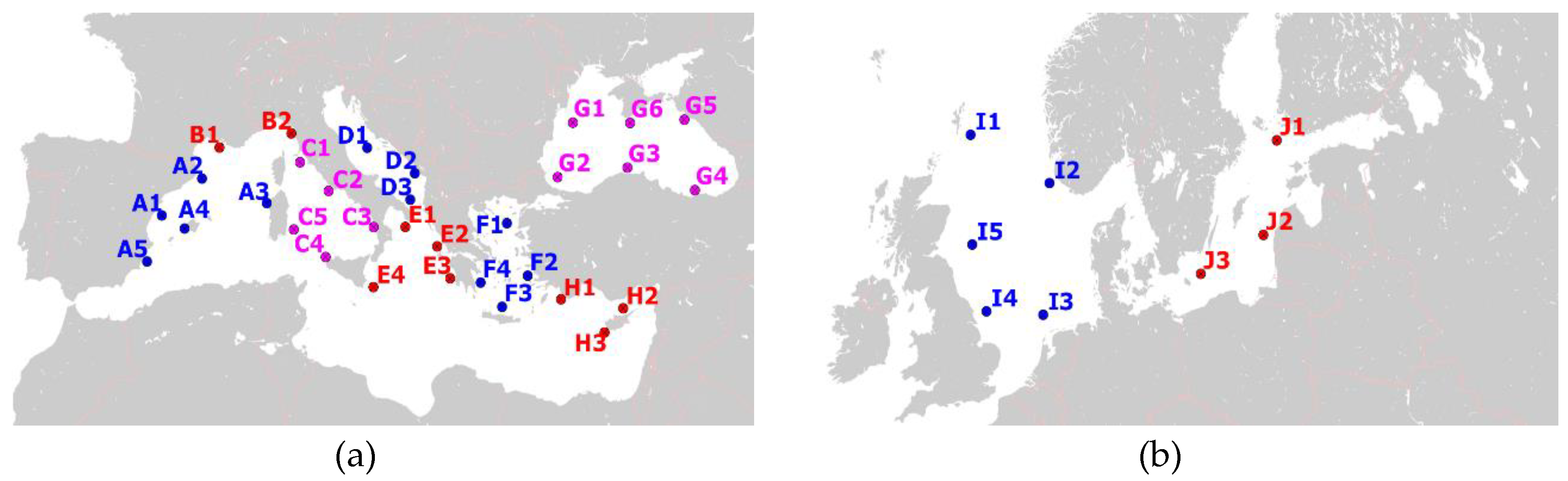
In this work, the offshore conditions in the coastal environment of Europe were assessed in order to provide an analysis of the average and maximum wind and wave conditions. Some of the environmental parameters coming from the ECMWF ERA-Interim dataset were studied for the 35-year time interval (1 January 1983–31 December 2017). More specifically, the significant wave height (Hs) and the wind speed at 10-m height above the sea level (U10) were processed. The target seas were the Balearic, Ligurian, Tyrrhenian, Adriatic, Ionian, Aegean, Levantine, Black, North, and Baltic seas. The data for this study were processed corresponding to 40 different geographical locations.

From this perspective, the present study provides a global perspective related to the average and maximum wind and wave conditions and to a further extent on the climate dynamics along the coasts of the European seas. At this point, it has to be highlighted that several separate studies have been previously performed for each sea environment considered, and the results are consistent with those coming from the present work. Thus, in the Mediterranean Sea, the wind energy potential was evaluated in [36], while the wave conditions in [5]. Along the coasts of the Black Sea, the synergy between wind and wave power was analyzed and interesting results presented in [37,38]. Finally, the results of a 41-year hindcast in the Baltic Sea were presented in [39].

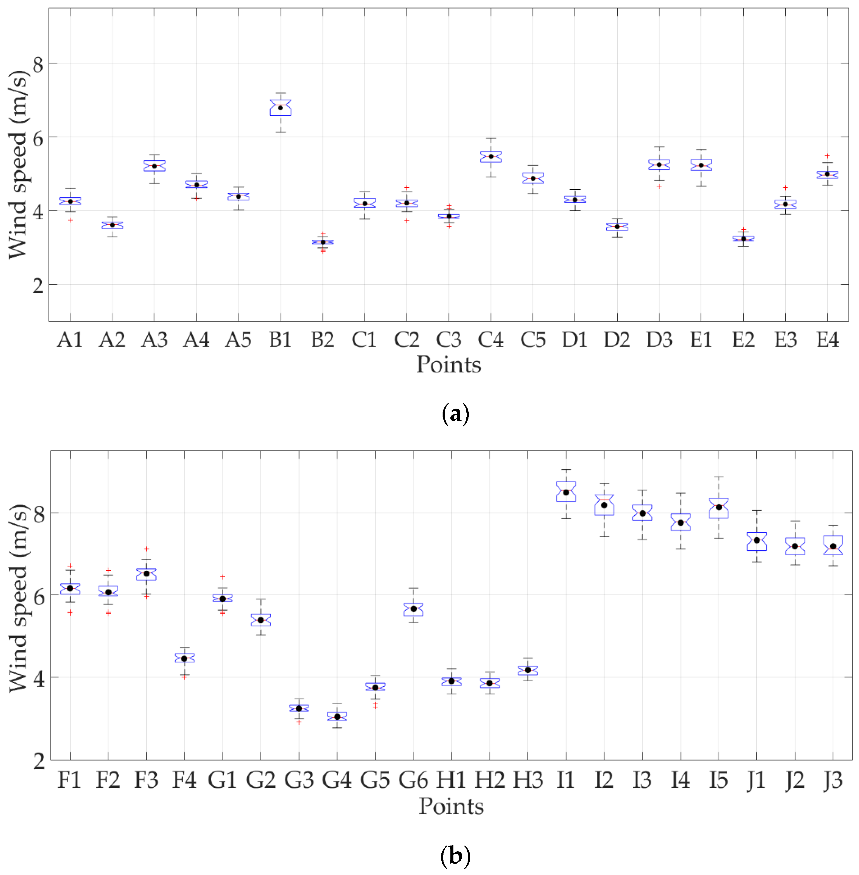
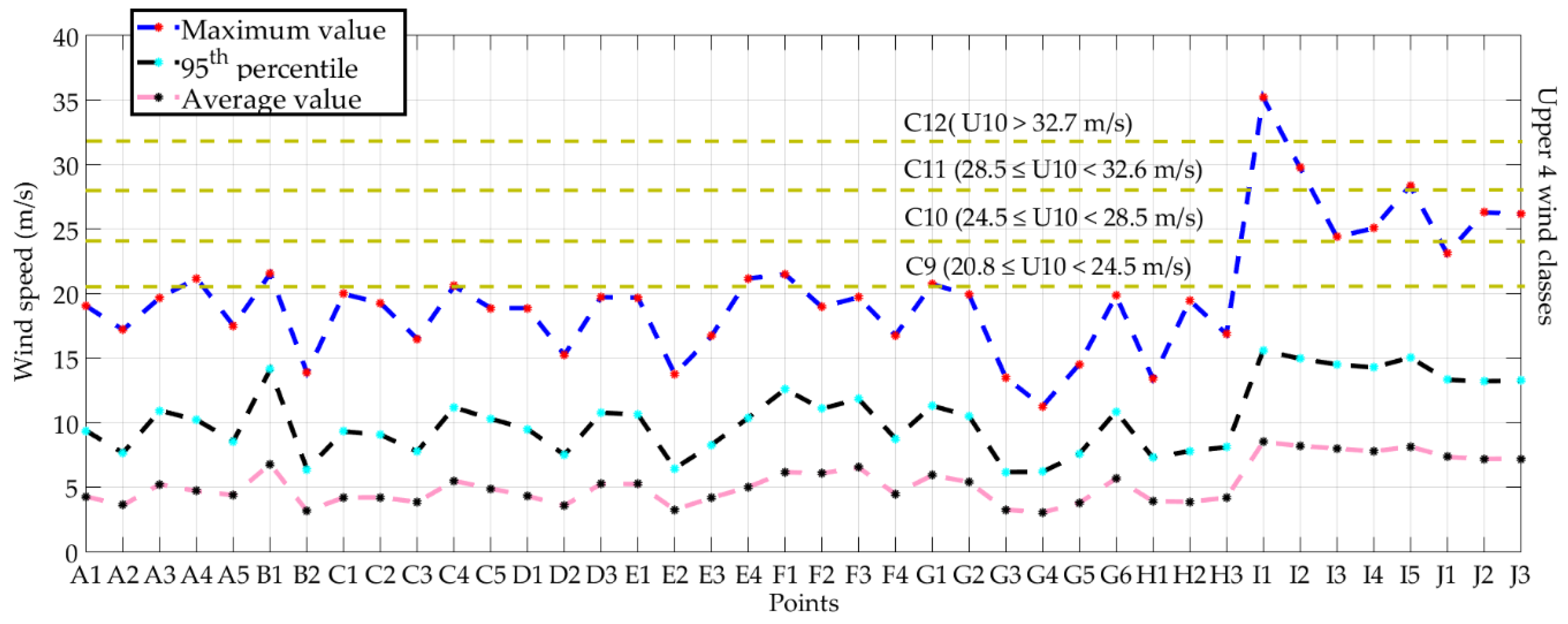
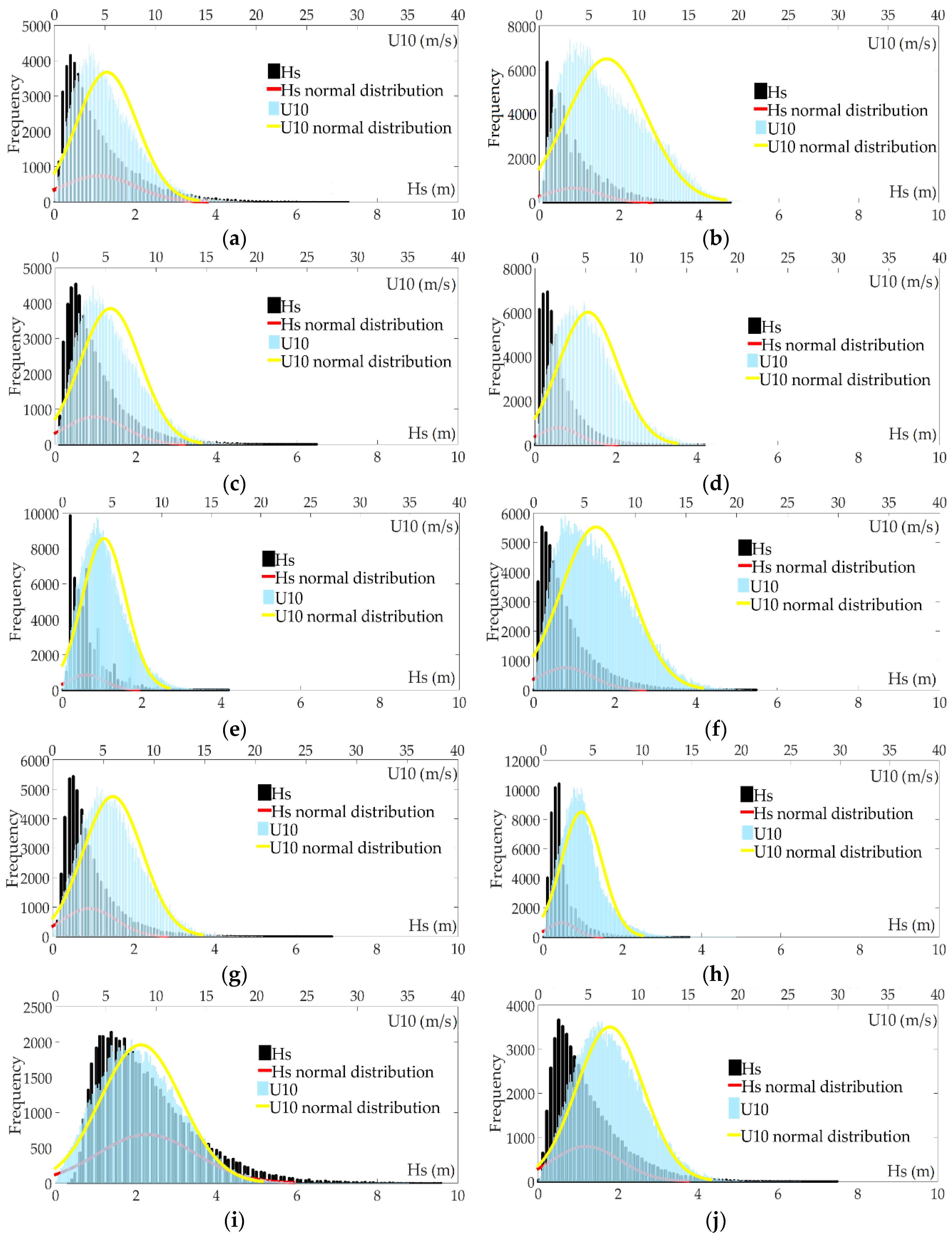
As discussed in this work, the wind intensity is considerably higher in the northern part of Europe, especially in the North Sea region. According to the results, 5% of the wind speeds for the point I1 (from the North Sea) are in the range 15–35.2 m/s. Extremely high values up to 30 m/s can be found not only in the North Sea, but also in the Baltic Sea.

These episodes can affect not only ship transportation, but also renewable energy extraction. The cut-out wind speed for many of the offshore wind turbines is 25 m/s. This implies that in such regions, operation interruptions or even damages can occur.

The southern and the eastern marine environments of Europe seem to be safer in terms of the wind intensity. In these regions, the wind speed is just over 20 m/s for 12.5% of the points studied.

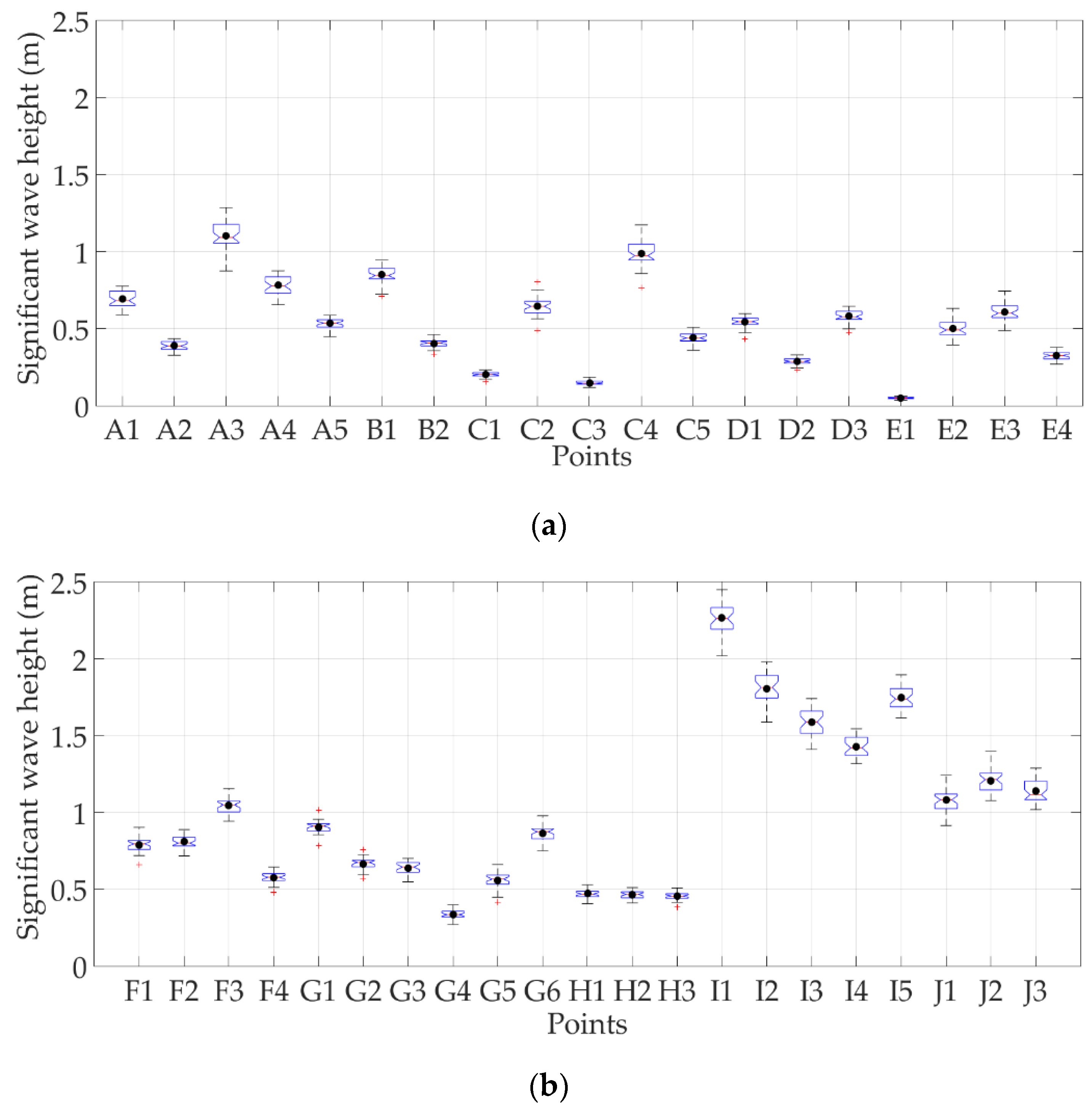
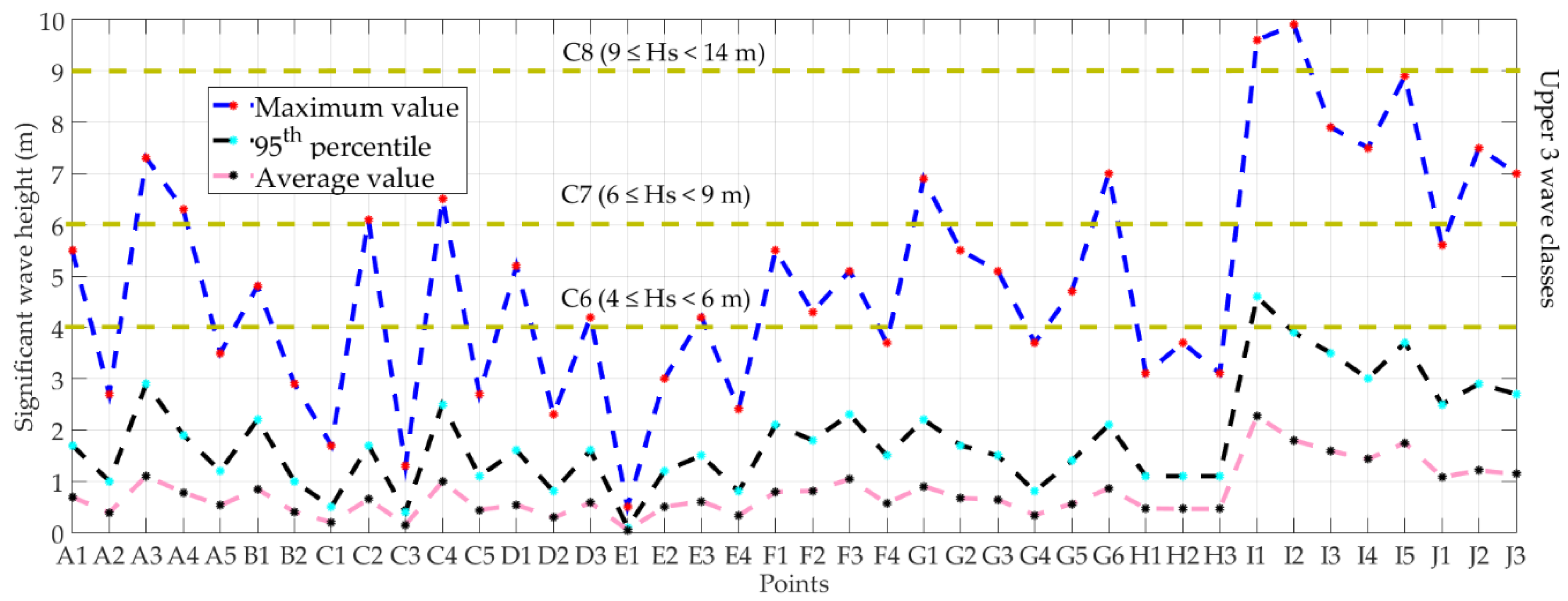
Furthermore, by performing a comparison between the wave and the wind data, an association can be noticed regarding the zones with higher intensity. The parameter Hs reaches higher values in the northern part of Europe. Here, the maximum values are in the range 5.5–10 m.

Regarding the southern and the eastern part of Europe, the picture is quite different. There are points where Hs reaches values up to 7.3 m. On the other hand, there are also points were the maximum significant wave height never reached even 1 m.

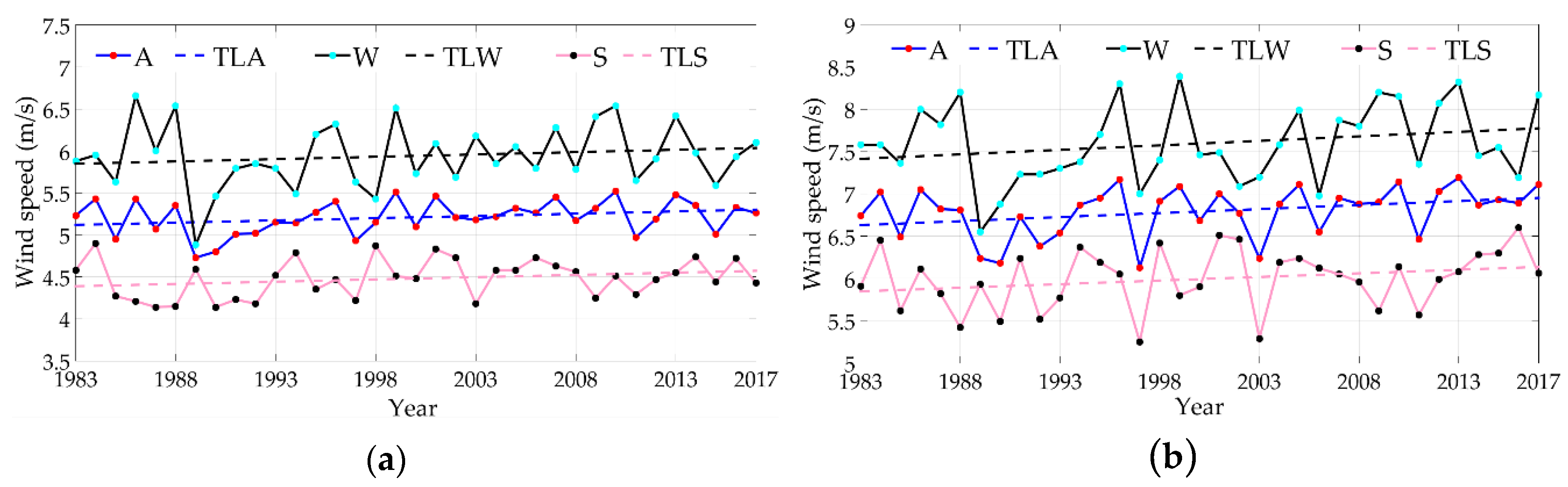
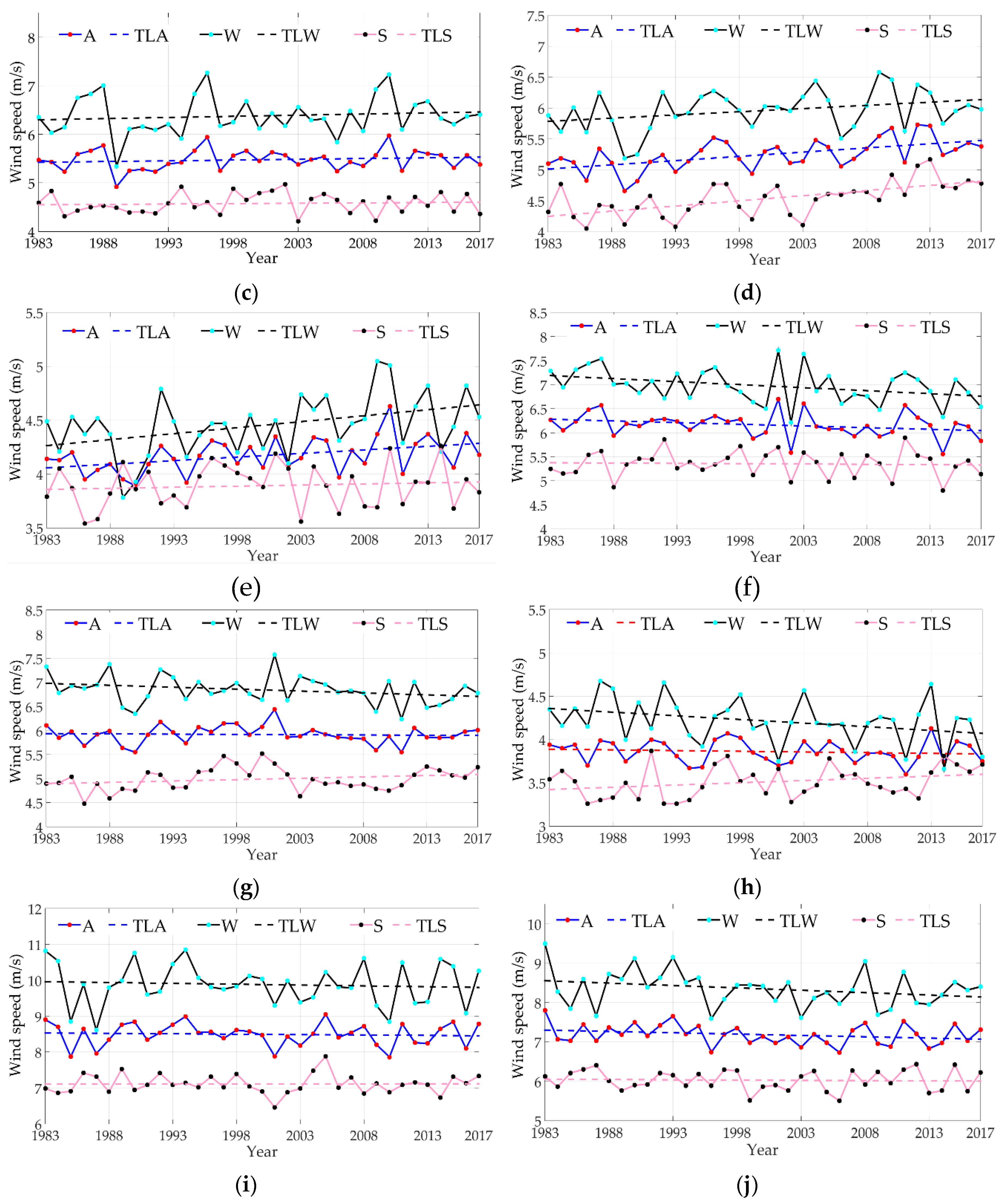
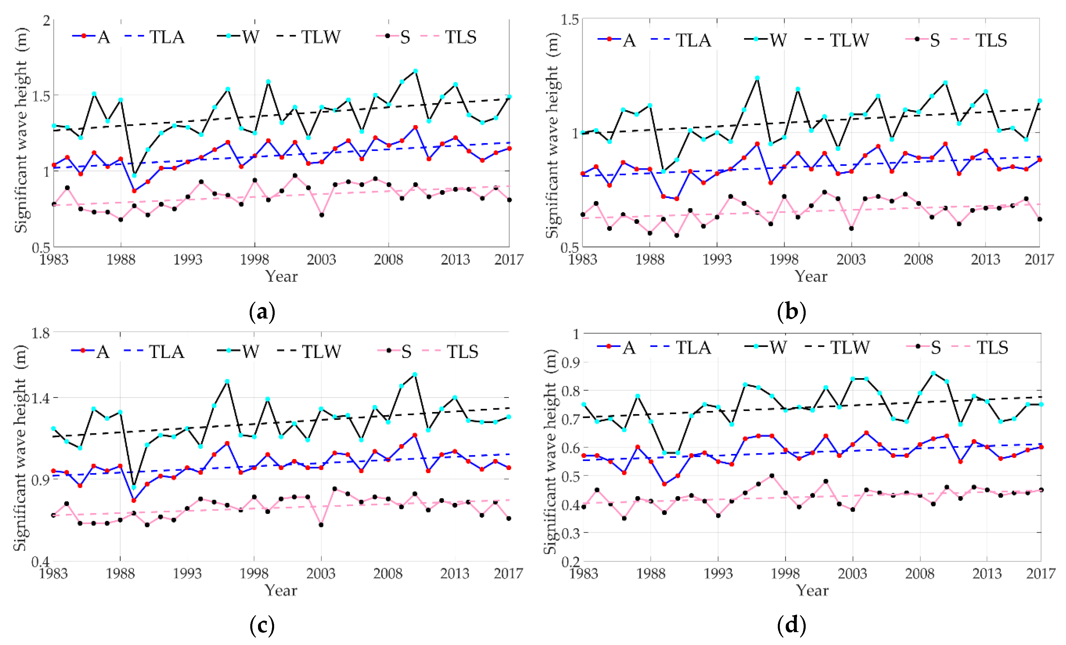
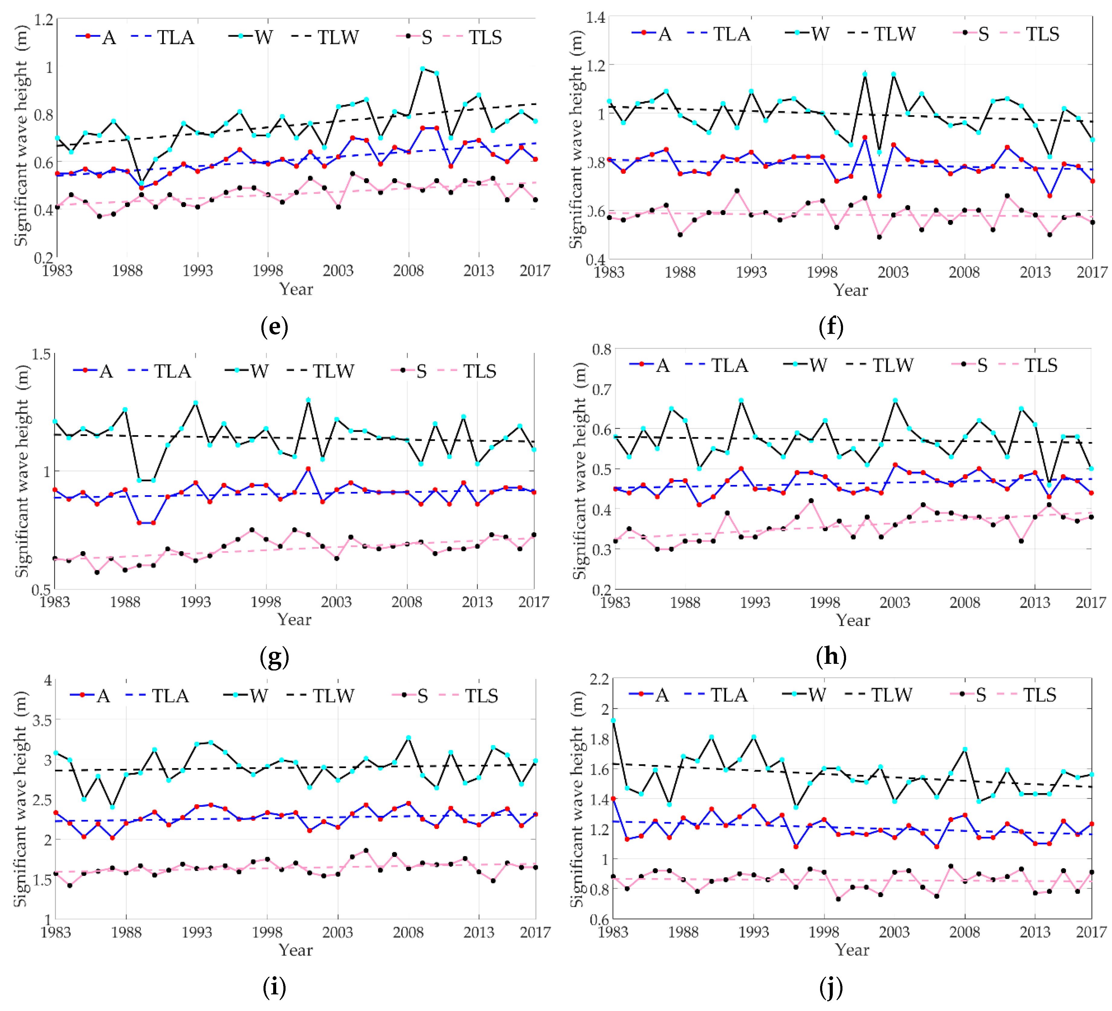
A comparison between the annual, winter, and summer season averages for the parameters U10 and Hs was carried out.

The results coming from the wind analysis show that in most of the cases, the differences between the winter and summer seasons as regards the wind speed average values are in the range 1.43–1.85 m/s. On the other hand, much higher differences for the average wind speed are noticed in the northern part of the Europe, where these can have values up to 2 m/s. The results of the wave analysis show that the differences between the winter and summer averages are in the range 0.29–0.7 m in about 90% of the cases (Reference Points H2, E3, D3, B1, F1, G1, C4, A3, and J2). Nevertheless, a higher value for this difference results in the reference point I1 (1.25 m). A classification of the maximum wind and wave conditions was also performed. According to the data analyzed, in the Mediterranean and the Black seas, quite a few events were noticed that can be classified as extreme in comparison with the North Sea. Here, 228 potential dangerous events were noticed, during which the parameter U10 had values in the range 18.8–35.2 m/s. Although the wind speed reached high intensity, the parameter Hs never crossed the upper limit of the C9 class (10 m).

Topics concerning climate change, although they are not necessarily new, have had an important dimension in the few last years. The effects can be noticed at both global and local scales. As an example, the wind analyses of Brayshaw et al. [43] and Pryor and Barthelmie [44] in the north of Europe suggest the fact that climate change can influence in a visible way the wind dynamics. An analysis of the climate change impact on the wind conditions was performed also by Schlott et al. [45]. On the other hand, the study performed by Reeve et al. 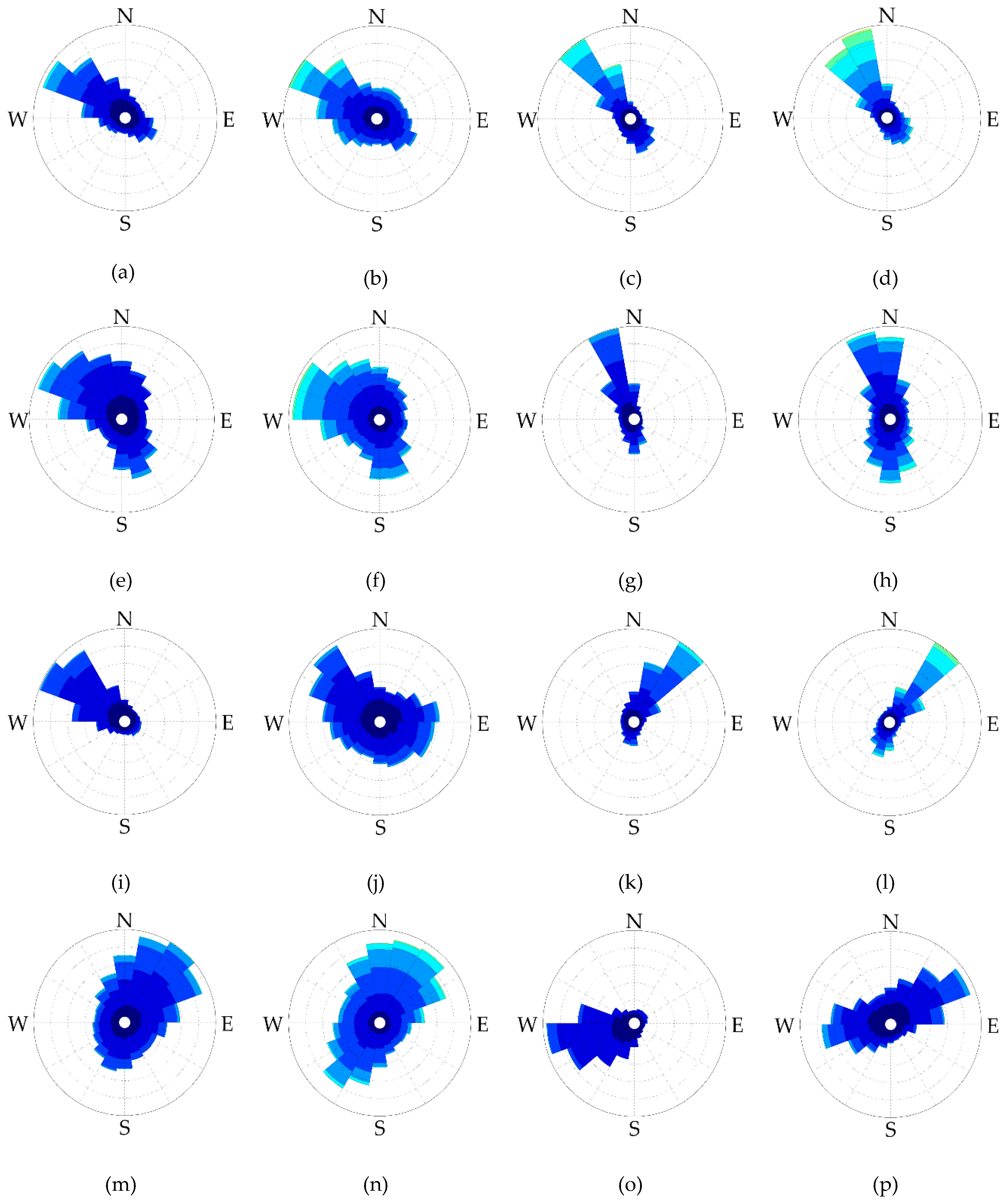[46] was focused on the effect of climate change over the wave conditions. Their results indicated a tendency of enhancement of the wave energy, a fact noticed also in the present work. At this point, we can also notice that the symmetry in the wind data was studied by many authors considering various databases, as for example [2,47,48]. Furthermore, besides providing a quantitative distribution, the present work also highlights the linear trends for the wave and wind conditions, as well as the extreme values of the wind speed and significant wave height.

At this point, the fact has to be also highlighted that there are several practical applications coming from the present work. Thus, a better perspective of the wind and wave climate and of their expected dynamics along the European sea coasts is particularly important for providing a more effective support to the coastal navigation and harbor operations. In this way, marine and coastal hazards can be better prevented [49,50,51]. Furthermore, another important direction of practical application of the results provided by the present work is related to the support for the studies focused on the marine renewable energy. This issue represents one of the greatest challenges of this century since marine renewable energy is abundant, and it is considered to be one of the most viable directions for reducing the green house effects. At this moment, the offshore wind has already become effective from an economical point of view [1,2,3,52], and this is expected to give momentum and accelerate also the development of the technologies for extracting wave energy. Moreover, the marine energy parks can represent an effective solution also for coastal protection [53,54].

Finally, it can be concluded that the present work, providing a global perspective of the main wind and wave parameters along the European sea coasts, can become also a useful reference for estimating the climate change dynamics in the areas targeted. This issue is particularly important in the marine and coastal environments, where the effects of the climate change are obviously having a stronger impact.

References

1. Wind in power 2017. Annual Combined Onshore and Offshore wind Energy Statistics. Available online: https://windeurope.org/wp-content/uploads/files/about-wind/statistics/WindEurope-Annual-Statistics-2017.pdf (accessed on 30 June 2018).
2. Onea, F.; Rusu, L. Evaluation of some State-Of-The-Art Wind technologies in the Nearshore of the Black Sea. Energies 2018, 11, 2452. [Google Scholar] [CrossRef]
3. Ganea, D.; Mereuta, E.; Rusu, L. Analysis of the present and near future wind conditions in the western side of the Black Sea. J. 2018, 18, 127–133. [Google Scholar] [CrossRef]
4. Elnaggar, M.; Edwan, E.; Ritter, M. Wind energy potential of Gaza using small wind turbines: A feasibility study. Energies 2017, 10, 1229. [Google Scholar] [CrossRef]
5. Makris, C.; Galiatsatou, P.; Tolika, K.; Anagnostopoulou, C.; Kombiadou, K.; Prinos, P.; Velikou, K.; Kapelonis, Z.; Tragou, E.; Androulidakis, Y.; et al. Climate change effects on the marine characteristics of the Aegean and Ionian Seas. Ocean Dyn. 2016, 66, 1603–1635. [Google Scholar] [CrossRef]
6. Ganea, D.; Rusu, L.; Mereuta, E. Study of the winter extreme wind in the Black Sea in the context of the climate changes. J. 2018, 18, 659–665. [Google Scholar] [CrossRef]
7. Onea, F.; Raileanu, A.; Rusu, E. Evaluation of the wind energy potential in the coastal environment of two enclosed seas. Adv. Meteorol. 2015. [Google Scholar] [CrossRef]
8. Ganea, D.; Amortila, V.; Mereuta, E.; Rusu, E. A joint evaluation of the wind and wave energy resources close to the Greek Islands. Sustainability 2017, 9, 1025. [Google Scholar] [CrossRef]
9. Sun, Z.; Sessarego, M.; Chen, J.; Shen, W.Z. Design of the off wind China 5 MW wind turbine rotor. Energies 2017, 10, 777. [Google Scholar] [CrossRef]
10. Vinoth, J.; Young, I.R. Global estimates of extreme wind speed and wave height. J. Clim. 2011, 24, 1647–1665. [Google Scholar] [CrossRef]
11. Bray, L.; Reizopoulou, S.; Voukouvalas, E.; Soukissian, T.; Alomar, C.; Vázquez-Luis, M.; Deudero, S.; Attrill, M.J.; Hall-Spencer, J.M. Expected effects of offshore wind farms on Mediterranean marine life. J. Mar. Sci. Eng. 2016, 4, 18. [Google Scholar] [CrossRef]
12. Silva, D.; Rusu, E.; Soares, C.G. Evaluation of various technologies for wave energy conversion in the portuguese nearshore. Energies 2013, 6, 1344–1364. [Google Scholar] [CrossRef]
13. Wang, T.; Yang, Z.; Wu, W.-C.; Grear, M. A Sensitivity Analysis of the Wind Forcing Effect on the Accuracy of Large-Wave Hindcasting. J. Mar. Sci. Eng. 2018, 6, 139. [Google Scholar] [CrossRef]
14. Rusu, L.; Onea, F. Assessment of the performances of various wave energy converters along the European continental coasts. Energy 2015, 82, 889–904. [Google Scholar] [CrossRef]
15. Rusu, E. Evaluation of the wave energy conversion efficiency in various coastal environments. Energies 2014, 7, 4002–4018. [Google Scholar] [CrossRef]
16. Verbrugghe, T.; Stratigaki, V.; Troch, P.; Rabussier, R.; Kortenhaus, A. A Comparison Study of a Generic Coupling Methodology for Modeling Wake Effects of Wave Energy Converter Arrays. Energies 2017, 10, 1697. [Google Scholar] [CrossRef]
17. Rusu, E.; Onea, F. Estimation of the wave energy conversion efficiency in the Atlantic Ocean close to the European islands. Renew. Energy 2016, 85, 687–703. [Google Scholar] [CrossRef]
18. Zanopol, A.T.; Onea, F.; Rusu, E. Coastal impact assessment of a generic wave farm operating in the Romanian nearshore. Energy 2014, 72, 652–670. [Google Scholar] [CrossRef]
19. Zanopol, A.T.; Onea, F.; Rusu, E. Evaluation of the coastal influence of a generic wave farm operating in the Romanian nearshore. J. Environ. Prot. Ecol. 2014, 15, 597–605. [Google Scholar]
20. Zhao, X.; Ning, D.; Zhang, C.; Liu, Y.; Kang, H. Analytical study on an oscillating buoy wave energy converter integrated into a fixed box-type breakwater. Math. Probl. Eng. 2017, 1–9. [Google Scholar] [CrossRef]
21. Rusu, L.; Onea, F. The performance of some state-of-the-art wave energy converters in locations with the worldwide highest wave power. Renew. Sustain. Energy Rev. 2017, 75, 1348–1362. [Google Scholar] [CrossRef]
22. Rusu, E.; Onea, F. Study on the influence of the distance to shore for a wave energy farm operating in the central part of the Portuguese nearshore. Energy Convers. Manag. 2016, 114, 209–223. [Google Scholar] [CrossRef]
23. The European Environment Agency (EEA). Available online: https://ec.europa.eu/eurostat/statistics-explained/index.php?title=Main_Page (accessed on 30 May 2018).
24. Wan, Y.; Fan, C.; Zhang, J.; Meng, J.; Dai, Y.; Li, L.; Sun, W.; Zhou, P.; Wang, J.; Zhang, X. Wave energy resource assessment off the coast of China around the Zhoushan islands. Energies 2017, 10, 1320. [Google Scholar] [CrossRef]
25. Alves, J.H.G.M; Young, I.R. On estimating extreme wave heights using combined Geosat, Topex/Poseidon and ERS-1 altimeter data. Appl. Ocean Res. 2003, 25, 167–186. [Google Scholar] [CrossRef]
26. Chen, G.; Bi, S.W.; Ezraty, R. Global structure of extreme wind and wave climate derived from TOPEX altimeter data. Int. J. Remote Sens. 2004, 24, 1005–1018. [Google Scholar] [CrossRef]
27. Panchang, V.; Zhao, L.; Demirbilek, Z. Estimation of extreme wave heights using GEOSAT measurements. Ocean Eng. 1998, 26, 205–225. [Google Scholar] [CrossRef]
28. Ansell, A.D.; Gibson, R.N.; Barnes, M. An Annual Review Oceanography and Marine Biology; Taylor & Francis: Abingdon, UK, 2005; p. 439. [Google Scholar]
29. Ganea, D.; Mereuta, E.; Rusu, L. Estimation of the near future wind power potential in the Black Sea. Energies 2018, 11, 3198. [Google Scholar] [CrossRef]
30. Janssen, P.A.E.M.; Hansen, B.; Bidlot, J.-R. Verification of the ECMWF wave forecasting system against buoy and altimeter data. Weather Forecast. 1997, 12, 763–784. [Google Scholar] [CrossRef]
31. ECMWF ERA-Interim. Available online: https://www.ecmwf.int (accessed on 30 June 2018).
32. WAMDI Group. The WAM model—A third generation ocean wave prediction model. J. Phys. Oceanogr. 1988, 18, 1775–1810. [Google Scholar] [CrossRef]
33. Lishaev, P.N.; Knysh, V.V.; Korotaev, G.K. Reproduction of variability of the Black Sea level and pycnocline characteristics based on the adaptive statistics method. Phys. Oceangr. 2018, 25, 251–261. [Google Scholar]
34. Torralba, V.; Doblas-Reyes, F.J.; Gonzalez-Reviriego, N. Uncertainty in recent near-surface wind speed trends:A global reanalysis intercomparison. Environ. Res. Lett. 2017, 12, 114019. [Google Scholar] [CrossRef]
35. Holthuijsen, L.H. Waves in Oceanic and Coastal Waters; Cambridge University Press: Cambridge, UK, 2007. [Google Scholar]
36. Onea, F.; Deleanu, L.; Rusu, L.; Georgescu, C. Evaluation of the wind energy potential along the Mediterranean Sea coasts. Energy Explor. Exploit. 2016, 34, 766–792. [Google Scholar] [CrossRef]
37. Rusu, L. Assessment of the wave energy in the Black Sea based on a 15-Year hindcast with data assimilation. Energies 2015, 8, 10370–10388. [Google Scholar] [CrossRef]
38. Rusu, E. The synergy between wind and wave power along the coasts of the Black Sea. In Maritime Transportation Harvesting of Sea Resources; Taylor & Francis Group: London, UK, 2016; Volume 2, pp. 1211–1217. [Google Scholar]
39. Bjorkqvist, J.V.; Lukas, I.; Alari, V.; van Vledder, Gh.; Hulst, S.; Pettersson, S.; Behrens, S.; Mannik, A. Comparing a 41-year model hindcast with decades of wave measurements from the Baltic Sea. Ocean Eng. 2018, 152, 57–71. [Google Scholar] [CrossRef]
40. Douglas Scale. Available online: http://www.eurometeo.com/english/read/doc_douglas (accessed on 30 March 2018).
41. Aydoğan, B.; Ayat, B. Spatial variability of long-term trends of significant wave heights in the Black Sea. Appl. Ocean Res. 2018, 79, 20–35. [Google Scholar] [CrossRef]
42. Lavidas, G.; Venugopal, V. Application of numerical wave models at European coastlines: A review. Renew. Sustain. Energy Rev. 2018, 92, 489–500. [Google Scholar] [CrossRef]
43. Brayshaw, D.J.; Troccoli, A.; Fordham, R.; Methven, J. The impact of large scale atmospheric circulation patterns on wind power generation and its potential predictability: A case study over the UK. Renew. Energy 2011, 36, 2087–2096. [Google Scholar] [CrossRef]
44. Pryor, S.C.; Barthelmie, R.J. Climate change impacts on wind energy: A review. Renew. Sustain. Energy Rev. 2010, 14, 430–437. [Google Scholar] [CrossRef]
45. Schlott, M.; Kies, A.; Brown, T.; Schramm, S.; Greiner, M. The impact of climate change on a cost-optimal highly renewable European electricity network. Appl. Energy 2018, 230, 1645–1659. [Google Scholar] [CrossRef]
46. Reeve, D.E.; Chen, Y.; Pan, S.; Magar, V.; Simmonds, D.J.; Zacharioudaki, A. An investigation of the impacts of climate change on wave energy generation: The Wave Hub, Cornwall, UK. Renew. Energy 2011, 36, 2404–2413. [Google Scholar] [CrossRef]
47. Neill, S.P.; Hashemi, M.R. Wave power variability over the northwest European shelf seas. Appl. Energy 2013, 106, 31–46. [Google Scholar] [CrossRef]
48. Weber, J.; Gotzens, F.; Witthaut, D. Impact of strong climate change on the statistics of wind power generation in Europe. Energy Procedia 2018, 153, 22–28. [Google Scholar] [CrossRef]
49. Gasparotti, C.; Rusu, E. Methods for the risk assessment in maritime transportation in the Black Sea basin. J. Environ. Prot. Ecol. 2012, 13, 1751–1759. [Google Scholar]
50. Rusu, L.; Guedes Soares, C. Local data assimilation scheme for wave predictions close to the Portuguese ports. J. Oper. Oceanogr. 2014, 7, 45–57. [Google Scholar] [CrossRef]
51. Butunoiu, D.; Rusu, E. Wave modeling with data assimilation to support the navigation in the Black Sea close to the Romanian ports. In Proceedings of the Second International Conference on Traffic and Transport Engineering, Belgrade, Serbia, 27–28 November 2014; pp. 180–187. [Google Scholar]
52. Onea, F.; Rusu, E. Efficiency assessments for some state of the art wind turbines in the coastal environments of the Black and the Caspian seas. Energy Explor. Exploit. 2016, 34, 217–234. [Google Scholar] [CrossRef]
53. Bento, R.; Rusu, E.; Martinho, P. Assessment of the changes induced by a wave energy farm in the nearshore wave conditions. Comput. Geosci. 2014, 71, 50–61. [Google Scholar] [CrossRef]
54. Diaconu, S.; Rusu, E. The environmental impact of a wave dragon array operating in the Black Sea. Sci. World J. 2013, 2013. [Google Scholar] [CrossRef] [PubMed]
Figure 1. The geographical locations of the target areas considered in the European coastal environment; (a) Zones A, B, C, D, E, F, G, and H correspond to the southern and southeastern parts of Europe; (b) Zones I and J correspond to the north of Europe.
Jmse 07 00043 g001
Figure 2. The geographical locations of the 40 reference points considered in the study. (a) Zones A, B, C, D, E, F, H, and G correspond to the Balearic, Ligurian, Tyrrhenian, Adriatic, Ionian, Aegean, Levantine and Black seas, respectively; (b) Zone I corresponds to the North Sea and Zone J to the Baltic Sea.
Jmse 07 00043 g002
Figure 3. Assessment of the yearly mean wind speed corresponding to the 35-year time slice resulting from processing the ECMWF ERA-Interim data. Each box includes several keys: the top and the bottom of the box represent the upper and lower quartiles, so the box spans the interquartile range; the median is marked by a vertical red line placed inside of the box; the whiskers are the lines (two) outside the box that extend to the highest (upper extreme) and lowest (lower extreme) observations; the outliers are those observations that are numerically distant from the rest of the data (red crosses); the mean values are represented by black dots; (a) Reference points A–E; (b) Reference points F–J.
Jmse 07 00043 g003
Figure 4. Distribution of the U10 wind speed in the sites considered, as resulting from the analysis of the ECMWF ERA-Interim dataset for the time interval 1983–2017. The data were processed in terms of maximum values, 95th percentile, and average values in comparison to the upper four wind classes (C9–C12) of the Beaufort scale.
Jmse 07 00043 g004
Figure 5. Representation of the wind speed (U10) for the annual averages (A), winter (W) and summer (S) seasons corresponding to the most representative points; (a) A3, Balearic Sea; (also) B1, Ligurian Sea; (c) C4, Tyrrhenian Sea; (d) D3, Adriatic Sea; (e) E3, Ionian Sea; (f) F1, Aegean Sea; (g) G1, Black Sea; (h) H2, Levantine Sea; (i) I1, North Sea; and (j) J2, Baltic Sea. TLA represents the trend line for the annual averages, while TLW and TLS are the trend lines for the winter and summer seasons, respectively. Results corresponding to the35-year time interval 1983–2017.
Jmse 07 00043 g005aJmse 07 00043 g005b
Figure 6. Assessment of the yearly mean significant wave height corresponding to the 35-year time slice (corresponding to the time interval 1983–2017) resulting from processing the ECMWF ERA-Interim data. Each box includes several keys: the top and the bottom of the box represent the upper and lower quartiles, so the box spans the interquartile range; the median is marked by a vertical red line placed inside of the box; the whiskers are the lines (two) outside the box that extend to the highest (upper extreme) and lowest (lower extreme) observations; the outliers are those observations that are numerically distant from the rest. (a) Reference points A–E; (b) Reference points F–J.
Jmse 07 00043 g006
Figure 7. Distribution of the Hs wave conditions in the sites considered, for the ECMWF ERA-Interim dataset, corresponding to the time interval 1983–2017. The data were processed in terms of maximum values, 95th percentile, and average values in comparison to the upper three wind classes (C6–C8) of the Douglas Scale.
Jmse 07 00043 g007
Figure 8. Representation of the significant wave height (Hs) for the annual averages (A), winter (W), and summer (S) seasons corresponding to the most representative points; (a) A3, Balearic Sea; (b) B1, Ligurian Sea; (c) C4, Tyrrhenian Sea; (d) D3, Adriatic Sea; (e) E3, Ionian Sea; (f) F1, Aegean Sea; (g) G1 Black Sea; (h) H2, Levantine Sea; (i) I1, North Sea; and (j) J2, Baltic Sea. TLA represents the trend line for the annual averages, while TLW and TLS are the trend lines for the winter and summer seasons, respectively. Results corresponding to the 35-year time interval 1983–2017.
Jmse 07 00043 g008aJmse 07 00043 g008b
Figure 9. Representation of significant wave height (Hs) and wind speed histograms (U10) in comparison with the normal distribution for ten of the most representative points: (a) A3; (b) B1; (c) C4; (d) D3; I E3; (f) F1; (g) G1; (h) H2; (i) I1, and (j) J2.
Jmse 07 00043 g009
Figure 10. Wind roses corresponding to the two seasons (winter and summer), resulting from processing the data for the 35-year period considered. The results are provided for ten of the most representative locations, one for each geographical zone targeted. (a) summer season-A3; (b) winter season-A3; (c) summer season-B1; (d) winter season-B1; (e) summer season-C4; (f) winter season-C4; (g) summer season-D3; (h) winter season-D3; (i) summer season-E3; (j) winter season-E3; (k) summer season-F1; (l) winter season-F1; (m) summer season-G1; (n) winter season-G1; (o) summer season-H2; (p) winter season-H2; (q) summer season-I1; (r) winter season-I1; (s) summer season-J2; (t) winter season-J2.
Jmse 07 00043 g010aJmse 07 00043 g010b