Nearshore Wave Dynamics at Mangalia Beach Simulated by Spectral Models

Abstract

The objective of this paper is to present an integrated picture of the relationship between the waves and the modifications induced by them in the Romanian shoreline. Thus, the hydrodynamic processes at the Mangalia beaches, located in the southern side of the Romanian nearshore, are simulated using the modeling system Mike 21 SW (MIKE 21 Spectral Waves), developed by the Danish Hydration Institute (DHI). This is one of the newest spectral wave models, which can be used for regional- and local-scale simulations. The model has been calibrated and validated using buoy measurements. The analysis of the statistical parameters shows a good match between the model and the observed data. Furthermore, a model to compare the differences that occur on the beach profiles between the cold and warm seasons was developed. The results obtained indicate a reinforcement of the coastal erosion in the winter, when the waves are stronger (especially in January and February).

1. Introduction

Hydrodynamic processes occurring in the marine environment are a consequence of the complex interactions between the sea and the atmosphere, and waves are generated by the interaction between the wind and the sea surface [1]. For this reason, the system evolution and phenomena occurring along coastlines are difficult to simulate with numerical models, and a proper implementation of wave models is very important [2]. Prediction of sea state conditions in the proximity of coastlines is quite difficult due to the various processes of wave transformation, which are influenced by, among others, the bathymetry of the area, the locations of the hydrotechnical structures, and the regime of wind and currents [3].

Numerical models are essential tools to simulate the wave conditions in coastal areas, providing information on the wave climate that helps the design of the coastal structures, which can protect the coastal areas during extreme events. Coastal environments have often been the subject of several spectral wave models for various studies related to wave hindcast or forecast. The model MIKE 21 SW (MIKE 21 Spectral Waves) is one of the newest spectral wave models used to simulate the physical processes related to the generation and transformation of wind waves [4]. A calibration and validation of the wave model results is necessary to ensure that reliable information is obtained, and at this step, some obstacles occur due to difficulties in obtaining the field data. The measurements are also important to obtain information regarding the wave climate in a location/area and the evolution of the coastal erosion phenomenon that intensifies and threatens the inhabited areas.

The MIKE 21 SW model has been implemented in different marine environments of the world, showing to be an efficient tool. For example, the Indian National Ocean Service Information Center implemented the MIKE 21 SW model in the Indian Ocean, and it has been used for wave predictions during a cyclone. The comparisons performed against buoy measurements indicated a good agreement between them [5]. The effects of storm waves on some beaches located in Brazil and the Gulf of Mexico have been studied, also using the results of the MIKE 21 SW model [6,7]. In another study, the results provided in the Persian Gulf by two wave models, namely MIKE 21 SW and WAVEWATCH III, were compared. The comparisons showed that in deep water, better results are obtained with WAVEWATCH-III, while in shallow water, better results are obtained with MIKE 21 SW [8]. The sea state conditions in the Black Sea basin have been also simulated with the MIKE 21 SW model in order to study the spatiotemporal variability of the wave climate over an extended time period covering 37 years [9].

Harvesting ocean energy represents a promising topic, and the ocean energy potential can be assessed based on the results provided by the numerical models that can also provide guidance regarding the places with the best wave energy resources [10,11]. For this purpose, MIKE 21 SW was used to calculate the wave energy potential in the Black Sea [12] and the Aegean Sea [13]. The model results in the Black Sea at various locations show that better results can be obtained with MIKE 21 SW for the wavelengths than for the wave periods.

The Romanian coastline has a length of about 243 km in the western part of the Black Sea. The limits are given by the border with Ukraine (in the bay of Musura) to the North, and the border with Bulgaria (near Vama Veche) to the South. At present, the Romanian seaside does not benefit from many field measurements of the wave parameters.

The coastal geomorphology of the Romanian shore can be divided in two large units/areas with different sediment balance that differently react to the actions of the main environmental factors [14]. Thus, the first unit (the Northern unit) stretches from Musura Bay to Midia Harbor (including the Danube Delta, with the lake complex Razim–Sinoe), and covers a length of about 160 km and is characterized by low beaches in the delta/lagoon and slope submarine lines. Over time, the Danube Delta has suffered from numerous accretion processes (the Sulina Lob, which is about 12 km wide) and erosion (Delta St. George II and Chilia) [15].

The Southern unit has a different shape, with soft rock cliffs (loess) and pocket beaches. These beaches have steeper slopes than those in the Northern unit. The Southern unit is also characterized by various deposits of sediments (where the rocks in the basement appear on the surface of the earth’s crust due to erosion), predominantly those of the Sarmatian limestone age. Over these limestones, there are layers of Pleistocene clay covered with deposits of loess and paleosols [16]. These types of sediment lead to the formation of unstable cliffs with deposits of siltic sediments and very fine sands. The beaches in front of the cliffs are rockier, with reduced quantities of medium-sized granular sediments. This is due to the construction of the Midia harbor that has modified the sediment transport patterns, which has led to the implementation of some beach nourishment projects [17].

The target area of the present work is a coastal sector near the Mangalia port, located in the Southern part of the Romanian seashore. The implementation and calibration of the MIKE 21 SW model in the target area represents the main objective of the work. An analysis of the wave climate, wave seasonality, and how the sea state conditions affect the Mangalia beach is also carried out, based on the simulation results.

2. Materials and Methods

2.1. Target Area

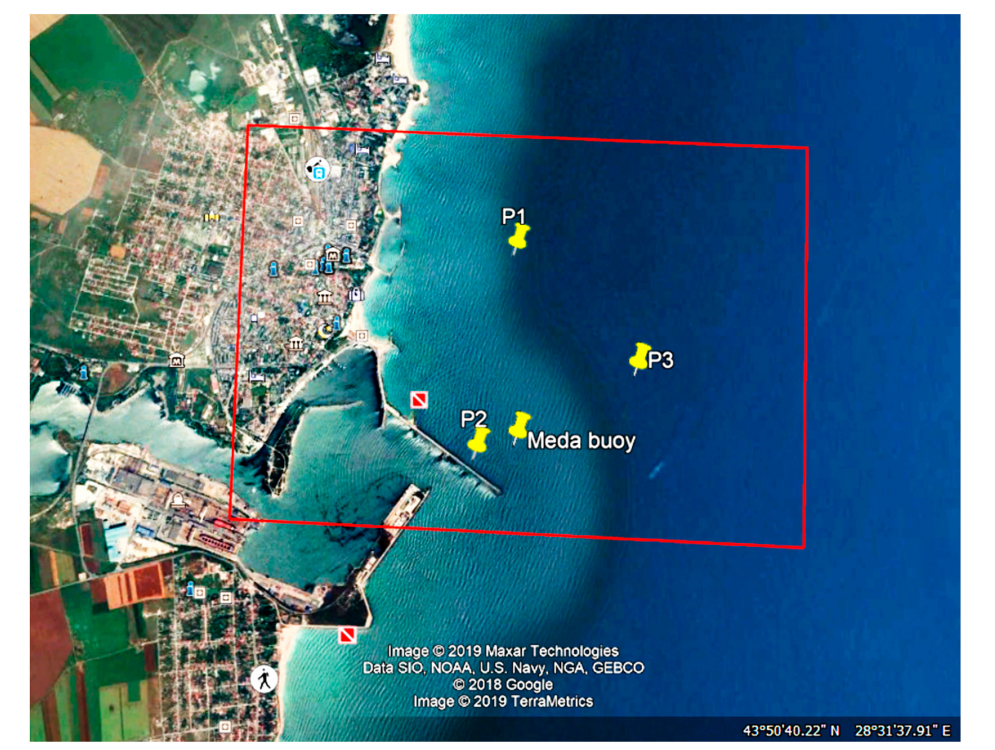
Mangalia port, the target area of this study (Figure 1), is extremely important for the national, regional, and local economy, and is also important from a social perspective, being the major source of jobs in the coastal area. This harbor is located on the Southern part of the Romanian coastline, being protected by dikes built during the period of 1970–1980 that have altered the coastal dynamics of the Southern unit over time. The coastal alluvial transport direction is towards the south, but the existence of levees and other coastal development projects induces different local patterns. The construction of the port of Mangalia also affected the southern beaches and cliffs from 2 Mai to Vama Veche (two small villages located on the Romanian coastline) [12]. For this case study, where the erosion rate is visible (as proved by the research carried out for the elaboration of the Coastal Master Plan [14]), the MIKE 21 SW was implemented in order to analyze the phenomena occurring in the nearshore.

2.2. Wave Model

The MIKE 21 SW modeling system [4], developed by the Danish Hydration Institute (DHI), Hørsholm, Denmark, is a numerical tool with capabilities to simulate and analyze the wave climate in offshore and coastal areas. The wave model uses the unstructured mesh technique to define the geographical domain.

The governing equation of this model is based on a wave action density spectrum $N\left(\sigma , \theta \right)$, where $\sigma$ is the independent phase parameter (the relative angular frequency) and $\theta$ is the direction of wave propagation. The action density, $N\left(\sigma , \theta \right)$, is dependent on energy density [4].

$$N\left(\sigma , \theta \right)=\frac{E}{\sigma }.$$

(1)

MIKE 21 SW includes two types of formulations: Directional decoupling and full spectral. The first formulation is based on the parameterization of the wave action conservation equation and is more appropriate for nearshore processes, while the second formulation is also suitable for the offshore area. Parameterization is performed in a frequency range by inputting the zero moment and the first momentum of the wave action spectrum as parameters. The wave action balance equation is formulated in Cartesian or spherical coordinates.

$$\frac{\partial N}{\partial t}+\nabla ·\left(\overline{\nu }N\right)=\frac{S}{\sigma },$$

(2)

where $N\left(\overline{x},\sigma ,\theta ,t\right)$ is the action density, t is the time, $\overline{x}=\left(x,y\right)$ are the Cartesian coordinates, and $\overline{\nu }=\left(c_x,c_y, c_{\sigma }, c_{\theta }\right)$ is the propagation velocity of a wave group in the four-dimensional phase space $\overline{x}, \sigma ,$ and $\theta .$S is the source term for the energy balance equation, and $\nabla$ is the four-dimensional differential operator in the $\overline{x}, \sigma ,$ and $\theta$ space.

The full spectral formulation is also based on the wave action conservation equation, where the waveform spectrum of directional frequency is a dependent variable [18,19]. For the present study, the full spectral formulation was chosen.

The MIKE 21 SW module simulates variable flow, taking into account the bathymetry, sources, and external forces. Bathymetric data were obtained, retrieved, and processed in an XYZ format from old bathymetric maps, and then they were added in the Mesh Generator module. The bathymetric data resolution was 0.001°. While the field and boundaries were defined in the MIKE Zero Mesh Generator and the interpolation was running, the boundary conditions were excluded. In addition, the points were interpolated by the adjacent value and the values for those points were set.

2.2.1. Unstructured Mesh Approach

The unstructured mesh approach is becoming increasingly important for coastal applications. Coastal areas require a better prediction of wave characteristics for the safe design of hydrodynamic structures. This approach makes the representation of the offshore, coastal, and harbor structures more accurate in the computational domain.

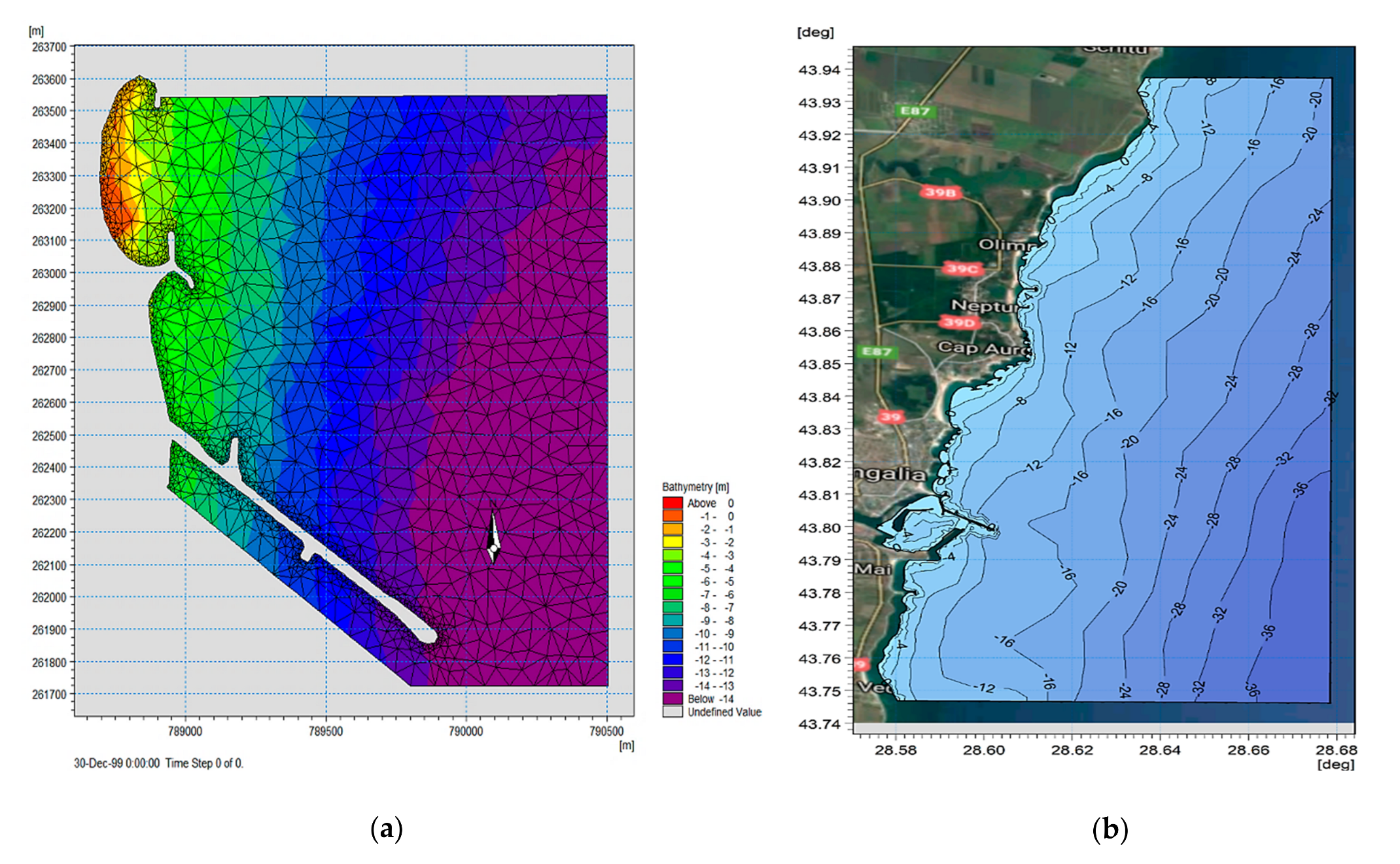
Bathymetric data were obtained, retrieved, and processed in an XYZ format from old bathymetric maps, and then added in the Mesh Generator module. The bathymetric data resolution was 0.001°. While the field and boundaries were defined in the MIKE Zero Mesh Generator and the interpolation was running, the boundary conditions were excluded. In addition, the points were interpolated by the adjacent value and the values for those points were set.

Figure 2a shows the details of this unstructured mesh, which contains the values of the nodes and mesh attributes corresponding to the bathymetric data and boundary points in the Mangalia region. Figure 2b shows the general view of detailed bathymetry in the MIKE ZERO View.

2.2.2. Initial Conditions

The spectra from empirical formulations were used as initial conditions. The parameters that influence the wave regime in the coastal zone were also considered. Among the parameters available for breaking waves, the breaking parameter $\gamma =0.8$ was specified. The mean size of the sediments in the Mangalia area was considered to be D₅₀ = 0.48 mm.

The JOint North Sea WAve Project (JONSWAP) spectrum with the fetch value of 100 km was considered, while the parameters describing the whitecapping (C_dis) and dissipation coefficient (δ) were C_dis = 3.5 and δ = 0.8, respectively.

2.2.3. Boundary Conditions

The boundary conditions for the MIKE 21 SW model are provided by the SWAN (acronym from Simulating Waves Nearshore [20]) model, a state-of-the-art wave model based on the spectrum concept. The wave modelling system based on the SWAN model has two computational levels. This wave modelling system was extensively validated by comparisons with various measurements [21,22]. The first computational level covers the entire Black Sea basin, and has a resolution of 0.08 degrees in both longitude and latitude (176 points in the x-direction and 76 points in the y-direction). The second level is focused on the Romanian nearshore, and the spatial resolution is 0.02 degrees (101 points) in both directions (see more information in [22,23]). The computational grids are structured grids and coincide with the bathymetric grids. The SWAN model was forced with the reanalysis wind fields provided by the NCEP-CFSRv2 (U.S. National Centres for Environmental Prediction—Climate Forecast System Reanalysis Version2) data base. These wind fields were used for both levels of the wave modelling system. The simulations with the SWAN model were carried out for the entire year of 2016. At the second level, the values of the wave parameters were provided in order to be used as boundary conditions for the local scale where MIKE 21 SW was implemented and calibrated.

The calibration process was performed using a waveform spectral formula (significant wave height H_s, mean wave period T_m, and mean wave direction) for the three open boundaries. The boundary conditions were obtained from SWAN simulations in three points used as limits:

• P1: x = 28.602 [deg]; y = 43.816 [deg]; depth = −11 m, North boundary;
• P2: x = 28.598 [deg]; y = 43.801 [deg]; depth = −11.95 m, South boundary; and
• P3: x = 28.614 [deg]; y = 43.807 [deg]; depth = −15.53 m, East boundary.

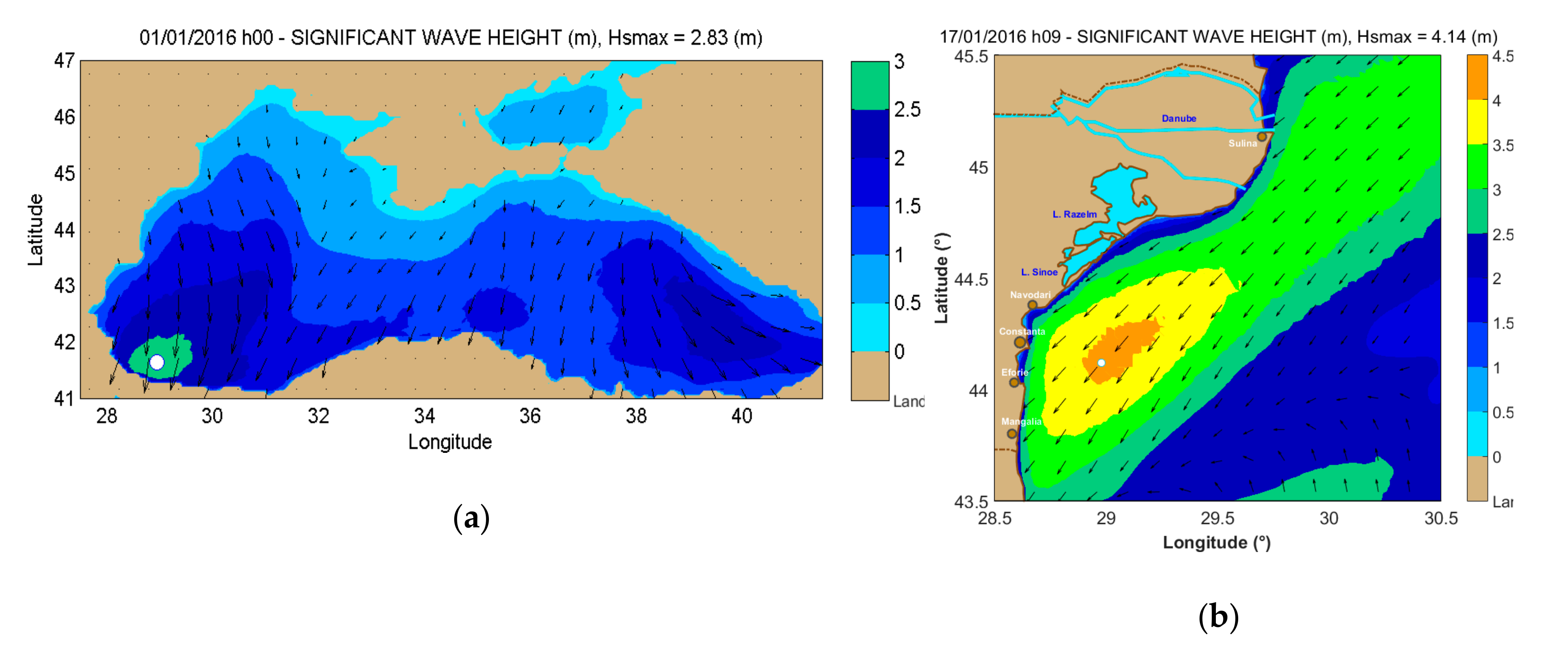
Figure 3 shows the significant wave heights in fields simulated throughout the Black Sea basin and Romanian coastal environment at different time frames.

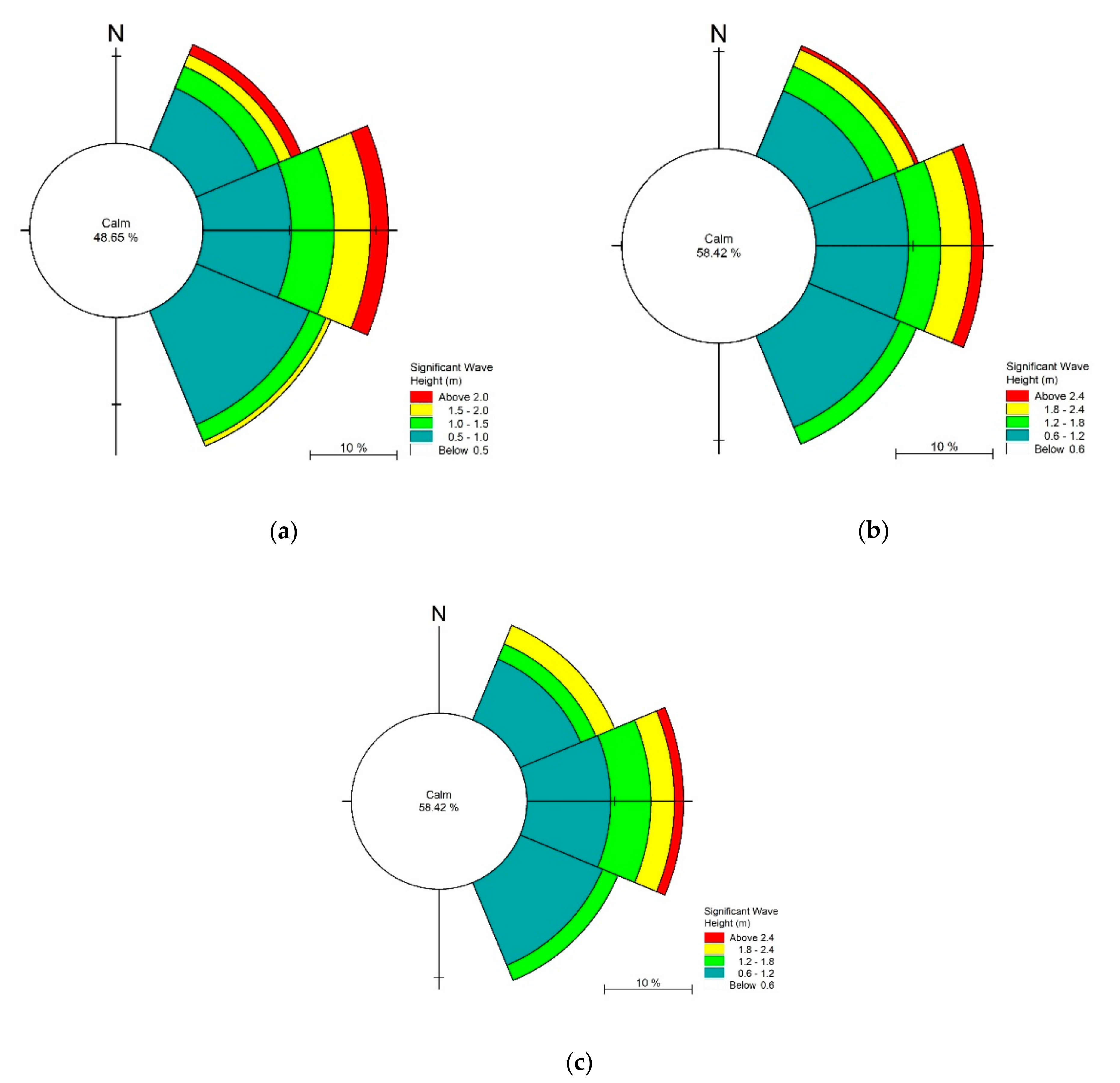
In Figure 4, the wave roses in the three locations established as limits are presented. It can be noticed that the Northern boundary (P1) has significantly lower wave heights than the Southern (P2) and the Eastern (P3) boundaries. This can be explained by the existence of protection systems in the area, which have the role of dissipating the wave energy.

2.2.4. Output Parameters

The output parameters considered are those obtained from the integration of the wave spectrum, and can be provided over the computational grid or for specific locations previously defined. The relationships of the parameters are:

1)

Significant wave height,

$$H_{m0}=4\sqrt{m_0}$$

(3)

2)

Mean wave period,

$$T_{02}=\sqrt{\frac{m_0}{m_2}}$$

(4)

• Mean wave direction, $\overline{\theta }\left(grade\right),$ considering nautical convention

$$\overline{\theta }=270-{\tan }^{-1}\frac{b}{a}$$

(5)

where,

$$\begin{array}{c}a=\frac{1}{m_0}{{\displaystyle \int }}_0^{2\pi }\underset{0}{\overset{\infty }{{\displaystyle \int }}}cos\left(\frac{3}{2}\pi -\theta \right)E\left(f,\theta \right)dfd\theta \\ b=\frac{1}{m_0}{{\displaystyle \int }}_0^{2\pi }\underset{0}{\overset{\infty }{{\displaystyle \int }}}sin\left(\frac{3}{2}\pi -\theta \right)E\left(f,\theta \right)dfd\theta \end{array}$$

(6)

The differences between wind–waves/seas and swells can be calculated using either a frequency threshold constant or a dynamic frequency with a higher frequency limit. For the present study, a constant frequency equal to 0.1 Hz was used, as in the case of data recorded from the buoy [4].

3. Results

3.1. Calibration of the Wave Model

Field data are essential to evaluate the accuracy of the model results. In this work, the Coastal Gauge (MEDA) Mangalia (Romania) buoy maintained by GeoEcoMar (National Research and Development Institute for Marine Geology and Geo-ecology) was used for the model calibration and validation. The buoy is located at latitude 43.802176° N and longitude 29.602483° E [WGS84], at a depth of 15 m (see Figure 1). The measurements were made in the framework of the project "Marine Pollution Oriented Marine Policies—PERSEUS" from OCEAN 2011-3, "Assessing and predicting the combined effects of natural and human-made pressures in the Mediterranean and the Black Sea in view of their better governance”. The project has been finished, but the wave measurement instruments installed continue to operate, and the recorded data series can be viewed using a specific FlowQuest 1000 + Wave program (LinkQuest Inc., San Diego, CA, USA), both online and offline [24].

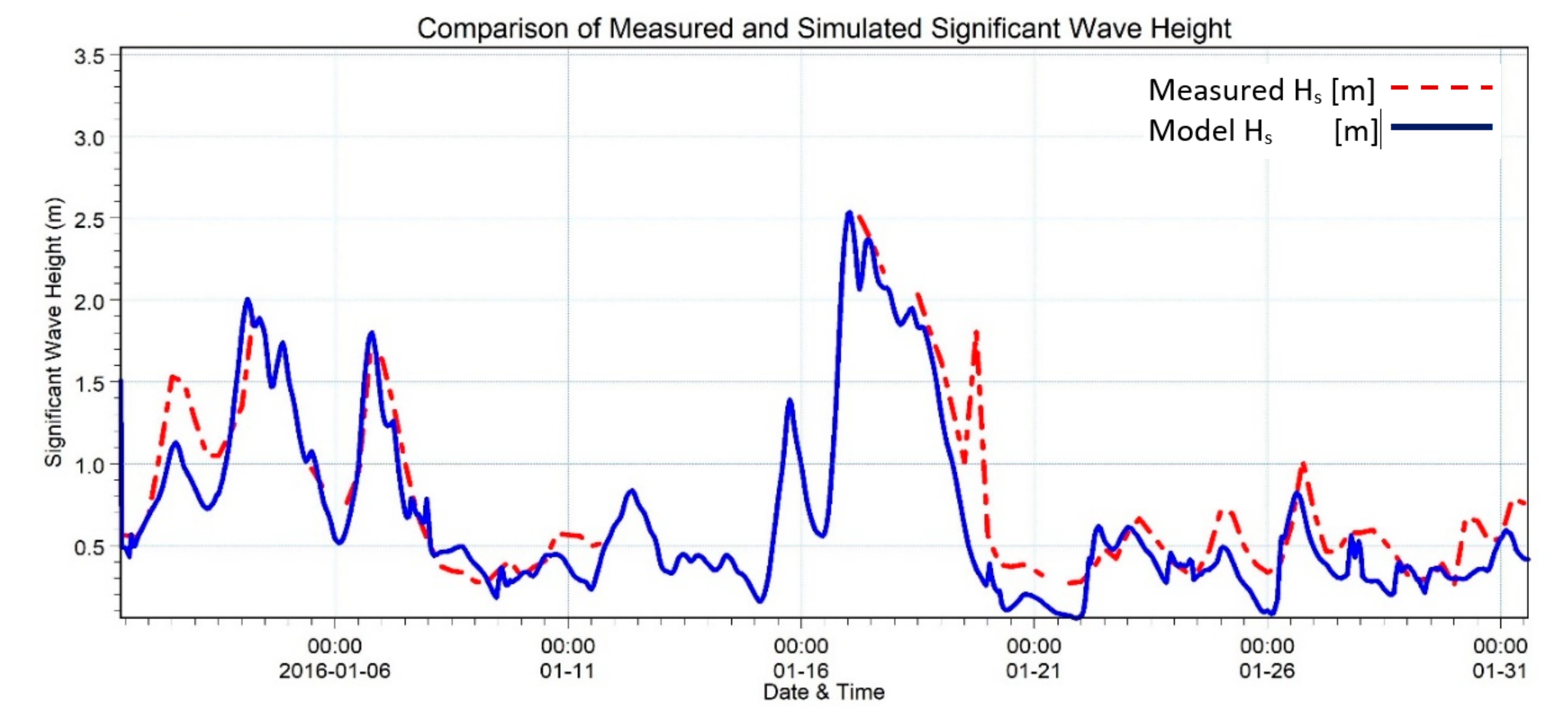
The wave model was calibrated by comparing two wave parameters, H_s—significant wave height and T_m—mean wave period, recorded by the buoy in January 2016 with those simulated by the MIKE 21 SW model at the location of the buoy. The calibration consisted of iterative adjustments of the model until the analysis module indicated a good fit between the simulated and measured wave parameters.

The comparison between the values of H_s simulated by MIKE 21 SW and H_s recorded by the buoy is presented in Figure 5, with the blue line showing the simulated values, while the red line represents the observed data. The simulated data closely match the measured data, indicating that the model simulated the wave heights well.

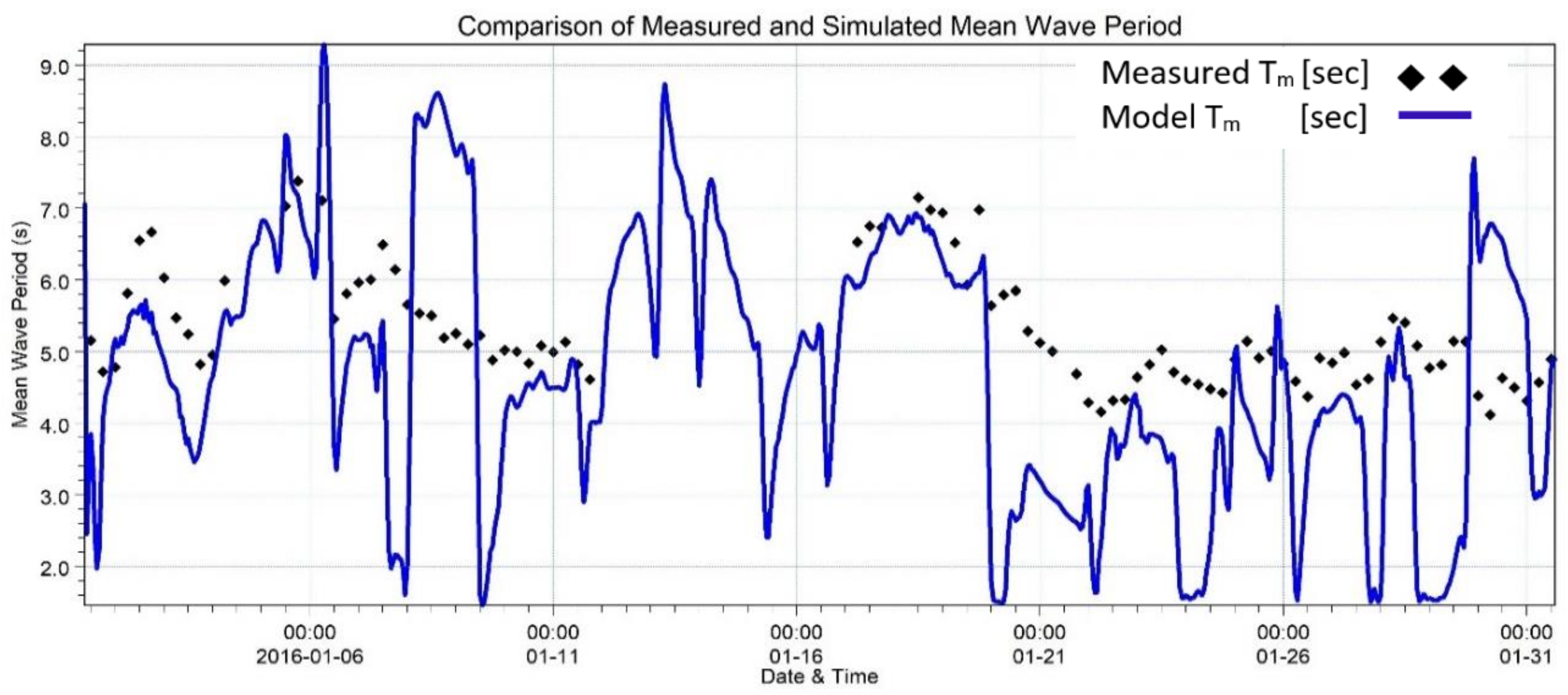
The second wave parameter investigated in this study is the mean wave period, and, as can be seen from Figure 6, the fluctuations of the simulated mean wave periods are not very different from the observed data.

One important point to be considered is the assessment of the quality of the model results, and this can be made by computing various statistical parameters.

One method is to determine the square root of the average of the squared errors between the estimated and observed values, which is known as the Root Mean Square Error (RMSE):

$$RMSE=\sqrt{\frac{{{\displaystyle \sum }}_{i=1}^N{\left(S_i-M_i\right)}^2}{N}},$$

(7)

where S represents the simulated values using the MIKE 21 SW model, M represents the values measured by the buoy, and N is the number of observations valid for this station.

A well-known statistical parameter used to evaluate how strong a relationship is between two variables is the Pearson product–moment correlation coefficient (or Pearson correlation coefficient, for short). The coefficient is computed as follows:

$$R=\frac{{{\displaystyle \sum }}_{i=1}^N\left(S_i-\overline{S}\right)\left(M_i-\overline{M}\right)}{\sqrt{{{\displaystyle \sum }}_{i=1}^N{\left(S_i-\overline{S}\right)}^2{{\displaystyle \sum }}_{i=1}^N{\left(M_i-\overline{M}\right)}^2}}.$$

(8)

Another statistical parameter widely used to compare the simulated wave parameters with those measured is BIAS, which represents the mean error:

$$BIAS={\displaystyle \sum }_{i=1}^N\frac{1}{N}\left(S_i-M_i\right).$$

(9)

Finally, the scatter index is another statistical parameter used for comparing two data sets that occurred within the same timeframe, which is computed as [25]:

$$SI=\frac{\sqrt{\frac{1}{N}{{\displaystyle \sum }}_{i=1}^N{\left(S_i-M_i\right)}^2}}{\sqrt{\frac{1}{N}{{\displaystyle \sum }}_{i=1}^N{M}_i}}·100$$

(10)

The statistical parameters presented above were considered to evaluate the accuracy of two wave parameters: The significant height (H_s) and the mean period (T_m). Their values are presented in

Table 1. Statistical parameters computed for significant wave height (H_s) and mean wave period (T_m).

Wave Parameters	R	RMSE	BIAS	SI (%)
Hs	0.953	0.200	0.040	23.19
Tm	0.769	0.678	0.460	29.64

.

As a result of these analyses, the value of the correlation index R is 0.953 for H_s and 0.769 for T_m. These values indicate a strong correlation between the simulated and measured H_s, which means that the simulated data tend to match very well with the measured data, while in the case of T_m the simulated results are less accurate.

The BIAS, RMSE, and SI statistical coefficients are considered to be better if their values are smaller (near to zero). In the case of the correlation coefficient, R, the results are when it is closer to the unit [26]. Pianc [26] sets a range for the BIAS index of between 0–0.1 for H_s and ≈ 0 for T_m, so that the data obtained correspond to the measured data. In the case of H_s, the value obtained for BIAS falls within the limits of acceptability described above. Therefore, after the analysis of all statistical parameters, it can be said that H_s in the Mangalia area was very well simulated by the MIKE 21 SW model, while in the case of T_m, more adjustments probably need to be made in order to improve the predicted values. The wave model described has a very close prediction with the wave pattern studied.

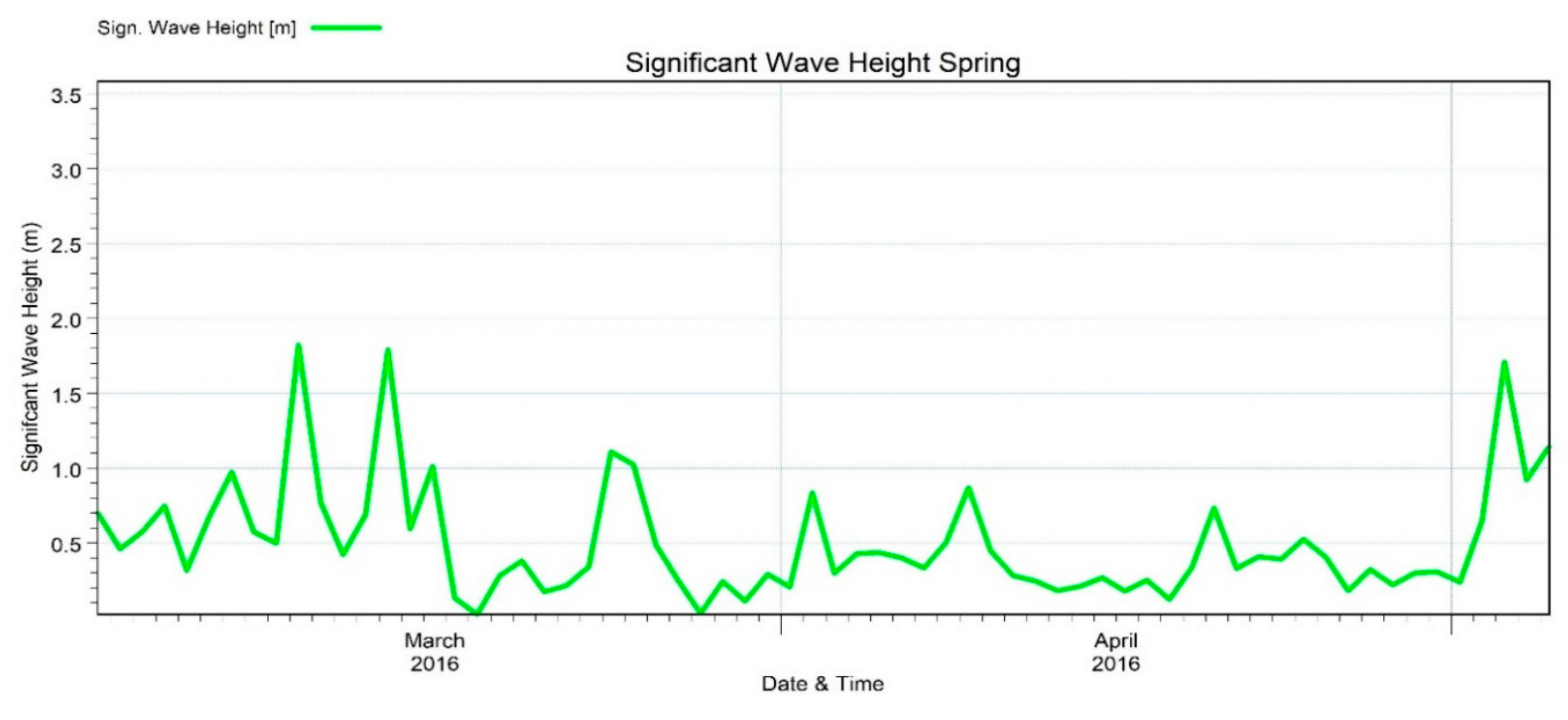
3.2. Seasonal Wave Analysis

In the following section, the seasonal variability of H_s in the Mangalia area, near to the beach area where the erosion is more pronounced during the cold season than in the warm season, is analyzed. The simulations at the local scale were performed between January and September 2016, except May, for which no wind data was recorded by the buoy located in the area. All simulations were made considering the previously calibrated model with the 12-hour interval. The Figure 7, Figure 8, Figure 9 and Figure 10 show the significant wave heights simulated for spring, summer, autumn and winter, respectively.

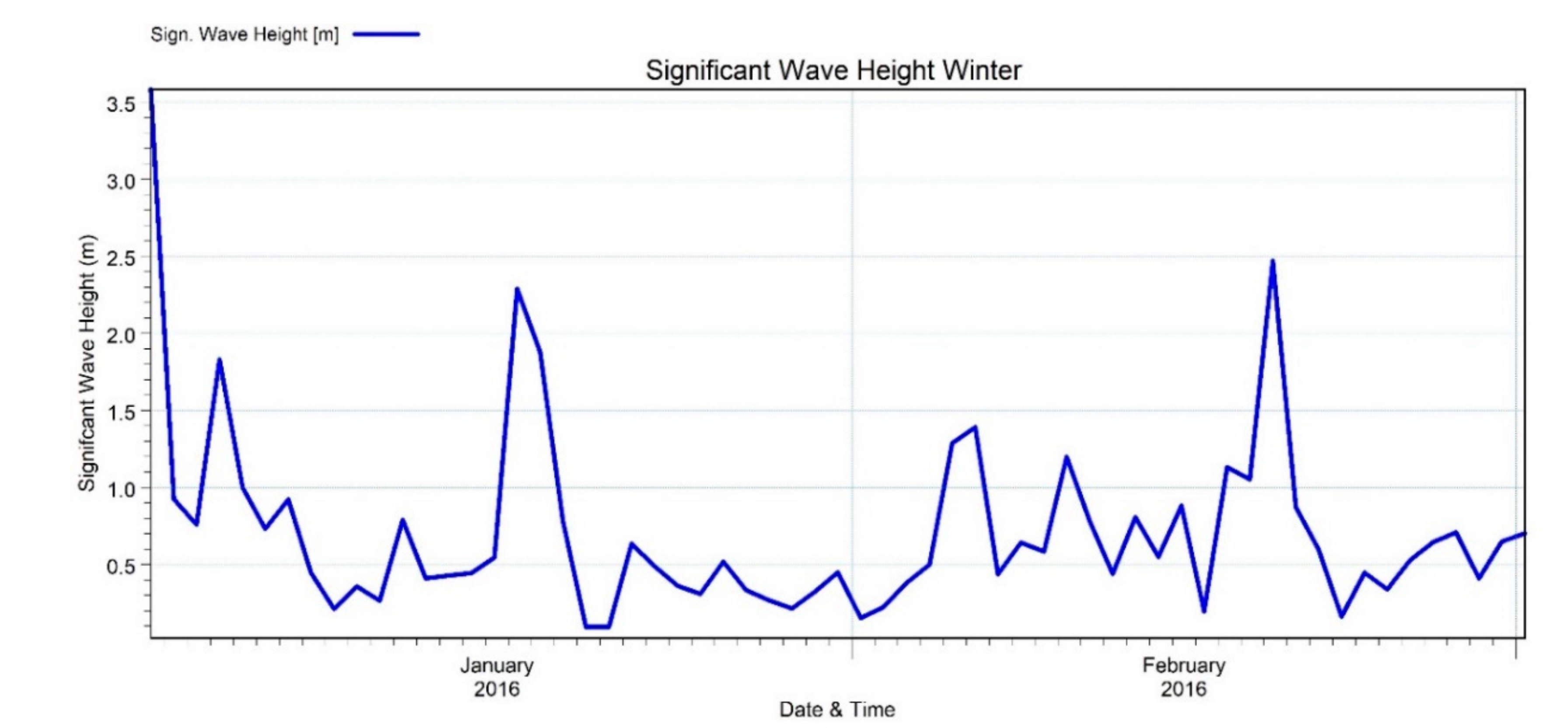
From Figure 8 and Figure 9, it can be observed that H_s values in summer and autumn are lower than 1 m, while in spring (especially in March), we can find H_s values several times higher than 1.5 m. As expected, the highest H_s values are found in winter.

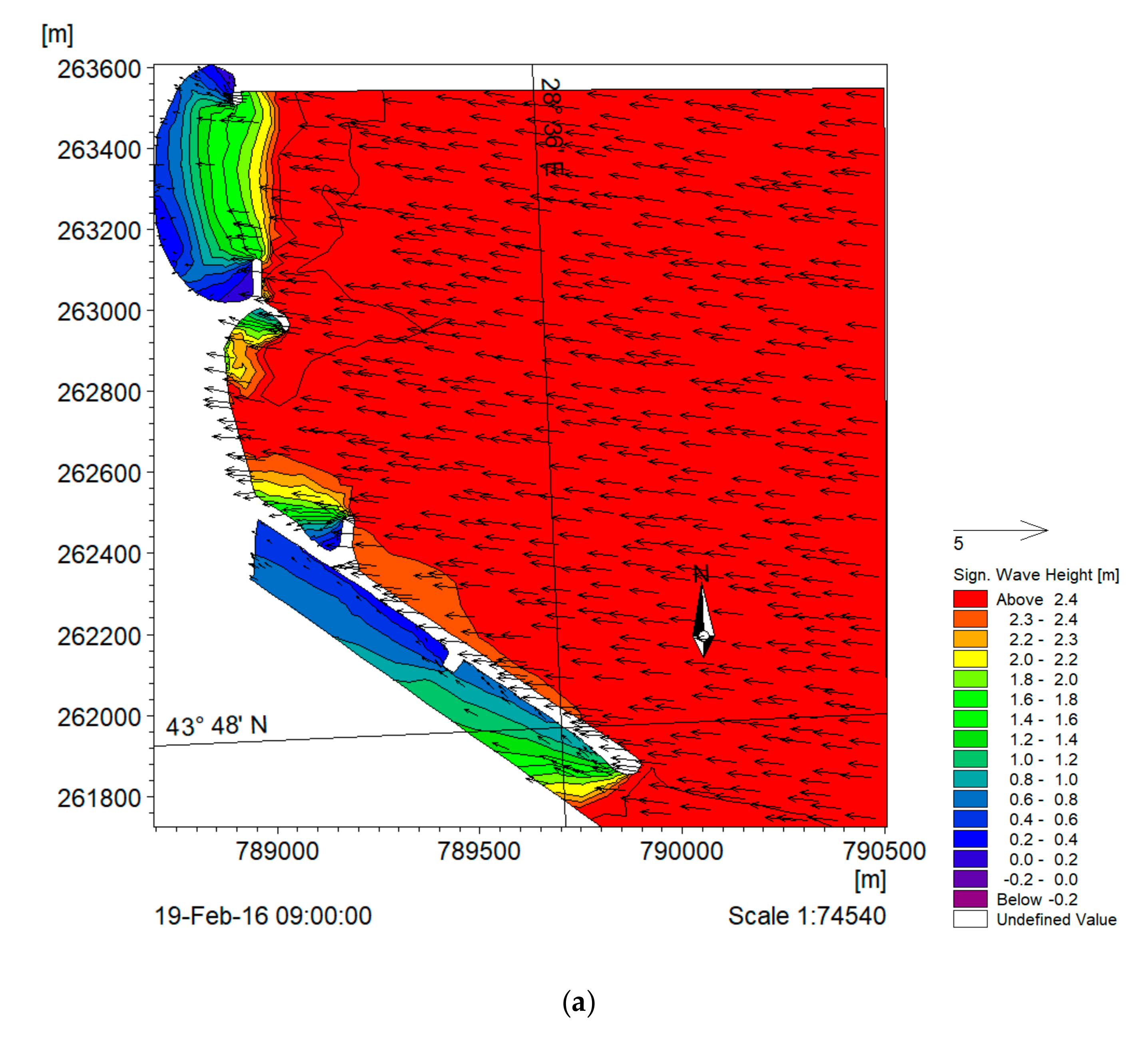
During the year 2016, the higher values of the mean H_s were in the winter months, and thus in February, the average was 0.45 m, with a maximum of 2.47 m (Figure 11a), while in January, they had an average of 0.67 m, with a maximum of 2.53 m. In the summer of 2016, the significant wave heights in the middle of the bay reached an average value of 0.36 m and a maximum of 0.89 m (Figure 11b), while T_m had an average period of 3.78 seconds.

4. Discussion

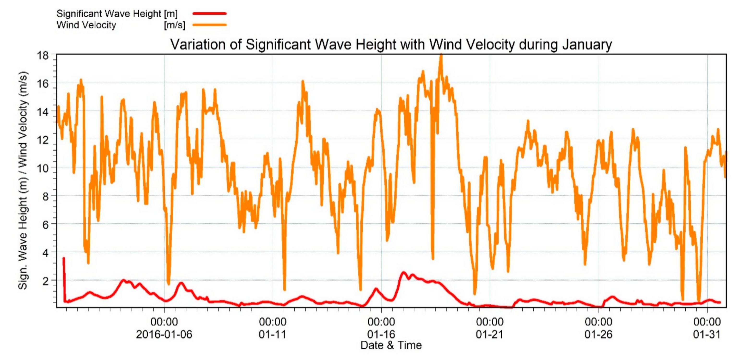
Taking into consideration that the Black Sea basin has a limited fetch, the predominant waves are the seas, with mean periods lower than 10 s [27]. In these conditions, the influence of the local winds is high, even in winter when high wind speeds are over the Black Sea basin and the possibility to find swell is higher. Thus, from Figure 12, it can be observed that the H_s variation of the waves coming near to the shore in January 2016 was consistent with the wind speed variation.

The differences between the waves encountered in the cold and warm seasons can also be understood from the calculation of the coefficient of variation. Kabiling et al. [28] presents the definition of uncertainty, or “coefficient of variation”, as:

$$\sigma {\prime }_H={\sigma }_H/H_{mean},$$

(11)

where $\sigma {\prime }_H$ represents the uncertainty for the wave height, ${\sigma }_H$ represents the standard deviation (or ‘error’), and $H_{mean}$ is the mean value of the wave height.

From the relation (11), we can see a dependence of the direct proportionality between the mean value of the significant wave height ($H_{mean}$ ) and the standard error for a given coefficient of variation (${\sigma }_H)$, so that as the height of the waves increases, its error, ${\sigma }_H$, also increases. This also applies to other wave parameters. Errors, therefore, increase with the magnitude of the waveform and decrease as their magnitude decreases.

In the Black Sea, based on the data used in this study, the coefficient of variation is 0.69, which gives us information about the high variability of the Black Sea, rather than data errors. In this area, there are large seasonal variations, where the difference between the significant summer and winter wave heights is high, and the coefficient of variation tends to be closer to 1.

Subsequently, the spectral model described above was used and some conclusions were drawn regarding the Mangalia shoreline. At the same time, the spatial and temporal changes of the wave characteristics were taken into account. These changes are morphodynamically important.

In winter, the magnitude increases for significant wave height, reaching a maximum of 2.47 m (19 February 2016), unlike the warm season reaching a maximum of 0.89 m (13 July 2016). These events prove and reinforce worrying coastal erosion cases in the winter.

5. Conclusions

Based on the results presented in this study, it can be concluded that using the MIKE 21 SW model, forced with boundary conditions provided by the SWAN model, reliable simulations of the wave conditions near to Mangalia harbor have been obtained after the calibration of the model. The wave parameters simulated by MIKE 21 SW have been compared with the measurements obtained from the MEDA buoy maintained by GeoEcoMar. The statistical parameters show a good agreement between both data.

In the Black Sea, being an enclosed sea with limited fetches, the predominant type of waves is waves that are affected by the local wind. It was observed that in winter, when the wind speeds are higher and with a high variability of the mean direction, the beach is affected by greater erosion.

During the winter months (especially in January), storms are more frequent and the wave height increases (being influenced by the changes in wind direction and wind speed) until nearly mid-spring. This leads to the formation of beach berms, shaping the beach into a more concave shape. At the same time, offshore sandbanks are formed during the winter, which subsequently help protect the beach by breaking waves off the coast.

Furthermore, during the year 2016, towards the end of the spring and during the summer and autumn months, smaller and calmer waves dominated, with the sand slowly turning back to the beach. Beaches and dunes were usually recovered if sediments were not lost at sea.