An Improved Method to Estimate the Probability of Oil Spill Contact to Environmental Resources in the Gulf of Mexico

Abstract
:1. Introduction
2. Methods
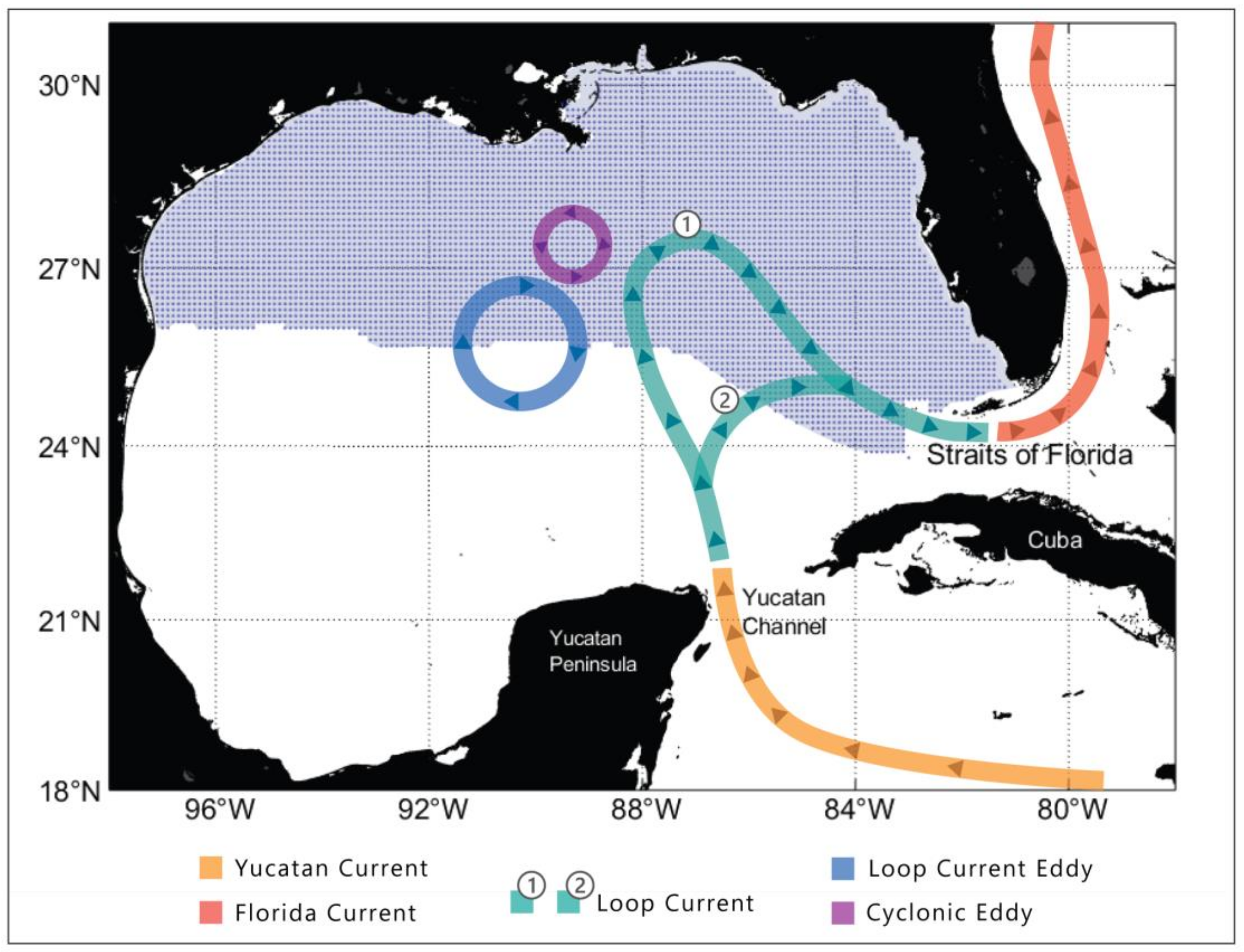
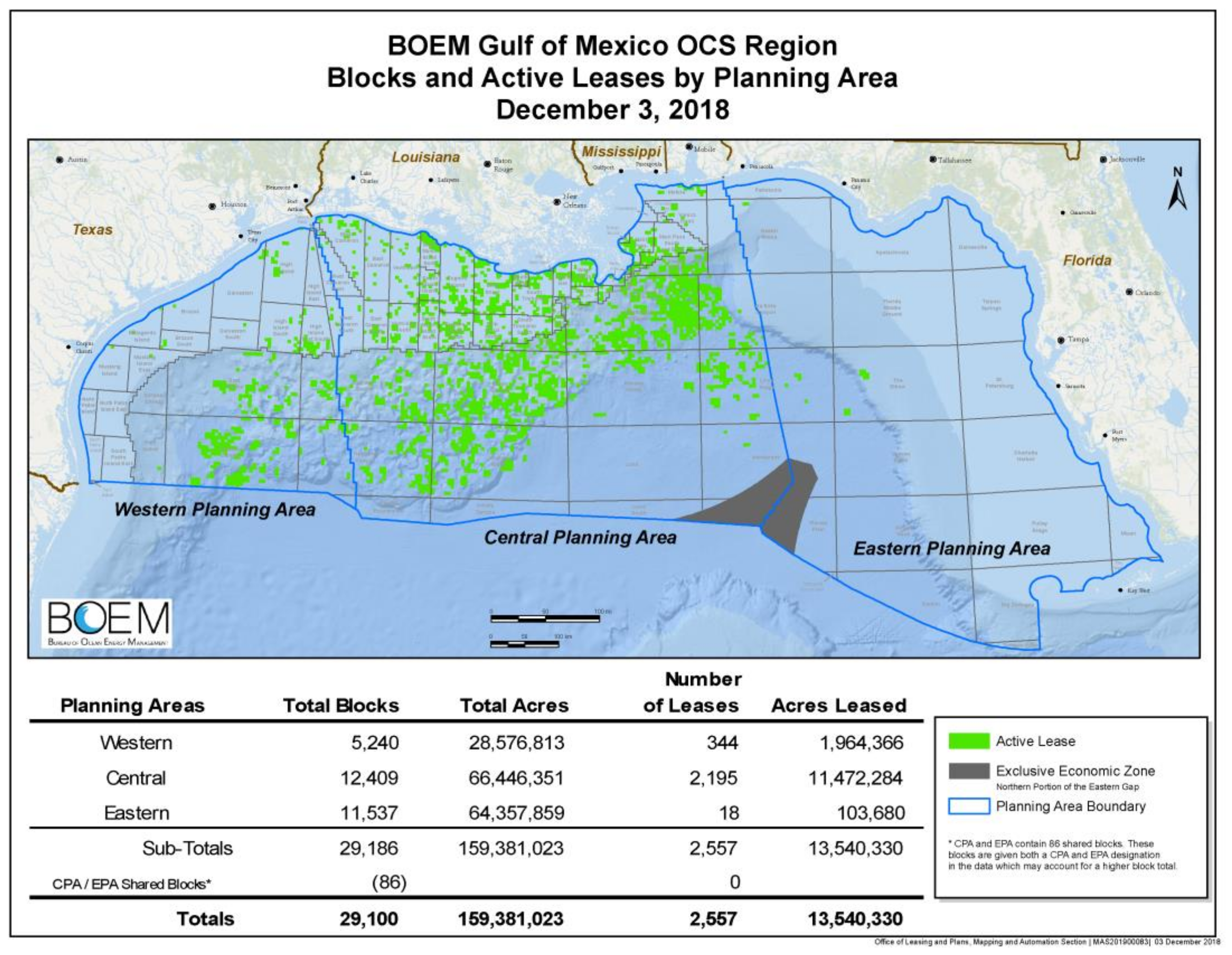
2.1. Study Area
2.2. Trajectory Simulations
2.3. Surface Wind and Ocean Current Data
2.4. Environmental Resources
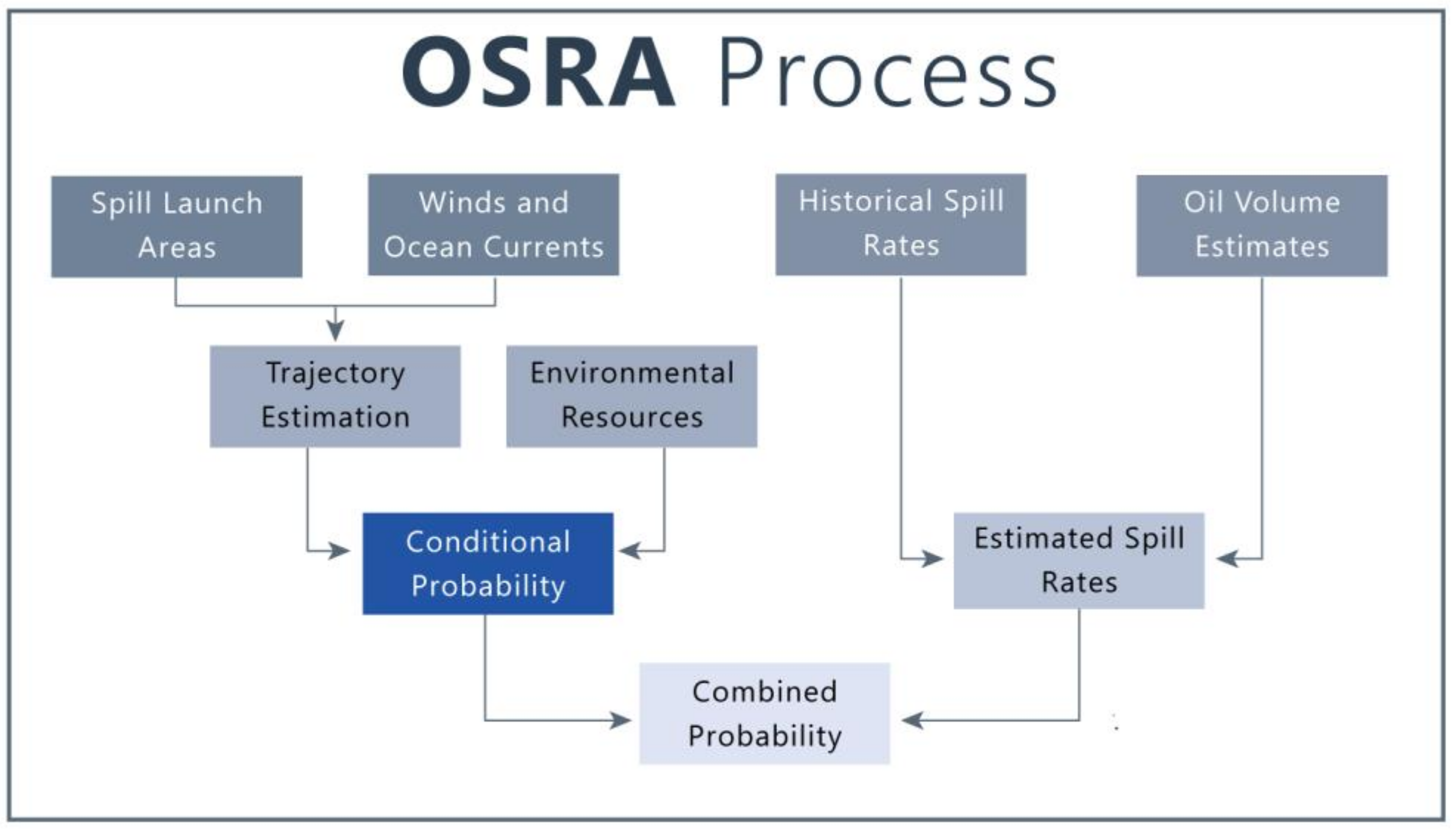
2.5. Conditional Probability
2.6. Conditional Probability from Two Launch Points in 1998
2.7. Sensitivity Studies
3. Results
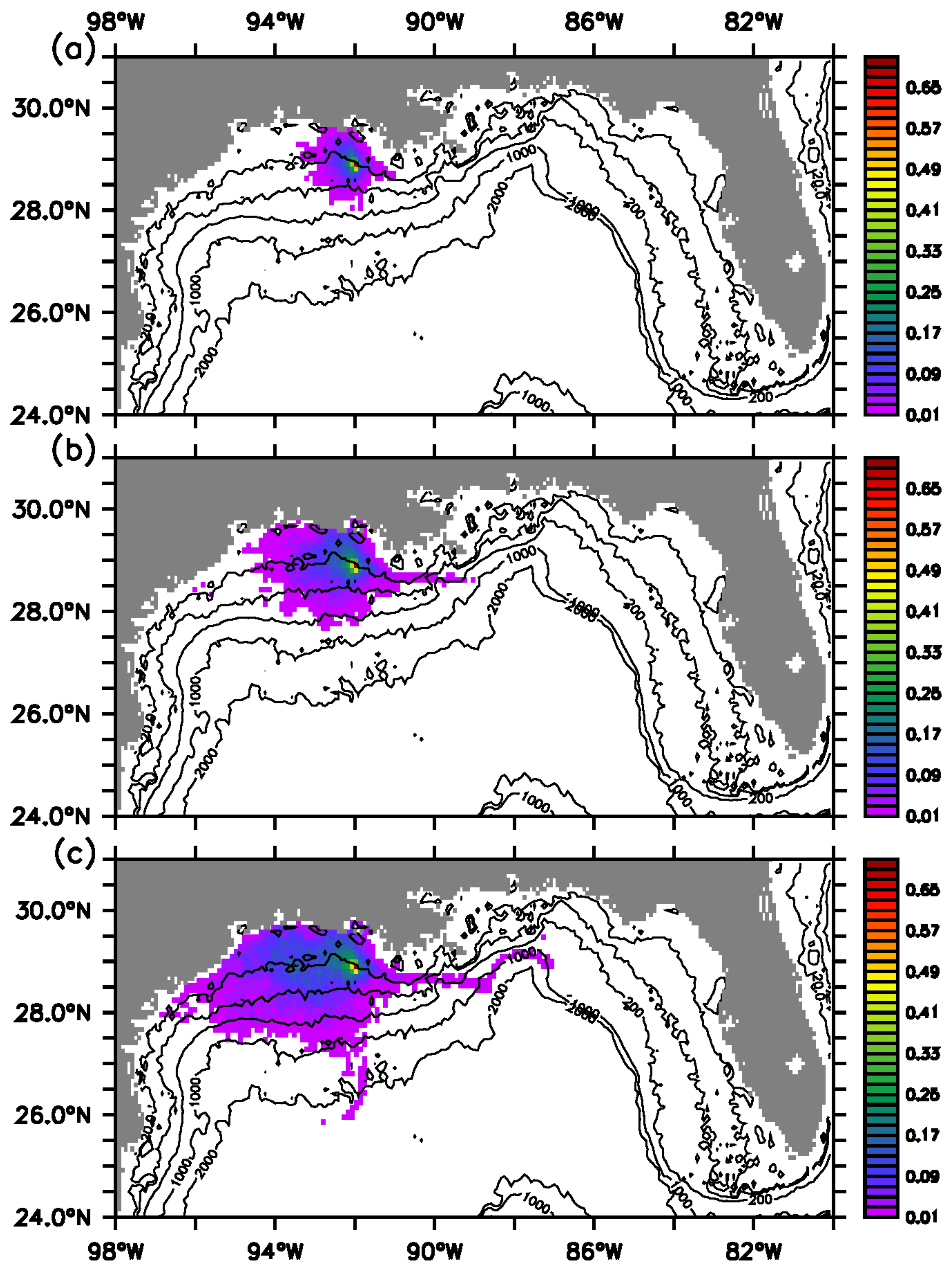
3.1. Annual Conditional Probability
3.2. Multi-Year Mean Annual Conditional Probability
3.3. Monthly Conditional Probability
3.4. Estimation of Annual Conditional Probability for a Subset of Environmental Resources
4. Discussion
Author Contributions
Funding
Acknowledgments
Conflicts of Interest
References
- Zeringue, B.A.; Yu, C.W.; Riches, T.J., Jr.; De Cort, T.M.; Maclay, D.M.; Wilson, M.G. U.S. Outer Continental Shelf Gulf of Mexico Region Oil and Gas Production Forecast: 2018–2027; OCS Report BOEM 2017–082; Department of the Interior, Bureau of Ocean Energy Management, Gulf of Mexico OCS Region: New Orleans, LA, USA, 2017; p. 32. [Google Scholar]
- Smith, R.A.; Slack, J.R.; Davis, R.K. An Oil Spill Risk Analysis for the North Atlantic Outer Continental Shelf Lease Area; Geological Survey Open-File Report 76-620; U.S. Geological Survey: Reston, VA, USA, 1976; p. 38.
- Smith, R.A.; Slack, J.R.; Wyant, T.; Lanfear, K.J. The Oilspill Risk Analysis Model of the U.S. Geological Survey; Geological Survey Professional Paper 1227; United States Government Printing Office: Washington, DC, USA, 1982; p. 40.
- LaBelle, R.P.; Samuels, W.B.; Amstutz, D.E. An Examination of the Argo Merchant Oil Spill Incident Using a Probabilistic Oil Spill Model. Presented at the 47th Annual Meeting of the American Society of Limnology and Oceanography, Vancouver, BC, Canada, 11–14 June 1984. [Google Scholar]
- Johnson, W.R.; Marshall, C.F.; Lear, E.M. Oil-Spill Risk Analysis: Pacific Outer Continental Shelf Program, Minerals Management Service; OCS Report 2000-057; OCS Report: Herndon, VA, USA, 2000; p. 290. [Google Scholar]
- Anderson, C.M.; LaBelle, R.P. Comparative Occurrence Rates for Offshore Oil Spills. Spill Sci. Technol. Bull. 1994, 1, 131–141. [Google Scholar] [CrossRef]
- Anderson, C.M.; LaBelle, R.P. Update of Comparative Occurrence Rates for Offshore Oil Spills. Spill Sci. Technol. Bull. 2000, 6, 303–321. [Google Scholar] [CrossRef]
- Anderson, C.M.; Mayes, M.; LaBelle, R.P. Update of Occurrence Rates for Offshore Oil Spills; OCS Report 2012-069; Bureau of Ocean Energy Management Division of Environmental Assessment, and Bureau of Safety and Environmental Enforcement: Herndon, VA, USA, 2012. Available online: http://www.boem.gov/uploadedFiles/BOEM/Environmental_Stewardship/Environmental_Assessment/Oil_Spill_Modeling/AndersonMayesLabelle2012.pdf (accessed on 21 December 2018).
- Price, J.M.; Johnson, W.R.; Marshall, C.F.; Ji, Z.-G.; Rainey, G.B. Overview of the Oil Spill Risk Analysis (OSRA) Model for Environmental Impact Assessment. Spill Sci. Technol. Bull. 2003, 8, 529–533. [Google Scholar] [CrossRef]
- Price, J.M.; Johnson, W.R.; Ji, Z.-G.; Marshall, C.F.; Rainey, G.B. Sensitivity Testing for Improved Efficiency of a Statistical Oil-Spill Risk Analysis Model. Environ. Model. Softw. 2004, 19, 671–679. [Google Scholar] [CrossRef]
- Guillen, G.; Rainey, G.; Morin, M. A Simple Rapid Approach Using Coupled Multivariate Statistical Methods, GIS and Trajectory Models to Delineate Areas of Common Oil Spill Risk. J. Mar. Syst. 2004, 45, 221–235. [Google Scholar] [CrossRef]
- Ji, Z.-G.; Johnson, W.R.; Li, Z.; Green, R.E.; O’Reilly, S.E.; Gravois, M.P. Oil-Spill Risk Analysis: Gulf of Mexico Outer Continental Shelf (OCS) Lease Sales, Eastern Planning Area, 2012–2017, and Eastern Planning Area OCS Program, 2012–2051; OCS Report BOEM 2013–0110; Department of the Interior, Bureau of Ocean Energy Management: Herndon, VA, USA, 2013; p. 61.
- Johnson, W.R.; Ji, Z.-G.; Marshall, C.F. Statistical Estimates of Shoreline Oil Contact in the Gulf of Mexico. In Proceedings of the International Oil Spill Conference, Miami Beach, FL, USA, 15–19 May 2005; pp. 547–551. [Google Scholar]
- Lugo-Fernandez, A.; Morin, M.V.; Ebesmeyer, C.C.; Marshall, C.F. Gulf of Mexico Historic (1955–1987) Surface Drifter Data Analysis. J. Coast. Res. 2001, 17, 1–6. [Google Scholar]
- Price, J.M.; Reed, M.; Howard, M.K.; Johnson, W.R.; Ji, Z.-G.; Marshall, C.F.; Guinasso, C.N., Jr.; Rainey, G.B. Preliminary Assessment of an Oil-Spill Trajectory Model using Satellite-Tracked, Oil-Spill-Simulating Drifters. Environ. Model. Softw. 2006, 21, 258–270. [Google Scholar] [CrossRef]
- Ji, Z.-G.; Johnson, W.R.; Li, Z. Oil Spill Risk Analysis Model and its Application to the Deepwater Horizon Oil Spill Using Historical Current and Wind data. In Monitoring and Modeling the Deepwater Horizon Oil Spill: A Record-Breaking Enterprise; Liu, Y., MacFadyen, A., Ji, Z.-G., Weisberg, R.H., Eds.; American Geophysical Union: Washington, DC, USA, 2011; pp. 227–236. [Google Scholar]
- Zheng, L.; Yapa, P.D.; Chen, F.H. A Model for Simulating Deepwater Oil and Gas Blowouts—Part I: Theory and Model Formulation. J. Hydraul. Res. 2003, 41, 339–351. [Google Scholar] [CrossRef]
- Chen, F.; Yapa, P.D. A Model for Simulating Deep Water Oil and Gas Blowouts—Part II: Comparison of Numerical Simulations with “Deepspill” Field Experiments. J. Hydraul. Res. 2003, 41, 353–365. [Google Scholar] [CrossRef]
- Yapa, P.D.; Chen, F.H. Behavior of Oil and Gas from Deepwater Blowouts. J. Hydraul. Res. 2004, 130, 540–553. [Google Scholar] [CrossRef]
- LaBelle, R.P.; Lane, J.S. Meeting the Challenge of Deepwater Spill Response. In Proceedings of the International Oil Spill Conference, Tampa, FL, USA, 26–29 March 2001; pp. 705–708. [Google Scholar]
- LaBelle, R.P. Overview of US Minerals Management Service Activities in Deepwater Research. Mar. Pollut. Bull. 2001, 43, 256–261. [Google Scholar] [CrossRef]
- Beegle-Krause, C.J. General NOAA Oil Modeling Environment (GNOME): A New Spill Trajectory Model. In Proceedings of the International Oil Spill Conference, Tampa, FL, USA, 26–29 March 2001; pp. 865–871. [Google Scholar]
- MacFadyen, A.; Watabayashi, G.Y.; Barker, C.H.; Beegle-Krause, C.J. Tactical Modeling of Surface Oil Transport during the Deepwater Horizon Spill Response. In Monitoring and Modeling the Deepwater Horizon Oil Spill: A Record-Breaking Enterprise; Liu, Y., MacFadyen, A., Ji, Z.-G., Weisberg, R.H., Eds.; American Geophysical Union: Washington, DC, USA, 2011; pp. 167–178. [Google Scholar]
- Reed, M.; Singsaas, I.; Daling, P.S.; Faksness, L.-G.; Brakstad, O.G.; Hetland, B.A.; Hokstad, J.N. Modeling the Water-accommodated Fraction in OSCAR2000. In Proceedings of the International Oil Spill Conference, Tampa, FL, USA, 26–29 March 2001; pp. 1083–1091. [Google Scholar]
- Oey, L.-Y.; Lee, H.-C. Deep Eddy Energy and Topographic Rossby Waves in the Gulf of Mexico. J. Phys. Oceanogr. 2002, 32, 3499–3527. [Google Scholar] [CrossRef]
- Oey, L.-Y.; Lee, H.-C.; Schmitz, W.J., Jr. Effects of Winds and Caribbean Eddies on the Frequency of Loop Current Eddy Shedding: A Numerical Model Study. J. Geophys. Res. 2003, 108, 3324. [Google Scholar] [CrossRef]
- Oey, L.-Y. Circulation Model of the Gulf of Mexico and the Caribbean Sea: Development of the Princeton Regional Ocean Forecast (& Hindcast) System–PROFS, and Hindcast Experiment for 1992–1999; OCS Study MMS 2005–049, Final Report; Department of the Interior, Minerals Management Service: Herndon, VA, USA, 2005; p. 174. [Google Scholar]
- Chang, Y.-L.; Oey, L.; Xu, F.-H.; Lu, H.-F.; Fujisaki, A. Oil spill: Trajectory Projections Based on Ensemble Drifter Analyses. Ocean Dyn. 2011, 61, 829–839. [Google Scholar] [CrossRef]
- Wang, D.-P.; Oey, L.-Y.; Ezer, T.; Hamilton, P. Near-Surface Currents in DeSoto Canyon (1997–1999): Comparison of Current Meters, Satellite Observations, and Model Simulation. J. Phys. Oceanogr. 2003, 33, 313–326. [Google Scholar] [CrossRef]
- Ezer, T.; Oey, L.-Y.; Lee, H.-C.; Sturges, W. The Variability of Currents in the Yucatan Channel: Analysis of Results from a Numerical Ocean Model. J. Geophys. Res. 2003. [Google Scholar] [CrossRef]
- Fan, S.J.; Oey, L.-Y.; Hamilton, P. Assimilation of Drifter and Satellite Data in a Model of the Northeastern Gulf of Mexico. Cont. Shelf Res. 2004, 24, 1001–1013. [Google Scholar] [CrossRef]
- Oey, L.-Y.; Ezer, T.; Lee, H.-C. Loop Current, Rings and Related Circulation in the Gulf of Mexico: A Review of Numerical Models and Future Challenges. In Circulation in the Gulf of Mexico: Observations and Models; Geophysical Union Geophysical Monograph Series; Wiley: Hoboken, NJ, USA, 2005; Volume 161, pp. 32–56. [Google Scholar]
- Oey, L.-Y.; Ezer, T.; Forristall, G.; Cooper, C.; DiMarco, S.; Fan, S. An Exercise in Forecasting Loop Current and Eddy Frontal Positions in the Gulf of Mexico. Geophys. Res. Lett. 2005, 32, L12611. [Google Scholar] [CrossRef]
- Oey, L.-Y.; Ezer, T.; Wang, D.-P.; Fan, S.; Yin, X.-Q. Loop Current Warming by Hurricane Wilma. Geophys. Res. Lett. 2006, 33, L08613. [Google Scholar] [CrossRef]
- Oey, L.-Y.; Ezer, T.; Wang, D.-P.; Yin, X.-Q.; Fan, S.-J. Hurricane-induced Motions and Interaction with Ocean Currents. Cont. Shelf Res. 2007, 27, 1249–1263. [Google Scholar] [CrossRef]
- Oey, L.-Y.; Inoue, M.; Lai, R.; Lin, X.-H.; Welsh, S.; Rouse, L., Jr. Stalling of Near-inertial Waves in a Cyclone. Geophys. Res Lett. 2008, 35, L12604. [Google Scholar] [CrossRef]
- Oey, L.-Y. Loop Current and Deep Eddies. J. Phys. Oceanogr. 2008, 38, 1426–1449. [Google Scholar] [CrossRef]
- Oey, L.-Y.; Chang, Y.-L.; Sun, Z.-B.; Lin, X.-H. Topocaustics. Ocean Model. 2009, 29, 277–286. [Google Scholar] [CrossRef]
- Yin, X.-Q.; Oey, L.-Y. Bred-ensemble Ocean Forecast of Loop Current and Rings. Ocean Model. 2007. [Google Scholar] [CrossRef]
- Lin, X.-H.; Oey, L.-Y.; Wang, D.-P. Altimetry and Drifter Data Assimilations of Loop Current and Eddies. J. Geophys. Res. 2007, 112, C05046. [Google Scholar] [CrossRef]
- Barker, C.H. A Statistical Outlook for the Deepwater Horizon Oil Spill. In Monitoring and Modeling the Deepwater Horizon Oil Spill: A Record-Breaking Enterprise; Liu, Y., MacFadyen, A., Ji, Z.-G., Weisberg, R.H., Eds.; American Geophysical Union: Washington, DC, USA, 2011; pp. 237–244. [Google Scholar]
- Alves, T.M.; Kokinou, E.; Zodiatis, G.A. Three-step Model to Assess Shoreline and Offshore Susceptibility to Oil Spills: The South Aegean (Crete) as an Analogue for Confined Marine Basins. Mar. Pollut. Bull. 2014, 86, 443–457. [Google Scholar] [CrossRef] [PubMed]
- Alves, T.M.; Kokinou, E.; Zodiatis, G.A.; Lardner, R.; Panagiotakis, C.; Radhakrishnan, H. Modelling of Oil Spills in Confined Maritime Basins: The Case for Early Response in the Eastern Mediterranean Sea. Environ. Pollut. 2015, 206, 390–399. [Google Scholar] [CrossRef]
- Alves, T.M.; Kokinou, E.; Zodiatis, G.A.; Radhakrishnan, H.; Panagiotakis, C.; Lardner, R. Multidisciplinary Oil Spill Modeling to Protect Coastal Communities and the Environment of the Eastern Mediterranean Sea. Sci. Rep. 2016, 6. [Google Scholar] [CrossRef]
- Forristal, G.Z.; Schaudt, K.J.; Cooper, C.K. Evolution and Kinematics of a Loop Current Eddy in the Gulf of Mexico during 1985. J. Geophys. Res. 1992, 97, 2173–2184. [Google Scholar] [CrossRef]
- Sturges, W.; Leben, R. Frequency of Ring Separations from the Loop Current in the Gulf of Mexico: A Revised Estimate. J. Phys. Oceanogr. 2000, 30, 1814–1819. [Google Scholar] [CrossRef]
- Sturges, W.; Lugo-Fernandez, A. (Eds.) Circulation in the Gulf of Mexico: Observations and Models; Geophysical Monograph Series; American Geophysical Union: Washington, DC, USA, 2005; Volume 161, p. 347. [Google Scholar]
- Samuels, W.B.; Huang, N.E.; Amstutz, D.E. An Oilspill Trajectory Analysis Model with a Variable Wind Deflection Angle. Ocean Eng. 1982, 9, 347–360. [Google Scholar] [CrossRef]
- Department of the Interior, Bureau of Ocean Energy Management. Gulf of Mexico OCS oil and Gas Lease Sales: 2014 and 2016; Eastern Planning Area Lease Sales 225 and 226—Final Environmental Impact Statement; OCS EIS/EA BOEM 2013-200; Department of the Interior, Bureau of Ocean Energy Management, Gulf of Mexico Region: New Orleans, LA, USA, 2013; Volume 1.
- Oey, L.-Y. Extended Hindcast Calculation of Gulf of Mexico Circulation: Model Development, Comparison with Observations, and Application to the 2010 Oil Spill. Unpublished work.
- Mellor, G.L. User Guide for a Three-Dimensional, Primitive Equation, Numerical Ocean Model (Jul/2002 Version); Program in Atmospheric and Oceanic Sciences, Princeton University: Princeton, NJ, USA, 2002; p. 42. Available online: http://www.ccpo.odu.edu/POMWEB/UG.10-2002.pdf (accessed on 21 December 2018).
- Adler, E.; Inbar, M. Shoreline Sensitivity to Oil Spills, the Mediterranean Coast of Israel:Assessment and Analysis. Ocean Coast. Manag. 2007, 50, 24–34. [Google Scholar] [CrossRef]
- Yang, H.; Weisberg, R.H.; Niiler, P.P.; Sturges, W.; Johnson, W. Lagrangian Circulation and Forbidden Zone on the West Florida Shelf. Cont. Shelf Res. 1999, 19, 1221–1245. [Google Scholar] [CrossRef]
- Sturges, W.; Niiler, P.P.; Weisberg, R.H. Northeastern Gulf of Mexico Inner Shelf Circulation Study; Final Report, MMS Cooperative Agreement 14-35-0001-30787, OCS Report MMS 2001–103; US Minerals Management Service: Herndon, VA, USA, 2001; p. 90.
- Nowlin, W.D., Jr.; Jochens, A.E.; DiMarco, S.F.; Reid, R.O.; Howard, M.K. Low-frequency Circulation over the Texas-Louisiana Continental Shelf. In Circulation in the Gulf of Mexico: Observations and Models; Geophysical Monograph Series; Sturges, W., Lugo-Fernandez, A., Eds.; American Geophysical Union: Washington, DC, USA, 2005; Volume 161, pp. 219–240. [Google Scholar]
- Johansen, O.; Rye, H.; Cooper, C. DeepSpill—Field Study of a Simulated Oil and Gas Blowout in Deep Water. Spill Sci. Technol. Bull. 2003, 8, 433–443. [Google Scholar] [CrossRef]
- Chelton, D.B.; de Szoeke, R.A.; Schlax, M.G.; El Naggar, K.; Siwertz, N. Geographical Variability of the First Baroclinic Rossby Radius of Deformation. J. Phys. Oceanogr. 1998, 28, 433–460. [Google Scholar] [CrossRef]


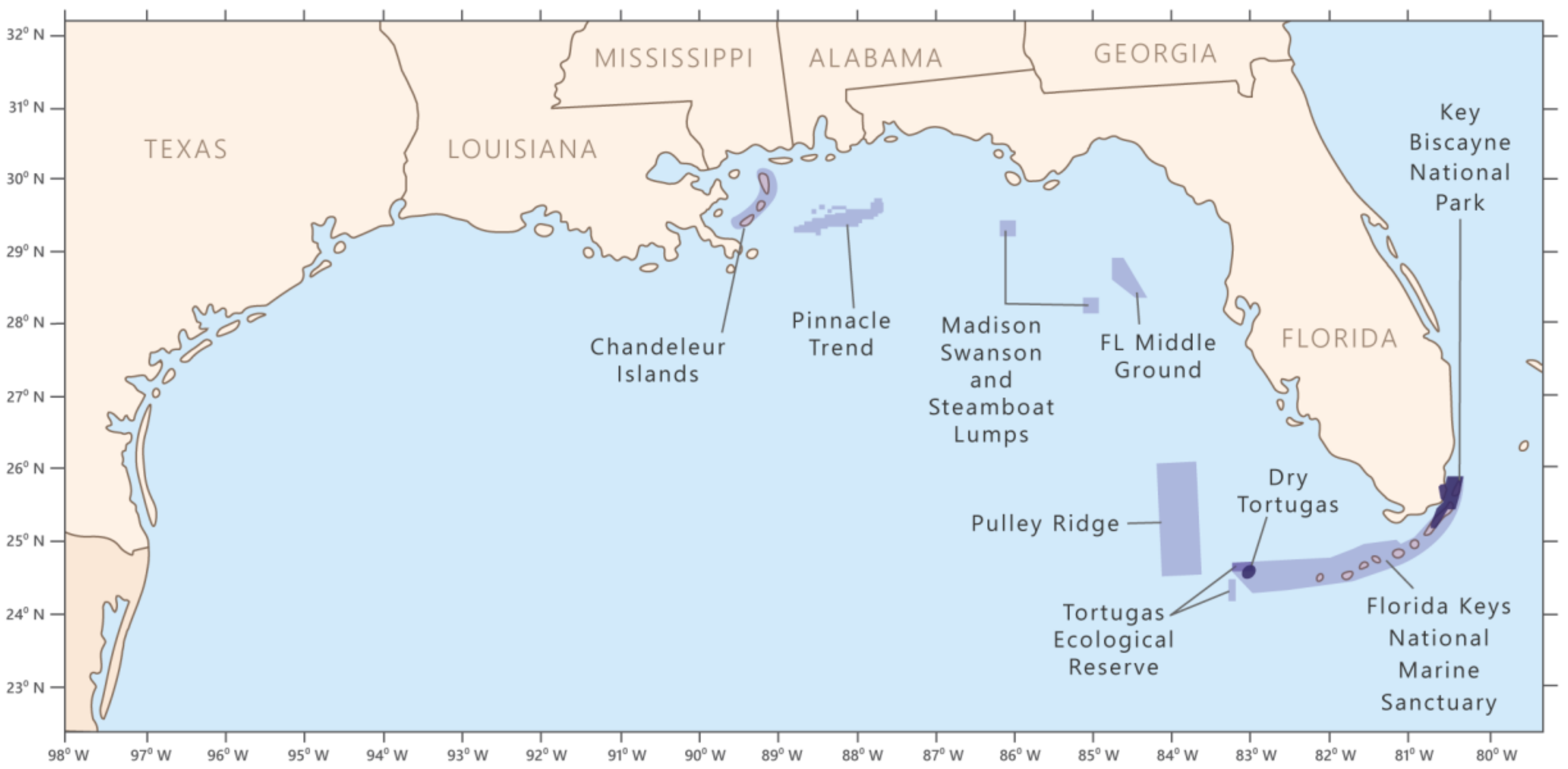
| Environmental Resource | 1993–1998 | 2000–2006 | ||
|---|---|---|---|---|
| Mean | SD | Mean | SD | |
| Chandeleur Islands | 0.0061 | 0.0009 | 0.0054 | 0.0010 |
| Madison Swanson and Steamboat Lumps Marine Reserve | 0.0100 | 0.0009 | 0.0084 | 0.0005 |
| Florida Middle Ground | 0.0084 | 0.0008 | 0.0072 | 0.0007 |
| Pulley Ridge | 0.0123 | 0.0022 | 0.0118 | 0.0017 |
| Pinnacle Trend | 0.0107 | 0.0008 | 0.0098 | 0.0013 |
| Tortugas Ecological Reserve (North & South) | 0.0178 | 0.0050 | 0.0143 | 0.0031 |
| Key Biscayne National Park | 0.0088 | 0.0018 | 0.0061 | 0.0011 |
| Dry Tortugas | 0.0100 | 0.0009 | 0.0090 | 0.0011 |
| Florida Keys National Marine Sanctuary | 0.0112 | 0.0015 | 0.0093 | 0.0014 1 |
© 2019 by the authors. Licensee MDPI, Basel, Switzerland. This article is an open access article distributed under the terms and conditions of the Creative Commons Attribution (CC BY) license (http://creativecommons.org/licenses/by/4.0/).
Share and Cite
Li, Z.; Johnson, W. An Improved Method to Estimate the Probability of Oil Spill Contact to Environmental Resources in the Gulf of Mexico. J. Mar. Sci. Eng. 2019, 7, 41. https://doi.org/10.3390/jmse7020041
Li Z, Johnson W. An Improved Method to Estimate the Probability of Oil Spill Contact to Environmental Resources in the Gulf of Mexico. Journal of Marine Science and Engineering. 2019; 7(2):41. https://doi.org/10.3390/jmse7020041
Chicago/Turabian StyleLi, Zhen, and Walter Johnson. 2019. "An Improved Method to Estimate the Probability of Oil Spill Contact to Environmental Resources in the Gulf of Mexico" Journal of Marine Science and Engineering 7, no. 2: 41. https://doi.org/10.3390/jmse7020041