Rogue Wave Formation in Adverse Ocean Current Gradients

Abstract

Studies of the nonlinear Schrödinger (NLS) equation indicate that surface gravity waves traveling against currents of increasing strength gain energy and steepness in the process, and this can be a mechanism for rogue wave formation. Likewise, experimental studies have shown that stable wavetrains traveling against adverse currents can give rise to extreme waves. We studied this phenomenon by using computational fluid dynamics (CFD) tools, whereby the non-hydrostatic Euler equations were solved utilizing the finite volume method. Waveforms based on a JONSWAP spectrum were generated in a numerical wave tank and were made to travel against current gradients of known strength, and wave characteristics were monitored in the process. We verified that waves gain energy from the underlying flow field as they travel against current gradients, and the simulated level of energy increase was comparable to that predicted by earlier studies of the NLS equation. The computed significant wave height, $H_s$, increased substantially, and there were strong indications that the current gradients induced nonlinear wave instabilities. The simulations were used to determine a new empirical relationship that correlates changes in the current velocity to changes in the Benjamin–Feir Index (BFI). The empirical relationship allows for seafaring entities to predict increased risk of rogue waves ahead, based on wave and current conditions.

1. Introduction

Rogue waves and the candidate physical mechanisms that can give rise to them have been studied analytically, numerically, and experimentally. Benjamin and Feir [1] described the modulational instability, whereby two spectral sidebands get amplified via energy transfer from a central frequency-carrier wave. A rogue, or freak, wave is defined as a wave that is at least as high as twice the significant wave height, $H_{rogue}\ge 2H_s$. Significant wave height, $H_s$, is defined as the average of the highest one-third of waves. A review of the physical mechanisms that can cause rogue waves to appear can be found in [2,3], but, in general, they fall under the two broad categories of linear and nonlinear wave theory. Linear theory predicts the genesis of rogue waves by linear superposition, or focusing, of wave groups—spatiotemporal in 2D waves and spatial (geometric) in 3D waves. It also predicts rogue waves appearing from the interaction of waves with currents that are sufficiently strong to cause blocking. This is essentially the scenario of an extreme Doppler shift caused by a current that is strong enough to induce wave focusing at the blocking point. Nonlinear theory accounts for the energy transfer between interacting spectral components and includes the phenomenon of self-modulation; the modulational instability is the most widely studied nonlinear interaction, and its action in water waves has been demonstrated experimentally [4,5,6]. Its significance as a rogue wave-generating mechanism in the ocean is still unclear, however, because its action is known to weaken substantially with increased wave directionality [7,8,9]. Nonlinear wave interactions as physical phenomena that can potentially generate rogue waves in the ocean remain a topic of active research [10]. A family of modern numerical models/tools that are founded on dispersive partial differential equations (PDEs) has been developed by the scientific community to study such phenomena. A concise overview on the topic can be found in [3]. The nonlinear Schrödinger (NLS) equation is one of the equations in this family of PDEs, whose members are able to capture nonlinear wave interactions and freak wave formation in a diverse array of dispersive media, ranging from the ocean to optical fibers [11].

A general, widely accepted rule is that wave conditions characterized by steep power spectra, where energy is concentrated in a narrow bandwidth, are more prone to give birth to rogue waves as the product of nonlinear interactions and concomitant rapid energy exchange between spectral components and wave height buildup [2]. This conclusion/result is also derived in mathematical models that make use of dispersive PDEs [3]. From a conceptual perspective, and with reference to perturbation theory, energy concentration over a narrow bandwidth translates into increased steepness of the waves in that bandwidth, and the latter parameter is directly correlated to the level of nonlinear behavior of the system [12]. The standard metric for assessing the risk of rogue wave appearance in random sea states is the Benjamin–Feir Index (BFI), given as [13]:

$$BFI=\frac{\sqrt{2}{k}_p{H}_s}{4{\sigma }_{\omega }^{\prime }},$$

(1)

where $k_p$ is the peak wavenumber of the spectrum, and where ${\sigma }_{\omega }^{\prime }$ is the bandwidth, $\Delta \omega$, normalized by the peak angular frequency, ${\omega }_p$. The ratio $\frac{1}{{\sigma }_{\omega }^{\prime }}$ is a measure of spectral ‘peakedness’ or narrowness, with higher values signifying energy concentration in a narrow bandwidth, while $H_s$ is a measure of total spectral energy, E, and is related to the latter by $H_s\approx 4\sqrt{E}$. The BFI was first proposed by Janssen [10], who derived it from the Zakharov equation [14], but a similar formulation was also given by Onorato et al. [15]. BFI values greater than unity indicate a higher risk for a rogue wave incident. Wave conditions such as these are also characterized by wave height probability distributions that deviate from the Gaussian norm with respect to the probability of unusually high waves. The statistical metric most relevant to measuring such deviations is kurtosis or ‘tailedness’, $\kappa$, which involves the probability distribution of the surface elevation, $\eta$. The tailedness $\kappa$ is defined as the ratio of the fourth to the square of the second-order moment of $\eta$, $\frac{<{\eta }^4>}{{(<{\eta }^2>)}^2}$. The wave height distribution in the ocean is normally Gaussian, with kurtosis values close to 3. Under such conditions, rogue waves have approximately a ${10}^{-4}$ probability of appearing. Higher kurtosis values mark a departure from Gaussian statistics and a higher probability of freak wave appearance resulting from nonlinear wave interactions. The kurtosis may be expressed in terms of the BFI as [16]:

$$\kappa =3+\frac{\pi }{\sqrt{3}}BF{I}^2.$$

(2)

Adverse current gradients can induce the Benjamin–Feir instability in the ocean, and it has been known for a long time that the region of the Agulhas current, which flows from the north-east off the southeast coast of Africa and collides with winds from the south-west, is an area where huge rogue waves appear. Several large ships have been severely damaged or sunk by rogue waves in that area, and, in some cases, tens of people lost their lives [17]. Adverse current gradients increase the value of the BFI in several ways; they induce a transfer of energy from the flow field to overlying waves, thus increasing the value of $H_s$. Moreover, the transfer of energy is such that higher waves gain more energy [18,19], which causes spectral energy to increase over a narrow bandwidth, and spectral narrowness to increase as well. In addition, wavelength shortening due to the Doppler shift causes wave steepness and $k_p$ to increase.

Rogue waves have been produced in wave tanks by triggering the modulational instability under the action of adverse current gradients [20,21,22]. Another study tested short-crested wave formations in a directional wave tank under the action of current gradients [23] and found that current gradients, despite wave directionality, induced increases in kurtosis, raising the probability of rogue wave appearance.

The effects of adverse current gradients on waves have been studied numerically by making use of the NLS equation [12,18,19,24]. The studies indicate that wave formations traveling in nonuniform currents are subject to an energy transformation that induces instabilities. It is worth noting that some types of the interactions simulated by solving the NLS have recently been observed as commonly occurring in nature, as in the case of X- and Y-type interactions between solitons in shallow water under the action of tidal currents [25]. The NLS modified for the presence of a current, in the form that is most relevant to our study, was derived by Hjelmervik and Trulsen [12] from the Euler equations by making use of perturbation theory. Historically, a modified cubic Schrödinger equation (MCSE) was derived earlier by Gerber [26], who accounted for various scenarios of wave–current interactions in his analytical study. Onorato et al. [18] proposed a modification to the NLS [12] for nonuniform currents and provided an analytical estimate for the increase in energy of waves traveling against a current gradient1. Specifically, on the basis of their study, a wave envelope of some general form traveling a distance $\Delta x=x-x_o$ against a current of increasing strength, $|\Delta U|=|U(x)-U_{(xo)}|$, will gain an amount of energy from the underlying flow field given by [18,22]:

$$E=E_{o}exp(\frac{-2\Delta U}{c_g}),$$

(3)

where $E_o$ is the initial energy level (at $x_o$), and $c_g$ is the group velocity or, more precisely, half the ’characteristic’ or phase velocity, $c_p$, in deep water. The result is significant because it provides a quantitative estimate of the changes in the characteristics of waves traveling in nonuniform currents. Furthermore, these changes become noticeable at relatively weak current strengths. The two main provisions for the analysis leading to Equation (3) are that the current strength, $\left|U\right|$, is relatively small ($\mathcal{O}(|U/c_g|)={10}^{-1}$) and that the current strength varies gradually compared with wavelength values. The phenomenon of wave amplitude increase under the action of nonuniform currents can be derived from linear theory, as presented by Ruban [19]. Ardhuin et al. [27] applied linear theory to estimate variations in $H_s$ due to wave–current interactions in the ocean on the basis of realistic directional wave spectra and current profiles. It was concluded that currents play an important role at smaller scales (<100 km) in affecting $H_s$ in the open ocean. A recent study based on field observations from two experiments confirmed that currents act locally in the open ocean to induce sharp variations in $H_s$ [28]. The study demonstrated abrupt variations in wave patterns at scales <1 km, induced by current variations in directional sea states, and it also showed the appearance of rogue waves.

While studies of the NLS rest on higher-order theory, our objective is to study the effect of currents on waves by solving the full equations of fluid motion on the basis of a continuum mechanics approach. We used computational fluid dynamics (CFD) software to study the energy evolution of random waves comprising JONSWAP-like spectra traveling against currents of gradually increasing strength. We studied wave growth as a function of increments in current strength, and wave characteristics were chosen so that wave breaking was avoided. We monitored wave spectral energy increase as waves traveled against current gradients of varying characteristics, and we compared our results with theory (Equation (3)). Wave and current characteristics were chosen so that the ratio $|\frac{\Delta U}{c_g}|$ governing wave-energy increase would be comparable in magnitude to values commonly found in oceanic zones with currents. To the best of our knowledge, this marks the first time that a CFD tool is utilized to simulate the gradual spectral energy increase and wave growth of random waves under the influence of adverse current gradients, where parameters are chosen so that ocean conditions are realistically reproduced.

This paper is organized as follows: In Section 2, we provide some information on the CFD model that we used in our study. In Section 3, we describe grid resolution and the convergence study that we carried out, as well as our model setup, i.e., important parameters and values characterizing the numerical wave tank, the wavemaker, and the currents that are implemented. In Section 4, we present our findings and the steps that we took to reach them, followed by a discussion of our results and concluding remarks in Section 5. In Appendix A, we provide information on the methodology that we followed to account for the problem of numerical energy dissipation in our simulations and to calibrate our model accordingly.

2. The CFD Model

The model that we used in our work was the non-hydrostatic wave model (NHWAVE) [29], which is configured to solve the fully 3D, non-hydrostatic, Navier–Stokes (N–S) equations. A sigma coordinate is implemented for following the terrain, as well as the free surface. Several options are provided to solve for diffusion in the N–S equations, but we chose to treat the problem as inviscid, as waves of small steepness were used, and no wave breaking took place in any of our simulations. In effect, the non-hydrostatic Euler equations were solved by NHWAVE in our simulations, which, after applying the Boussinesq approximation, are presented in conservative form as:

$$\nabla ·\rho \mathbf{u}=0$$

(4)

$$\frac{\partial \rho \mathbf{u}}{\partial t}+\nabla ·(\rho \mathbf{u}\otimes \mathbf{u}+(p_h+p_{nh})\mathbf{I})=0.$$

(5)

where $\mathbf{u}$ is the velocity vector, $\rho$ is density, $\mathbf{I}$ is the identity tensor, and where the pressure has been decomposed into a hydrostatic component, $p_h$, and a non-hydrostatic component, $p_{nh}$.

The solution algorithm proceeds on the basis of a two-stage, second-order, Runge–Kutta time-stepping scheme. Momentum fluxes through cell faces are computed by utilizing a second-order, Godunov-type, monotonicity-preserving (total variation diminishing) scheme. In the 1D case, the velocity, u, inside cell i is reconstructed in a piecewise linear manner on the basis of its value at the cell center, $u_i$, as:

$$u=u_i+(x-x_i)\frac{\Delta u}{\Delta x}.$$

(6)

The van Leer limiter [30] is used to compute the gradient, $\frac{\Delta u}{\Delta x}$. To compute the fluxes through each side, $i\pm \frac{1}{2}$, the Harten–Lax–van Leer (HLL) scheme [31] is implemented. Further details on the exact mathematical expressions can be found in Ma et al. [29].

The model has been previously validated through a series of studies, including solitary wave propagation, wave shoaling in the case of varying bed geometry, as well as wave breaking [29,32]. Computationally, adaptive time-stepping on the basis of the Courant–Friedrichs–Lewy (CFL) criterion enables faster run times, while the Poisson equation is solved by utilizing the highly efficient HYPRE library, and the code is parallelized using the message passing interface (MPI). The above characteristics, combined with the second-order spatial and temporal accuracy, make the model suitable for use in simulations of waves in large domains. Furthermore, as we explain in Section 3.1, the boundary conditions in the model can be adjusted to allow for concurrent implementation of currents of varying characteristics in addition to a wavemaker. It is this capability that allowed us to study waves traveling in nonuniform currents.

3. Methodology

The objective of this study is to simulate the gradual evolution of random waves traveling several kilometers in the ocean against currents of increasing strength. Equation (3) is derived with no a priori assumptions about initial wave characteristics. The waves that were produced by the wavemaker were mild, with steepness values below 0.1, which prevented any wave breaking from taking place, as we wanted to isolate and study the phenomenon of wave-energy gain and wave growth induced by the current gradient. For the domain length that we implemented in our simulations (≈5 km), natural dissipation could be neglected and the flow treated as inviscid, since it is known that swells can travel thousands of kilometers before losing their energy [33]. We limited our study to 2D simulations, as running 3D simulations proved to be prohibitively expensive computationally: each of our 2D simulations required a minimum of approximately 10,000 cpu hours, and the number of cores available to us placed 3D simulations out of reach with respect to the timeframe of the project.

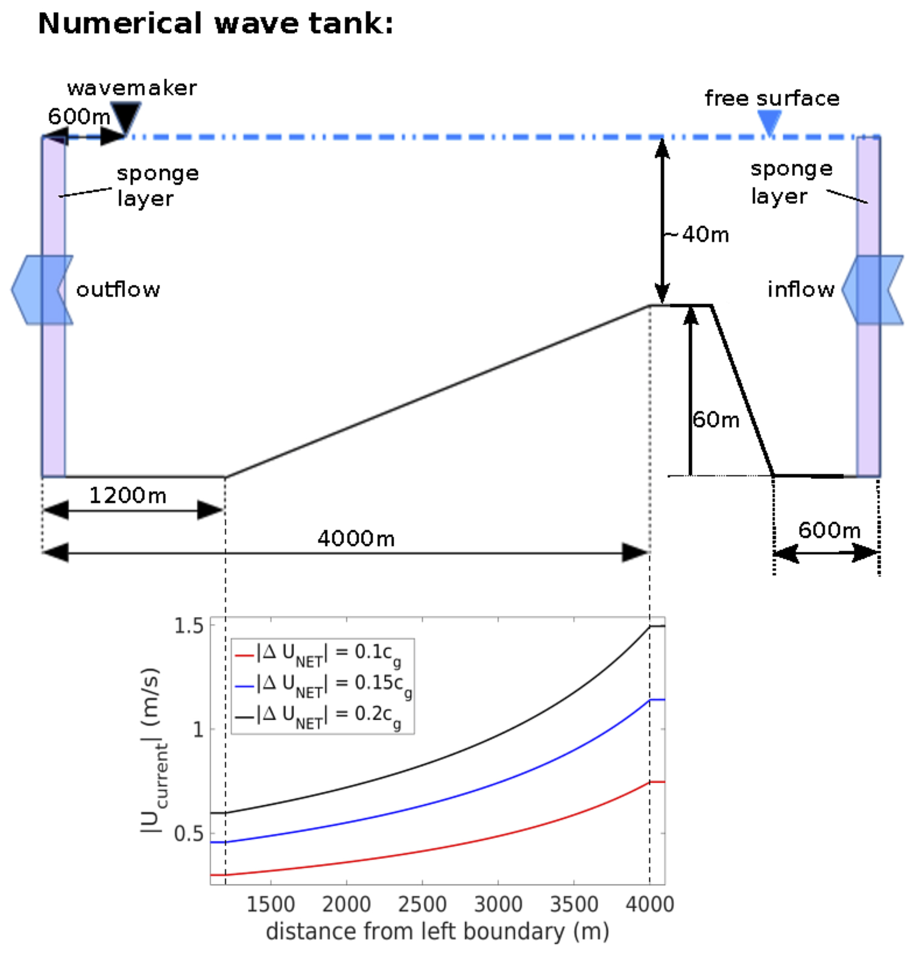
3.1. Model Setup

Our study focuses on wave evolution in deep water. In accordance with Airy wave theory, the minimum depth needed to be at least half the length of the longest wavelength. Computational limitations with respect to depth (for a given $\Delta z$) set limitations on the greatest wavelength that we could implement while maintaining a fixed minimum degree of vertical grid resolution (25 levels per 100 m depth). Similar limitations in the degree of horizontal mesh refinement that was computationally feasible set limits to the smallest possible wavelength in our simulations, as we wanted to simultaneously maintain $\Delta x=0.25$ m and keep a fixed minimum number of grid points per smallest wavelength. With these considerations taken into account, the wavemaker was configured to produce a spectrum with a minimum frequency equal to 0.14 Hz, a maximum frequency equal to 0.22 Hz, and a peak frequency approximately equal to 0.18 Hz, while a total of 110 different frequencies were produced within that range with random phase values. At this frequency range, the smallest wavelength was resolved horizontally by 130 grid points. The vertical grid resolution varied between $\Delta z=4$ m in the deepest part of the domain and $\Delta z\approx 1.6$ m at the shallowest part. The numerical wavemaker was adjusted so that the produced waves approximately fit the section of a JONSWAP spectrum in the frequency range implemented and with the same peak frequency. Individual wave steepness values and $H_s$ remained low in our simulations, while computed spectral peakedness values corresponded to a JONSWAP spectrum with shape factor $\gamma \approx 3.3$. Wave steepness values were measured as $k\frac{H}{2}$, where H is wave height and was computed as the surface elevation of the peak minus one-half the sum of the surface elevations of the two neighboring troughs. In our simulations, steepness values rarely exceeded 0.1.

With the chosen spectral parameters, the longest wavelength was approximately 80 m, necessitating a minimum depth of 40 m. Our numerical wave tank, seen in the top of Figure 1, had a length of approximately 5.1 km, with currents moving in the negative x-direction and waves traveling in the positive x-direction (starting near the left boundary). The wavemaker was situated 600 m from the left (outflow) boundary. Adverse current gradients were induced by gradually varying the depth of the domain, making it shallower in the positive x-direction. As the minimum allowable depth was fixed, the strength of the current gradient, as well as the total amount of current strength increase in the direction of wave propagation, $|\Delta U_{NET}|$, were controlled by adjusting the volumetric flow rate at the inlet/right boundary. We implemented gradients of three different profiles in our simulations (Figure 1, bottom), with $|\Delta U_{NET}|$ equal to 0.1$c_g$, 0.15$c_g$, and 0.2$c_g$. These fractions of group velocity, $c_g$, representing $|\Delta U_{NET}|$ are comparable to values used in experiments with wave tanks [20,21,22,23]. On the basis of the chosen spectral parameters and Equation (3), where current strength is scaled by the undisturbed speed of wave propagation ($\frac{1}{2}{c}_p$), the strongest current gradient that we tested, with $|\Delta U_{NET}|=0.2c_g$, corresponds to a current gradient in the ocean with $|\Delta U_{NET}|\approx 1.6$ m/s. Considering that the strongest currents in the ocean rarely exceed 2 m/s [34], the gradient strength values that we tested correspond well to actual oceanic conditions. As illustrated in the top of Figure 1, NHWAVE allows for the combination of wave-absorbing sponge layers (pink color), as well as a prescribed inflow volume flow rate at the right boundary. The sponge layer widths were set at 200 m, and, at that value, proved highly effective at completely absorbing incoming waves. The currents that we applied in our simulations transitioned from a minimum to a maximum strength over a distance spanning 2.8 km ($\approx 60{\lambda }_{peak}$), starting at $x_o$ = 1200 m and attaining maximum strength at $x=4000$ m. This marks a different approach from what has been followed so far numerically and experimentally, whereby current transitions occurred over shorter distances ($\approx 10{\lambda }_{peak}$), and where the researchers focused on wave characteristics before and after the gradients were traversed. Our approach, on the other hand, was to implement currents transitioning more slowly and allow traveling waves to absorb all of the energy made available to them by the current gradient while we monitored wave evolution in the process. The current velocity profiles in our simulations (Figure 1, bottom) were known to us, and we were able to derive accurate analytical formulas to characterize them by implementing polynomial fitting. While the domain depth varied linearly in our numerical wave tanks, the current velocity profiles did not, something explained by the nonlinearity of the flow equations. Computing an analytical formula for current strength allowed for the calculation of a theoretical wave-energy gain at every point spanned by the current gradient on the basis of a quasi-steady-state approximation by utilizing Equation (3), where $\Delta U(x)=U(x)-U(x_o)$.

We should note that we use the term wave-energy (or energy) to refer to power spectral density integrated over frequency, i.e., the total energy of the spectrum; although the latter is not energy and has different units, it is proportional to wave-energy. The wave frequency spectrum was derived by performing a discrete fast Fourier transform (DFFT) on the time series of the free surface, while Hann windowing, as well as time ensembling, were implemented in the computation sequence.

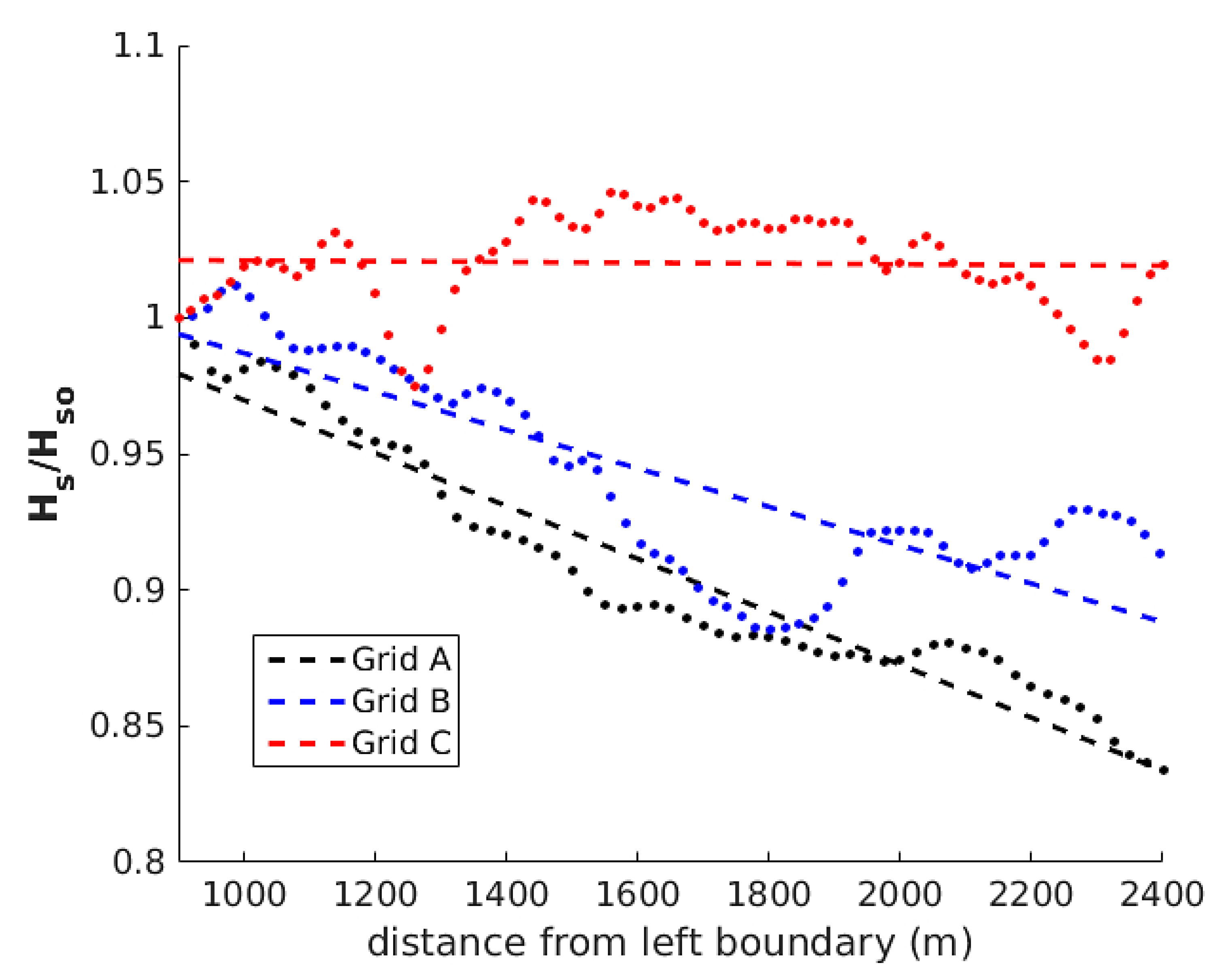
3.2. Grid Resolution and Convergence Testing

The scales that we desired to implement made some amount of numerical diffusion (also known as numerical dissipation) unavoidable, even with the implementation of second-order spatial and temporal accuracy. In numerically solving the Euler equations, the momentum fluxes are algebraic expressions of first-order difference formulas. While the HLL flux scheme is second-order accurate in space, the van Leer limiter that is used to compute velocity gradients causes the flux scheme to be dissipative [30], and the truncation error contains even-numbered velocity derivatives in the lowest order. Several of the dissipative terms in the truncation error increase in magnitude when a horizontal current is applied.

It was necessary to characterize our model in terms of such artifacts, especially since applying horizontal currents against the direction of wave propagation noticeably increased the rate of numerical dissipation, as we show in Appendix A. For that purpose, we conducted a grid-refinement study, where we used three grids of different resolution, as shown in

Table 1. Characteristics of grids used in the grid-refinement study.

Grid	$\Delta \mathit{x}$ (m)	$\Delta \mathit{z}$ (m)
A	0.25	4.0
B	0.22	2.0
C	0.20	1.33

.

Random waves of spectral characteristics, like those described in Section 3.1, were produced and propagated against a current of fixed strength, ≈$0.17c_g$, in deep water of constant depth equal to 100 m. We applied a current in our convergence study in order to produce conditions similar to those in the main simulations. We monitored the significant wave height and its gradual drop due to numerical dissipation as waves traversed the domain. The evolution of $H_s$ for the three grids is presented in Figure 2. The BFI was computed in all three cases and was found to be ≤0.5. The variability in computed $H_s$ values, which is more pronounced in the case of the two finer grids, was due to the shortness of simulation durations imposed on us by restrictions on computational resources.

With consideration to spectral stability analysis [30], it is expected that the amount of amplitude loss with every time iteration for a wave of some wavelength, $\lambda$, depends on the ratios $\frac{\Delta x}{\lambda }$, $\frac{\Delta z}{\lambda }$, as well as the CFL numbers, $\frac{{\alpha }_x\Delta t}{\Delta x}$ and $\frac{{\alpha }_z\Delta t}{\Delta z}$, where ${\alpha }_x$ and ${\alpha }_z$ are the x- and z-direction flow speeds. The time step, $\Delta t$, is adjusted in NHWAVE so that $CF{L}_{max}=0.5$ at every time step. Consistency would then require the drop in $H_s$ due to numerical dissipation to be reduced as the level of horizontal and vertical grid refinement is increased, which was actually observed in our grid refinement study, as shown in Figure 2.

We also assessed the degree of dispersion error associated with the phase speed of the peak frequency, defined as the ratio of numerical to theoretical wave celerities [30]. The results of that comparison are summarized in

Table 2. Dispersion error in grids of varying resolution.

Dispersion Error	Grid A	Grid B	Grid C
$c_{p,n}/c_p$	1.050	0.954	0.973

. As in the case of the results with respect to $H_s$ drop, the dispersion error decreased with increasing levels of grid refinement. Interestingly, while the low grid resolution case proved slightly dispersive, the pattern of refinement that we followed in our study caused the numerical phase speed to shift to below the theoretical value.

The consistency of the model is shown by our grid-refinement study, while stability is maintained in NHWAVE by implementing adaptive time-stepping. The solutions that NHWAVE provided in our simulations thus demonstrably converged toward the exact solutions to the Euler equations and were accurate to the degree that the level of grid refinement allowed. With the study, we also verified the numerical nature of the energy-dissipative effects that we were witnessing in our simulations, and which worsened in the presence of currents, as those subsided with increasing grid refinement.

The resolutions used in Grid B and Grid C were prohibitive with respect to computation time for running a large ensemble of simulations. For numerical efficiency, we used the resolution of Grid A in our main simulations, and we adopted a procedure that accounted explicitly for numerical energy dissipation. The procedure is described in detail in Appendix A and is essentially a way by which we calibrated our model so that errors due to wave-energy loss caused by numerical dissipation do not enter our final calculations for assessing the current gradient-induced wave-energy gain.

4. Results

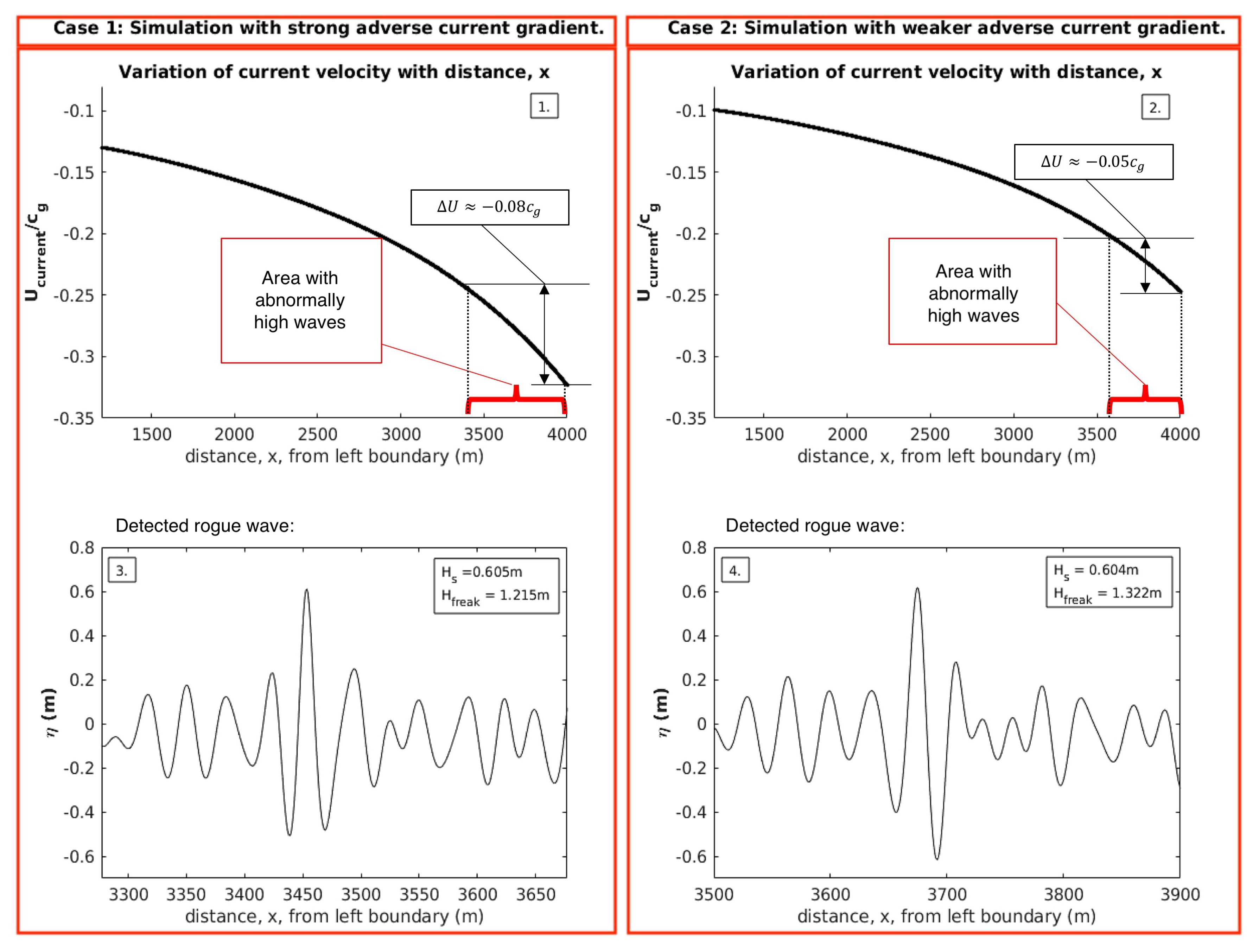
4.1. Qualitative Analysis: Observation of Rogue Waves and of Changes in Wave Characteristics Induced by Adverse Current Gradients

Of the three main simulations that were carried out, rogue waves were observed in the two with the stronger current gradients, which we refer to as Case 1 and Case 2. The current velocity profiles pertaining to those cases are shown in Figure 3 (subplots 1 and 2), where the ratio $\frac{U_{current}}{c_g}$ is plotted as a function of distance, x. The profiles are accurately described as fourth-order polynomials of x, with both current velocity, $U_{current}$, and current gradient, $\frac{\partial U_{current}}{\partial x}$, negative and decreasing monotonically with x, with the positive direction being that of wave propagation. Case 1 involved the strongest current gradient that we tested, with $\Delta U_{Net}\approx -0.2c_g$, while, for Case 2, $\Delta U_{Net}\approx -0.15c_g$. Both cases simulated 2000 s of wave propagation, and one rogue wave was detected in simulation Case 1, while several other waves came very close to fulfilling the rogue wave criterion ($H_{rogue}\ge 2H_s$). Several rogue waves were detected in Case 2, with the highest having $H_{rogue}=2.18H_s$ (shown in subplot 4).

Rogue waves and waves that were nearly as high were detected solely in the last stretch of the current gradient zone in both cases ($3400\mathrm{m}\le x\le 4000\mathrm{m}$—red brackets in subplots 1 and 2 of Figure 3). Figure 4 shows computed wave characteristics in an area containing that region. Shown in subplots 1 and 2 of that figure is the increase in $k_p$ with x induced by the Doppler shift. There was some uncertainty in determining the peak wavelength from time series data, which is reflected in the computed $k_p$ values, but, on average, $k_p$ varied in good agreement with theory, given by [19]:

$$k_p(x)=(g+2\pi f_{p}U(x)-\sqrt{g^2+8g\pi f_{p}U(x)})/(2U^2(x)).$$

(7)

where $U(x)$ is the current velocity at x, g is the acceleration of gravity, and $f_p$ is the peak frequency. It is seen that $k_p$ increases more rapidly with x for higher values of x, which is expected considering the aforementioned characteristics of the current gradient profiles.

Spectral peakedness values increased abruptly in the areas of the domain where unusually high waves were observed, as shown in subplots 3 and 4 of Figure 4. Spectral narrowness followed a trend similar to that of spectral energy in our simulations, i.e., there was competition between current gradient-induced energy gain versus energy loss due to numerical dissipation. More on numerical dissipation is explained in Appendix A. In both simulations, in the final 600 or so meters of the current gradient zone, there was a net energy increase with x, with current-induced energy gain exceeding numerically induced energy loss, with the trend being reflected in spectral peakedness values. Spectral peakedness was computed by two different methods, outlined in Rogers and Van Vledder [35]. Referring to the work by the authors, we computed the spectral narrowness parameters $Q_C$ and $Q_D$ (red and blue plots, respectively, in subplots 3 and 4 of Figure 4), with the former given by:

$$Q_C=max(E_{fn})/T_{m,-1,0},$$

(8)

where $E_{fn}=E(f)/\int E(f)df$, and where $T_{m,-1,0}=\int f^{-1}E(f)df/\int E(f)df$ is the mean spectral period ($E(f)$ is the spectral density at f). The parameter $Q_D$ was first introduced by Goda [36] and is computed as:

$$Q_D=2{(\int E(f)df)}^{-2}(\int f{E}^2(f)df).$$

(9)

We note that a definition for the BFI that is alternative to that given by Equation (1) appears in the literature [35] as:

$$BFI=\sqrt{2\pi }{k}_p\sqrt{E}{Q}_D.$$

(10)

In the Case 1 and Case 2 simulations, the increase in $k_p$, compounded with the net energy increase and the ‘jump’ seen in spectral peakedness in the last 600 m of the domain, all amounted the BFI increasing by more than 50% of its value up to that point. Subplots 5 and 6 of Figure 4 show how the computed kurtosis values varied with x in our simulations and indicate a small but noticeable departure from Gaussian statistics in the region of interest. We should note that it was not surprising to us that only one rogue wave was observed in Case 1, which involved the strongest current gradient, while several rogue waves were observed in Case 2; Case 1 involved a stronger current gradient, but, as was explained in Section 3.2 and is also explained in Appendix A, numerical dissipation energy loss was also more pronounced in Case 1. The end result is that Cases 1 and 2 featured comparable changes in energy gain-induced spectral narrowness and, ultimately, kurtosis, as shown in Figure 4.

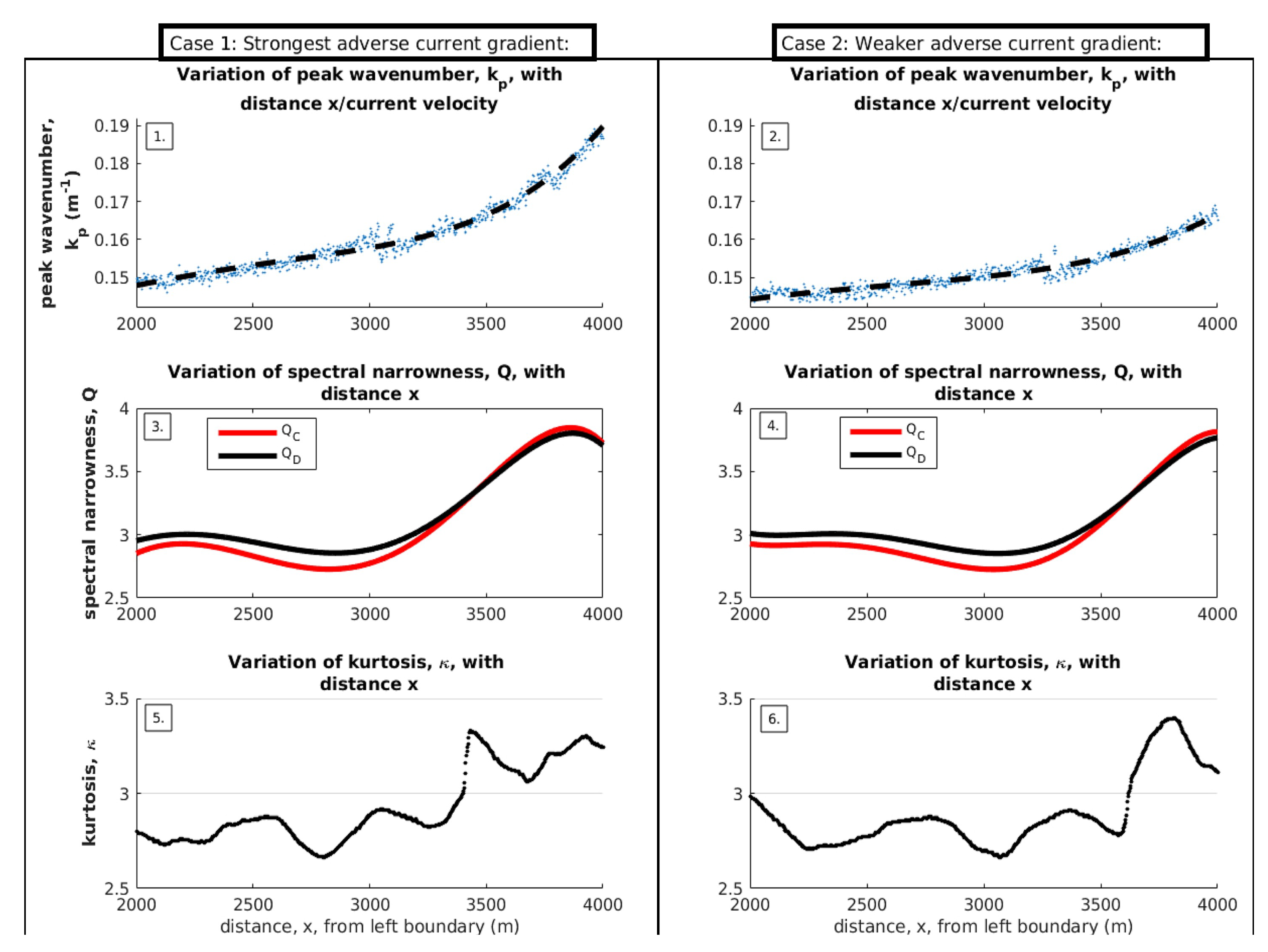
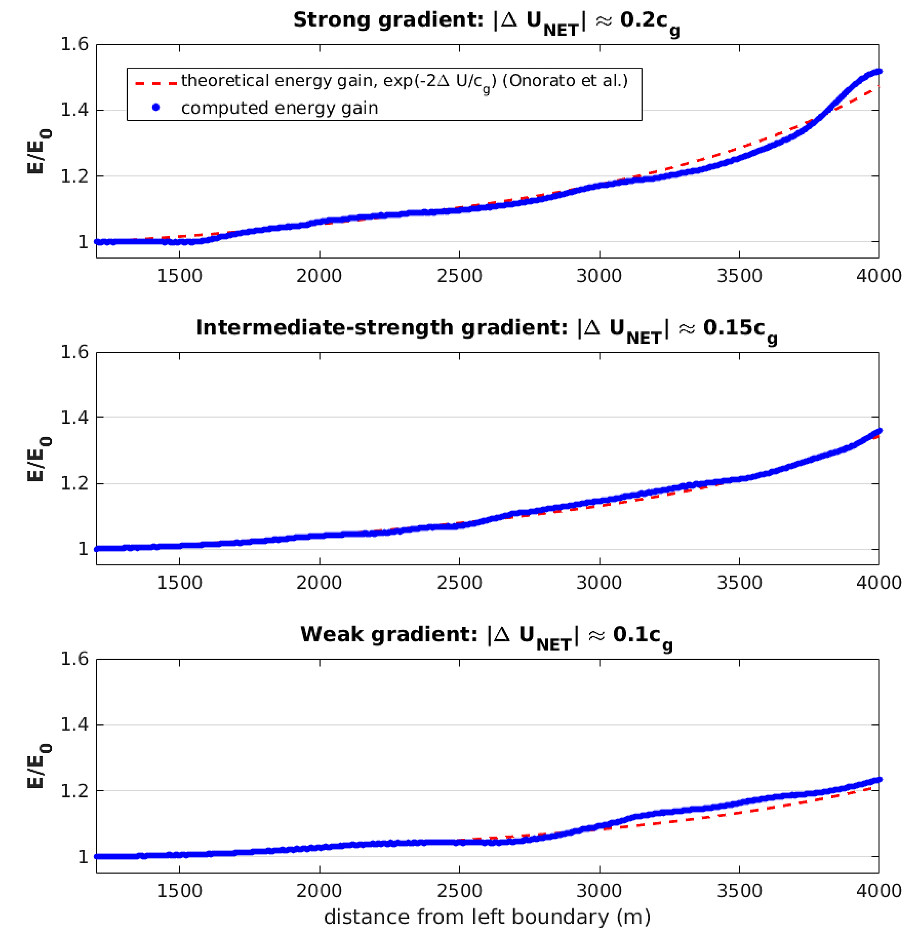
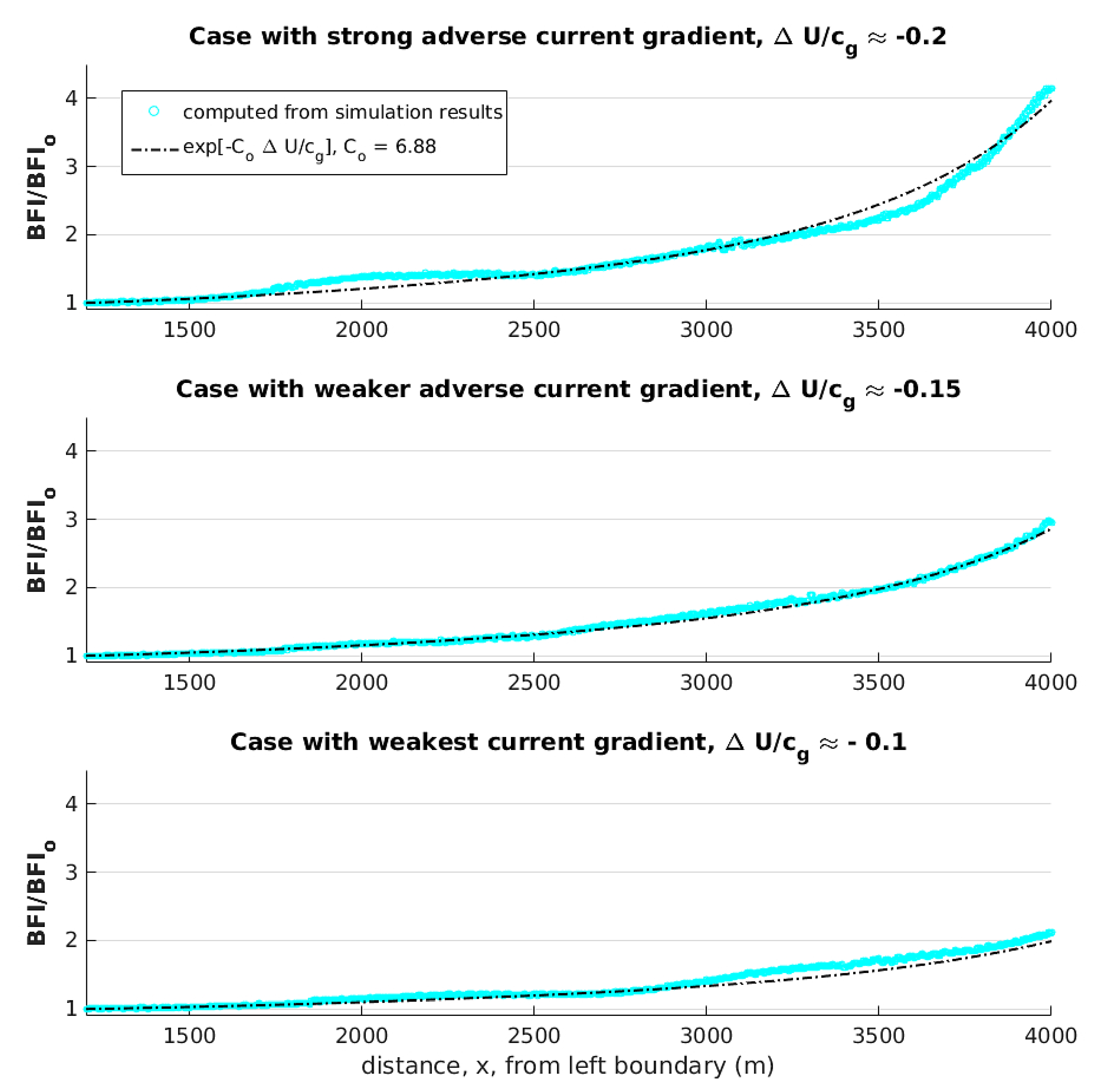
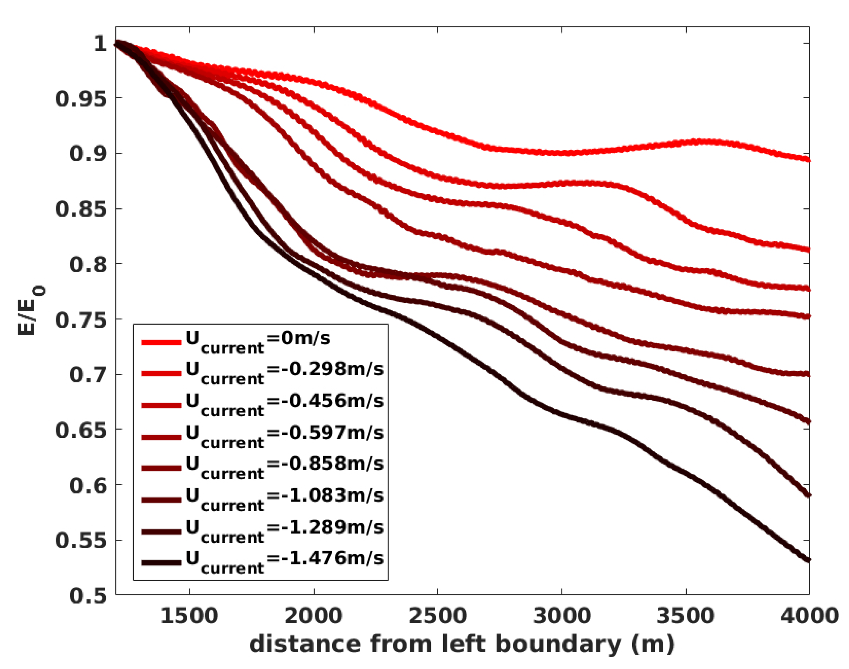
4.2. Quantitative Analysis: Estimating Current Gradient-Induced Energy Gain and BFI Increase

Current gradient-induced energy gain was estimated by analyzing time series data and by calibrating our model to account for numerical dissipation losses, as is explained in Appendix A. In Figure 5, we compare our computed estimates with theoretical values on the basis of studies of the NLS [18], as given by Equation (3). The RMS error is 0.0146, and the corrected model output is within 0.9% of theory.

In calculating the theoretical energy gain in Figure 5, as given by Equation (3), $c_g$ was estimated using the numerical peak phase velocity, $0.5c_{p,n}$.

On the basis of our computed estimate for current-induced energy gain, as produced by our calibrated model, and by utilizing the BFI definition given by Equation (10), we were able to compute an estimate for the current gradient-induced increase in the BFI. In doing so, we also derived ‘calibrated’ estimates of the increase in spectral narrowness which were devoid of the effects of numerical dissipation energy loss. The estimates for the BFI increase for the three different adverse current gradients in our main simulations are shown in Figure 6, where we fitted an exponential of the form

$$BFI=BF{I}_{o}exp(C_o\frac{-\Delta U}{c_g})$$

(11)

to computed values.

5. Discussion and Conclusions

The goal of our study is to quantify the effect of opposing current gradients on propagating waves in deep water in a manner that is most generally applicable and of use to seafaring entities around the world. We utilized CFD tools in order to solve the inviscid Euler equations of fluid motion and to simulate mild waves traveling against adverse current gradients. We first carried out grid-refinement studies that demonstrated convergence of our solution. We devised a procedure to calibrate our model to account for and correct errors incurred by numerical dissipation losses in our simulations.

In our main simulations, we monitored the evolution of wave characteristics and wave-energy as waves propagated against adverse current gradients. Our results showed a marked current gradient-induced wave-energy gain, which agreed well with theoretical estimates [18]. The energy gain was concentrated in a narrow bandwidth, which caused spectral narrowness values to rise. The energy gain together with the increase in spectral narrowness, as well as the Doppler shift-induced increase in peak wavenumber, had a pronounced effect on the BFI; the Benjamin–Feir instability was triggered, which caused the appearance of freak waves in two of our main simulations. From computed estimates of how wave characteristics change under the action of current gradients, we devised an empirical exponential formula which relates the current gradient-induced BFI increase to changes in current velocity.

We should note that, in our simulations, we detected and measured a counter-current generated by the traveling waves (a Stokes drift), with measurements agreeing with theory. We did not, however, adjust the current velocity profiles, $U(x)$, to account for it. The reason for this inaction lies in the manner in which the NLS, modified for a current (and Equation (3) that stems from it), was originally derived by Hjelmervik and Trulsen (2009) [12] and used further by others. The current velocity, U, and its derivative, $\frac{\partial U}{\partial x}$, as they appear in their work, refer to the prescribed current field, prior to being superposed to the wave-velocity field. The same terms later appear in Onorato et al. (2011) [18], and the term $\Delta U$ in Equation (3) stems from simply integrating $\frac{\partial U}{\partial x}$ over x. $\Delta U$ then refers to the initial, prescribed state of the current prior to being altered in any way by the presence of waves.

For reasons that were already explained, we restricted our wave-current simulations to two dimensions. Equation (11) can be modified to be applicable to directional wave spectra by adjusting $BF{I}_o$ for directionality following one of the many proposed approaches that exist in the literature [9,37,38]. In the scenario whereby peak-frequency waves travel at some angle, $\theta$, with respect to the current flow velocity, we adjusted Equation (11) as follows:

$$BFI=BF{I}_{Do}exp(C_o\frac{-\Delta Ucos(\pi -\theta )}{c_g}).$$

(12)

In Equation (12), $BF{I}_{Do}$ is the BFI modified for spectral directionality, while only the component of the current velocity that is diametrically opposed to wave propagation enters the exponent [23].

The empirical relation (Equation (11)) that we propose, which relates the BFI increase to current velocity change, has no direct applicable theoretical counterpart. With respect to the method by which the relation was derived, computed estimates of energy gain and of current-induced shift in $k_p$ were both in good agreement with theory. Computed estimates of the increase in spectral peakedness were derived after calibrating our model for numerical dissipation energy losses, and those estimates involve some degree of uncertainty. The coefficient $C_o$ in the formula is to be further calibrated and validated with additional numerical simulations, experimental results, and field observations as data become available.

References

- Benjamin, T.B.; Feir, J.E. The disintegration of wave trains on deep water: Part 1. Theory. J. Fluid Mech. 1967, 27, 417–430. [Google Scholar] [CrossRef]
- Kharif, C.; Pelinovsky, E. Physical mechanisms of the rogue wave phenomenon. Eur. J. Mech. B Fluids 2003, 22, 603–634. [Google Scholar] [CrossRef] [Green Version]
- Manzetti, S. Mathematical modeling of rogue waves: A survey of recent and emerging mathematical methods and solutions. Axioms 2018, 7, 42. [Google Scholar] [CrossRef]
- Tulin, M.; Waseda, T. Laboratory observations of wave group evolution, including breaking effects. J. Fluid Mech. 1999, 378, 197–232. [Google Scholar] [CrossRef]
- Waseda, T.; Tulin, M. Experimental study of the stability of deep-water wave trains including wind effects. J. Fluid Mech. 1999, 401, 55–84. [Google Scholar] [CrossRef]
- Chabchoub, A.; Hoffman, N.P.; Akhmediev, N. Rogue wave observation in a water wave tank. Phys. Rev. Lett. 2011, 106, 204502. [Google Scholar] [CrossRef]
- Babanin, A.V.; Rogers, W.E. Generation and limiters of rogue waves. Int. J. Ocean Clim. Syst. 2014, 5, 39–49. [Google Scholar] [CrossRef]
- Babanin, A.V.; Waseda, T.; Shugan, I.; Hwung, H.-H. Modulational instability in directional wave fields, and extreme wave events. In Proceedings of the ASME 2011 30th International Conference on Ocean, Offshore and Arctic Engineering, Rotterdam, The Netherlands, 19–24 June 2011. [Google Scholar]
- Babanin, A.V.; Waseda, T.; Kinoshita, T.; Toffoli, A. Wave breaking in directional wave fields. J. Phys. Oceanogr. 2011, 41, 145–156. [Google Scholar] [CrossRef]
- Janssen, P.A.E.M. Nonlinear four-wave interactions and freak waves. J. Phys. Oceanogr. 2003, 33, 863–884. [Google Scholar] [CrossRef]
- Ankiewicz, A.; Crespo, J.M.S.; Chowdhury, M.A.; Akhmediev, N. Rogue waves in optical fibers in presence of third-order dispersion, self-steepening, and self-frequency shift. J. Opt. Soc. Am. B 2013, 30, 87–94. [Google Scholar] [CrossRef]
- Hjelmervik, K.B.; Trulsen, K. Freak wave statistics on collinear currents. J. Fluid Mech. 2009, 637, 267–284. [Google Scholar] [CrossRef]
- Adcock, T.A.A.; Taylor, P.H. The physics of anomalous (‘rogue’) ocean waves. Rep. Prog. Phys. 2014, 77, 105901. [Google Scholar] [CrossRef]
- Zakharov, V. Stability of periodic waves of finite amplitude on the surface of a deep fluid. J. Appl. Mech. Tech. Phys. 1968, 9, 190–194. [Google Scholar] [CrossRef]
- Onorato, M.; Osborne, A.R.; Serio, M.; Bertone, S. Freak waves in random oceanic sea states. Phys. Rev. Lett. 2001, 86, 5831. [Google Scholar] [CrossRef]
- Mori, M.; Janssen, P.A.E.M. On kurtosis and occurrence probability of freak waves. J. Phys. Oceanogr. 2006, 36, 1471–1483. [Google Scholar] [CrossRef]
- Lavrenov, I.V. The wave energy concentration at the Agulhas current off South Africa. Nat. Hazards 1998, 17, 117–127. [Google Scholar] [CrossRef]
- Onorato, M.; Proment, D.; Toffoli, A. Triggering rogue waves in opposing currents. Phys. Rev. Lett. 2011, 107, 184502. [Google Scholar] [CrossRef]
- Ruban, V.P. On the nonlinear schrödinger equation for waves on a nonuniform current. JETP Lett. 2012, 95, 486–491. [Google Scholar] [CrossRef]
- Ma, Y.; Ma, X.; Perlin, M.; Dong, G. Extreme waves generated by modulational instability on adverse currents. Phys. Fluids 2013, 25, 114109. [Google Scholar] [CrossRef]
- Toffoli, A.; Waseda, T.; Houtani, H.; Kinoshita, T.; Collins, K.; Proment, D.; Onorato, M. Excitation of rogue waves in a variable medium: An experimental study on the interaction of water waves and currents. Phys. Rev. E 2013, 87, 051201. [Google Scholar] [CrossRef] [Green Version]
- Toffoli, A.; Waseda, T.; Houtani, H.; Cavaleri, L.; Greaves, D.; Onorato, M. Rogue waves in opposing currents: An experimental study on the deterministic and stochastic wave trains. J. Fluid Mech. 2015, 769, 277–297. [Google Scholar] [CrossRef]
- Toffoli, A.; Cavaleri, L.; Babanin, A.V.; Benoit, M.; Bitner-Gregersen, E.M.; Monbaliu, J.; Onorato, M.; Osborne, A.R.; Stansberg, C.T. Occurence of extreme waves in three-dimensional mechanically generated wave fields propagating over an oblique current. Nat. Hazards Earth Syst. Sci. NHESS 2011, 11, 895–903. [Google Scholar] [CrossRef]
- Shrira, V.I.; Slunyaev, A.V. Nonlinear dynamics of trapped waves on jet currents and rogue waves. Phys. Rev. E 2014, 89, 041002. [Google Scholar] [CrossRef]
- Ablowitz, M.J.; Baldwin, D.E. Nonlinear shallow ocean-wave soliton interactions on flat beaches. Phys. Rev. E 2012, 86, 036305. [Google Scholar] [CrossRef] [PubMed]
- Gerber, M. The Benjamin-Feir instability of a deep-water Stokes wavepacket in the presence of a non-uniform medium. J. Fluid Mech. 1987, 176, 311–332. [Google Scholar] [CrossRef]
- Ardhuin, F.; Gille, S.T.; Menemenlis, D.; Rocha, C.B.; Rascle, N.; Chapron, B.; Gula, J.; Molemaker, J. Small-scale open ocean currents have large effects on wind wave heights. J. Geophys. Res. Oceans 2017, 122, 4500–4517. [Google Scholar] [CrossRef] [Green Version]
- Romero, L.; Lenain, L.; Melville, W.K. Observations of surface wave-current interaction. J. Phys. Oceanogr. 2017, 47, 615–632. [Google Scholar] [CrossRef]
- Ma, G.; Shi, F.; Kirby, J.T. Shock-capturing non-hydrostatic model for fully dispersive surface wave processes. Ocean Model. 2012, 43–44, 22–35. [Google Scholar] [CrossRef]
- Hirsch, C. Numerical Computation of internal & external flows. In The Fundamentals of Computational Fluid Dynamics, 2nd ed.; Butterworth-Heinemann: Burlington, MA, USA, 2007; ISBN 978-0-7506-6594-0. [Google Scholar]
- Harten, A.; Lax, P.D.; Van Leer, B. On upstream differencing and Godunov-type schmes for hyperbolic conservation laws. SIAM Rev. 1983, 25, 35–61. [Google Scholar] [CrossRef]
- Derakhti, M.; Kirby, J.T.; Shi, M.G. NHWAVE: Model Revisions and Tests on Wave Breaking in Shallow and Deep Water; Research Report No. CACR-15-8; University of Delaware: Newark, DE, USA, 2015. [Google Scholar]
- Ardhuin, F.; Chapron, B.; Collard, F. Observation of swell dissipation across oceans. J. Geophys. Res. Oceans 2017, 36, 1–5. [Google Scholar] [CrossRef]
- Gross, M.G. Oceanography, 6th ed.; Merrill: Columbus, OH, USA, 1990. [Google Scholar]
- Rogers, W.E.; Van Vledder, G.P. Frequency width in predictions of windsea spectra and the role of the nonlinear solver. Ocean Model. 2013, 70, 52–61. [Google Scholar] [CrossRef]
- Goda, Y. Numerical experiments on wave statistics with spectral simulation. Rep. Port Harb. Res. Inst. 1970, 9, 57. [Google Scholar]
- Mori, N.; Onorato, M.; Janssen, P.A.E.M. On the estimation of the kurtosis in directional sea states for freak wave forecasting. J. Phys. Oceanogr. 2011, 41, 1484–1497. [Google Scholar] [CrossRef]
- Ribal, A.; Babanin, A.V.; Young, I.; Toffoli, A. Recurrent solutions of the Alber equation initialized by Joint North Sea Project spectra. J. Fluid Mech. 2013, 719, 314–344. [Google Scholar] [CrossRef]
- Rap, A.; Ghosh, S.; Smith, H.M. Shepard and Hardy Multiquadric Interpolation Methods for Multicomponent Aerosol-Cloud Parametrization. J. Atmos. Sci. 2009, 66, 105–115. [Google Scholar] [CrossRef]