Article

Energetic Potential Assessment of Wind-Driven Waves on the South-Southeastern Brazilian Shelf

by
Phelype Haron Oleinik
1,*,
Eduardo de Paula Kirinus
1,
Cristiano Fragassa
2,
Wiliam Correa Marques
3 and
Juliana Costi
3
1
Engineering School, Federal University of Rio Grande, Campus Carreiros, Itália Avenue Km 8, Rio Grande 96230–000, Brazil
2
Department of Industrial Engineering, University of Bologna, Viale Risorgimento 2, 40136 Bologna, Italy
3
Institute of Mathematics, Statistics and Physics, Federal University of Rio Grande, Campus Carreiros, Itália Avenue Km 8, Rio Grande 96230–000, Brazil
*
Author to whom correspondence should be addressed.
J. Mar. Sci. Eng. 2019, 7(2), 25; https://doi.org/10.3390/jmse7020025
Submission received: 30 November 2018 / Revised: 14 January 2019 / Accepted: 21 January 2019 / Published: 23 January 2019
(This article belongs to the Special Issue Advances in Ocean Wave Energy Conversion)

Abstract

:
Global electric energy demand is constantly growing, consequently leading towards the usage of renewable energy sources reducing pollution and increasing sustainability. The ocean is a poorly explored renewable energy source; thus, to evaluate the Brazilian wave energy budget, this study investigated the mean behaviour of the wave power rate on the south-southeastern Brazilian Shelf as well as analysed the temporal variability of the wave power rate at the most energetic locations near the coast. Three locations were examined, namely Laguna, Ilhabela and Farol Island, based on the criteria of high means and small standard deviations. The mean wave power rate was approximately 9.08 kW / m on Laguna, 10.01 kW / m on Ilhabela and 15.93 kW / m on Farol Island. The standard deviation identified in the three locations reached values of 6.47 kW / m on Laguna, 7.59 kW / m on Ilhabela and 13.51 kW / m on Farol Island. Temporal variability analysis was conducted through wavelet analysis. The results show a dominant yearly cycle with a background presence of synoptic cycles, with little deviation between the locations. The El Niño southern oscillation plays a minor role on the energy spectrum of Laguna and does not have a significant influence on Ilhabela and Farol Island.

1. Introduction

Electrical energy has become essential for humanity and the demand of this resource grows rapidly. This fact has promoted research in this field and concerns about the environment. Several studies have focused on clean and renewable energy sources. Wave energy is one of the most environmentally friendly sources of energy because it is clean, inexhaustible and has no major impact on local hydrodynamics [1].
The first recorded attempt to use wave energy for human needs dates to the thirteenth century, but the efforts to convert it to electrical energy began in 1910, with a device similar to an Oscillating Water Column [2]. Driven by the oil crisis, both Europeans and Americans started studies and developments in wave energy technologies, but the funding of these studies declined after the decrease in oil prices a decade later. However, today, with the menace of oil shortage, wave energy is regaining its value in modern society [2].
Several studies have already been performed in the field of wave energy, from the development and enhancement of different conversion devices [3,4,5,6], to the theoretical assessment of wave energy availability, either by modelling [7,8,9] or by field data analysis [10,11,12].
To obtain an efficient farm to generate electricity from ocean waves, a thorough study has to be performed on different aspects of the implementation. In the global scope, this subject has already been widely studied by several authors. One of the first estimates was made by Isaacs and Seymour [13] who, based on the energy emitted by the Sun, guessed that the portion that corresponds to the waves is around 2.5 TW . More recently, Krogstad and Barstow [14] presented a map of the wave energy estimate around the world based on two years of data from Topex/Poseidon altimetry data. This result provided an early notion of the distribution of wave energy around the globe.
Later, with the increasing development of the wave models, wave energy resource studies became easier. Arinaga and Cheung [15] created an atlas of wave energy with detailed information on its temporal and spatial distribution. Their results, based on a 10-year dataset, present an interleaved winter–summer cycle between the northern and southern hemispheres, with higher energy in the winter. Reguero et al. [16] analysed a 60-year dataset and correlated the temporal variations of wave energy with the main climate anomaly indexes.
Gunn and Stock-Williams [17] used a directional approach for calculating the wave energy availability around the globe. Their study showed an even division of the wave energy budget for both hemispheres, with around 1 TW for each. On the other hand, a great disparity is noticed when comparing the energy availability between the continents, with 20% of it reaching the North American coastline. Another relevant conclusion by Gunn and Stock-Williams [17] is that, except for North America and Asia, all of the continents have wave energy sufficient to make up for their consumption.
The present study focused on the theoretical wave energy availability along the south-southeastern Brazilian Shelf (SSBS). Brazil is among the countries with the longest coastlines in the world, approximately 7500 km long, in which the southernmost 2777 km of coastline were approached in this work.
Neill and Hashemi [18] made a variability assessment of the waves around the British Isles that complements Arinaga and Cheung’s [15] study. These authors showed that, even though this location has an extremely high mean wave energy potential, the variability in this location is also elevated.
Several other studies on wave climate, focusing on their energetic potential, have been conducted over the last years in different parts of the world, e.g., by Stopa et al. [19] in Hawaii; Iglesias and Carballo [20] in El Hierro, part of the Canary Islands; Liang et al. [21] in east China; Hiles et al. [22] and Robertson et al. [23], both on the West Coast of Canada, which is more energetic than the East Coast; Hemer and Griffin [24] in south Australia; and Behrens et al. [25] on the entire Australian coast.
Wave power studies are extremely scarce on the Brazilian coast. Pianca et al. [26] assessed WaveWatch III data to evaluate the Brazilian wave climate. These authors classified the climate in terms of height, period and direction. They conducted the analysis for four seasons of the year and took measurements on six representative points of the Brazilian coast.
Parise and Farina [27] conducted a one-year simulation of the waves on the south Atlantic Ocean and collected data on the local wave climate. Losada et al. [28] conducted a 58-year-long analysis of the sea level properties of Latin America and quantified factors such as mean sea level rising trends, tidal variation, storm surges and the contribution of the El Niño southern oscillation.
The wave climate in Brazil was studied by Guimarães et al. [29,30] and Cuchiara et al. [31] with usage of the third generation model SWAN (Simulating Waves Nearshore) to simulate extreme events on the coast of the Rio Grande do Sul state. Parente et al. [32] approached dynamic patterns relating wave conditions to weather seasonality in the study region.
In terms of wave study along the Brazilian shelf, there is a visible dominance of studies on the waves of the Rio de Janeiro State due to its historical and economical importance. On the other hand, some studies on the Rio Grande do Sul State appear due to the importance of Rio Grande Harbour. Considering these factors, this study aimed to evaluate the wave climate on the south-southeastern Brazilian Shelf (Figure 1) to identify the energetic power of wind-driven waves and to provide information on variability and integrated values.
The following sections are organized as follows. Section 2 briefly describes the numerical model used in this work, the boundary conditions and the validation procedure. Section 3 is subdivided into three parts: a general analysis of the mean behaviour of the waves on the SSBS, a local mean analysis of the wave power at the most energetic point of the SSBS and the wavelet analysis to identify the temporal variability of these patterns at selected points. Section 4 contains the conclusions and final considerations of this study.

2. Materials and Methods

This study was based on the application of the third generation sea state model Tomawac to simulate wave conditions over the SSBS over a period of 18 years, between 1997 and 2014, using boundary conditions from WaveWatch III and wind data from NOAA’s Reanalysis 1. The data used were the integrated parameters Significant Wave Height (Hs), Mean Period (Tm) and Mean Direction (Dm) on the oceanic boundaries and the wind velocity on the free surface.

2.1. Numerical Model

The model Tomawac (Telemac-Based Operational Model Addressing Wave Action Computation) was used to conduct the numerical simulations. This model is a part of the modelling system Open Telemac-Mascaret1. Tomawac is a third generation model based on wave action density conservation (Equation (1)) [34,35,36]:
N t + x ˙ N x + y ˙ N y + k ˙ x N k x + k ˙ y N k y = Q k x , k y , x , y , t
where N represents the directional spectrum of wave action density, x and y are the coordinate system, k x and k y are the components on x and y of the wave number vector, t is the time, and the dot above a symbol denotes its time derivative. Equation (1) represents that, in a general situation of waves propagating in a non-homogeneous and unsteady environment, the wave action density is preserved within the source and sink terms, defined by Q.
Tomawac calculates wind-driven waves taking into account most of the main physical processes involved, such as shoaling, whitecapping, bottom friction-induced dissipation, nonlinear interactions between waves and depth-induced refraction, and all these effects were taken into account in the simulation. Tomawac, however, does not take diffraction and reflection into account [36].
To solve Equation (1), Tomawac splits the directional spectrum (N) into a finite number of wave frequencies ( f i ) and directions ( θ i ) and solves Equation (1) for each component ( f i , θ i ). The directional spectrum of wave energy, denoted by E ( f , θ ) , can be associated with the directional spectrum of wave action through Equation (2):
E ( f , θ ) = N ( f , θ ) . ρ g σ
where ρ is the specific mass of water, g is the gravity acceleration and σ is the angular frequency of the waves given by σ = 2 π f . The integration of E ( f , θ ) along the discretized frequencies and directions yields the energy per unit area of the random multi-directional waves (Equation (3)):
f f + d f θ θ + d θ 1 2 ρ g a m 2 = E ( f , θ ) d f d θ

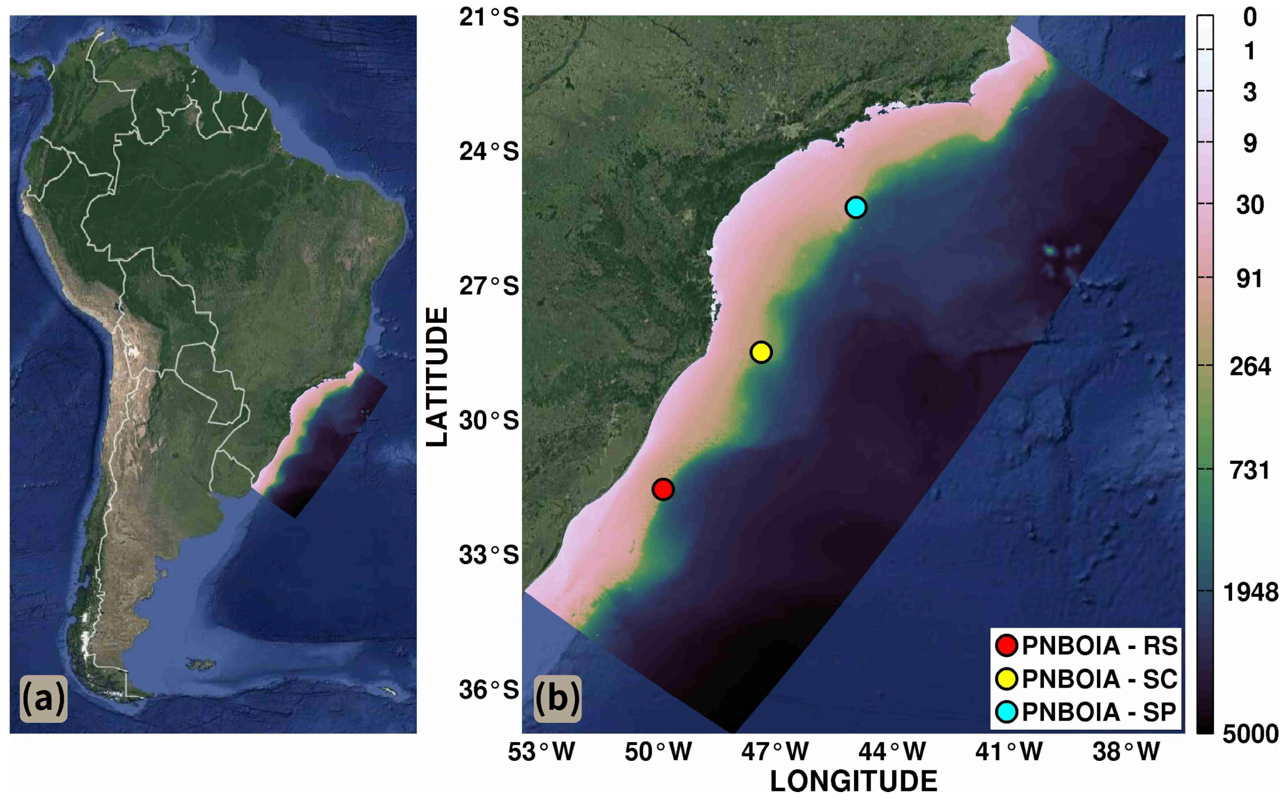
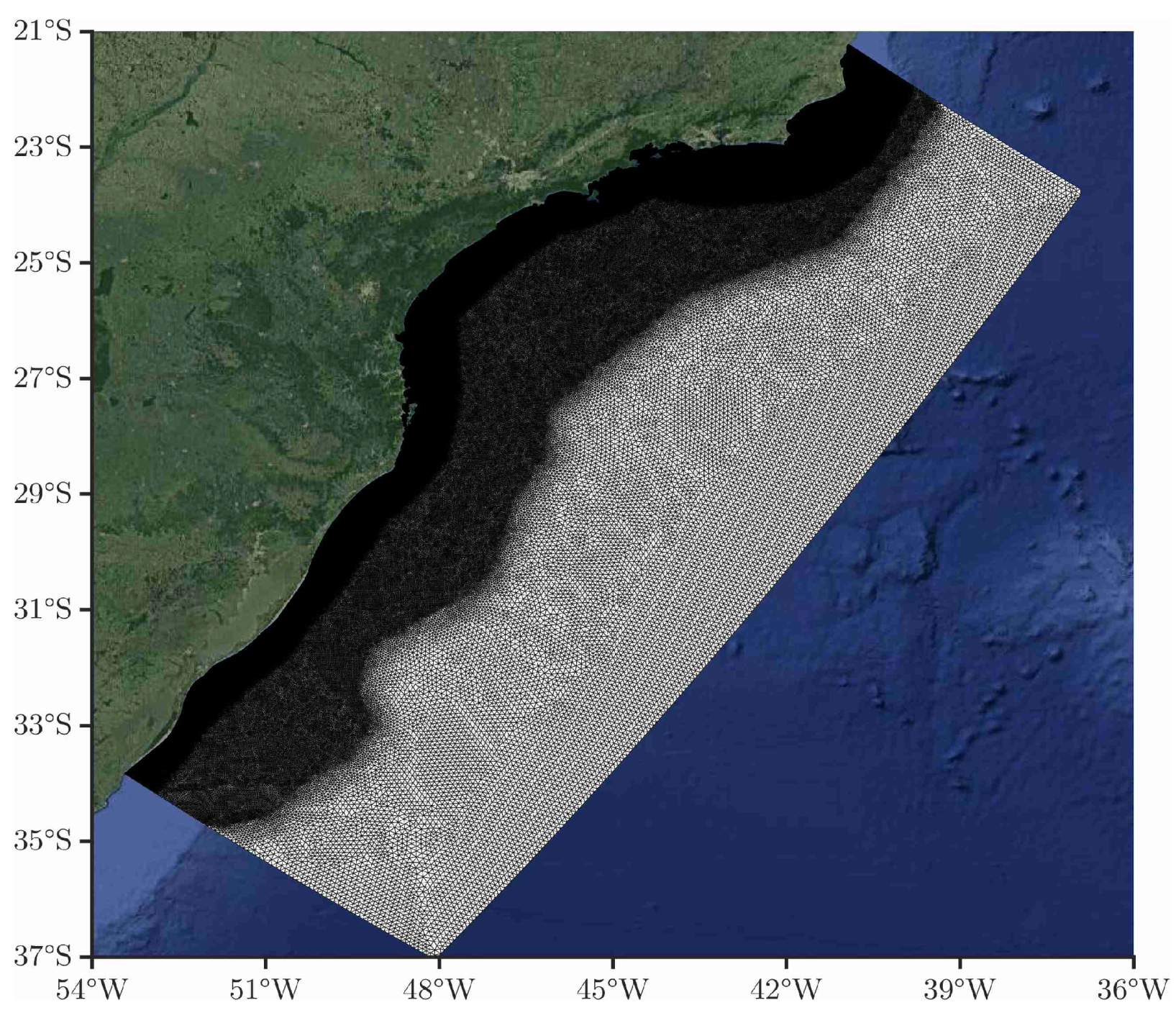
2.2. Boundary Conditions and Computational Grid
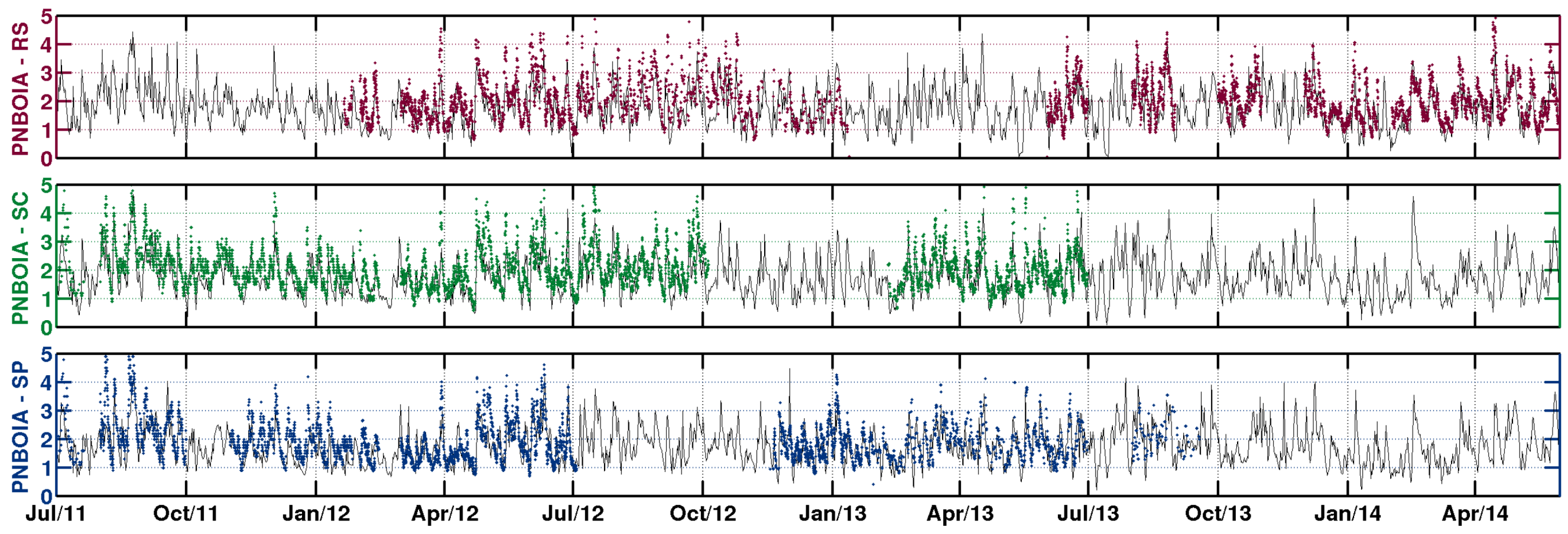
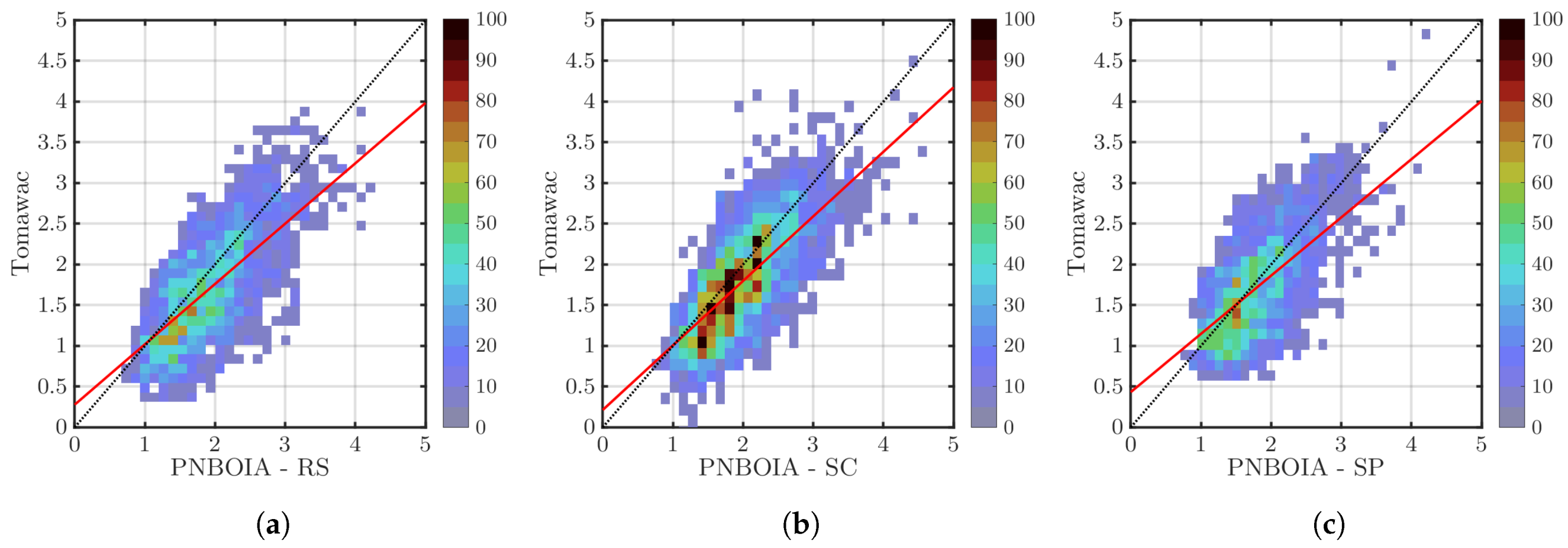
To perform the numerical simulations, data from NOAA’s (National Oceanic and Atmospheric Administration) wave forecasting model WaveWatch III2 [37,38,39] and from the NCEP/NCAR Reanalysis 13 [40] were used to represent the liquid and superficial boundaries of the model, respectively.
The model started from the rest and the surface boundary was set to winds from the NCEP/NCAR Reanalysis 1, with a temporal resolution of 6 h and a spatial resolution of 1.875° (T62 Gaussian Grid). These data were bilinearly interpolated to the numerical domain.
The oceanic boundaries were set by the imposition of the integrated parameters Hs, Tp (peak period) and Dm. The data were generated by WaveWatch III and have a spatial resolution of 30 arc minutes and a temporal resolution of 3 h. Bathymetric data were acquired from the Brazilian Navy Admiral Charts and from the GEBCO (General Bathymetric Chart of the Oceans) database.
The validation and the case study simulations used the same data sources. The validation simulation lasted four years, from 2011 to 2014, the period when data from PNBOIA (Programa Nacional de Boias) were available. The simulation for the case study lasted 18 years from 1997 to 2014.
The computational grid used in the simulations extents from the south of Rio Grande do Sul, in the border between Brazil and Uruguay, to the north of the state of Espírito Santo. The mesh also extents 650 km towards the ocean (Figure 1).
Figure 2 shows mesh used in the simulations. The mesh contains 405,833 triangular elements, totalling 205,617 nodes. The mesh has varying levels of refinement, from 8000 m between nodes in the oceanic region, 2500 m on the deep continental shelf, to 1000 m in regions shallower than 100 m . In regions of interest, the nodes are 300 m apart, approximately.
With this configuration, using Tomawac version v7p2r2 in scalar mode, the case study simulation took approximately four weeks to run on a Intel ® Core i7-4960X CPU @ 3.60 GHz × 12, using around 8 GiB of RAM. The results of the case study simulation were saved in a 75.7 G file.

2.3. Validation

The validation of the model was accomplished by comparing the time series of Hs and Tp from the Tomawac model with the time series measured by the wave buoys. The data used to validate the numerical model were obtained from PNBOIA on the coast of Rio Grande do Sul (31°34′ S 49°53′ W, 200 m depth), Santa Catarina (28°30′ S 47°22′ W, 200 m depth) and São Paulo (25°17′ S 44°56′ W, 200 m depth) (Figure 1). The datasets used had: 7749 data points at the buoy of Rio Grande do Sul, 8836 at the buoy of Santa Catarina, and 6988 data points at São Paulo.
The PNBOIA is an ongoing project for gathering and providing oceanographic and meteorological data along the Brazilian coast and the adjacent Atlantic Ocean. This project aims to contribute to the characterization of the Brazilian marine environment as well as to attend to the necessities of navigation security, oceanic meteorological forecasting and human life protection. The project, which counts with the assistance of several governmental institutions, has more than 300 buoys in its database providing information about oceanic circulation, water properties and waves and the associated atmospheric conditions.
The time series provide a visual representation of the comparison between Tomawac and the buoys. This comparison can be quantified for better understanding, using well known [41,42,43,44,45] error metrics in this field of study. The equations to compute these metrics are presented in Table 1. In the equations, T i are the data modeled by Tomawac, B i the data measured by the buoys and n the number of data entries in a time series. To complement the results, some statistics about the data from both Tomawac and the buoys are presented in Table 2 with the error metrics.
The comparison of the time series is shown in Figure 3, where their period range from 1 July 2011 to 31 April 2014. The time series shows that there is a close agreement between the model and the measured Hs.
To quantify the quality of the numerical results, some statistical parameters were calculated during periods in which there were data collected from the model and measurements (Table 2). Average values show that the model results approach the measured data. Nevertheless, on average, numerical results tend to underestimate empirical data.
These mean values are considerably robust for a wave prediction model. In their wave resource study, Edwards et al. [46] matched ECMWF’s (European Centre for Medium-Range Weather Forecasts) Cy331 WAve Model (WAM) with a Datawell Waverider Buoy and obtained a mean difference of 0.17 m . Studying wave energy power, Santos [47] found mean differences of approximately 0.30 m both in the calibration and in the validation of the numerical model. Melo et al. [43] found differences of approximately 0.22 m while assessing the results of the WaveWatch III model. Similar pattern of comparison was found by Iuppa et al. [48] validating the performance of SWAM model against satellite data.
Another statistical parameter calculated is the Root Mean Square Error (RMSE). This parameter is used because it makes larger errors more important than minor errors in calculating final results. RMSE is a widely used statistical parameter [43,46,47] for this type of analysis because, as the models are never perfectly adequate, RMSE neglects small differences in a time series that are not considered significant errors. The RMSE of the Hs is an average 0.5 m , a slightly lower value than values calculated in other calibration and validation studies [42,43,46,47].
The mean Tp is underestimated by Tomawac with a difference of approximately 0.9 s . The results obtained by Lalbeharry [42], Melo [43], and Santos [47] show approximately the same mean difference. Although the calibration and validation of wave models is primarily based on the Hs parameter, due to the amount of errors in the Tp data measured by the buoy, some filters can be applied to clean the data, and this often results in a robust correlation between the model and measured Tp. The RMSE is approximately 2.0 s , which is comparable with aforementioned studies.
The correlation coefficient for Hs is between 0.88 and 0.91, the lowest value being found near the coast, indicating a less strong correlation at this region. For Tp, the correlation coefficient is slightly higher than for Hs (between 0.89 and 0.93) indicating the same level of correlation for both parameters.
To conduct the last verification of the model validation, the Scatter Index (SI) was calculated for the two parameters. The advantage of SI is that being dimensionless, contrary to the RMSE, it can be compared for the same or different variable and, among different magnitudes of data, allowing the comparison between ocean and coastal zones. Based on the SI values, Hs calculated in deep regions is slightly more precise than Hs calculated near the near shore. Additionally, the model output for Tp approximates the measured data better than values of Hs.
Finally, to visualise the correlation between the measured data and Tomawac’s results, scatter plots were created correlating both datasets. Figure 4 shows the scatter plots of the three validation datasets used. The scatter plots were made using discrete bins to avoid the cluttering caused by the large amount of data points.
The plots in Figure 4 emphasize the conclusions drawn above. The data are distributed along the 45° line with some scattering, which lowers the correlation coefficient. The solid diagonal lines in each scatter plot shows the linear regression of the dataset comparison. The linear regression enhances the slight underestimation of the wave heights by Tomawac; Cavaleri [49] pointed out a few sources of underestimation from wave models as being related to whitecapping processes and non-linear interactions. Nevertheless, the correlation between measured and modelled wave heights is satisfactory, although the issue of the underestimation could, in a future study, be addressed with a different calibration.

3. Results and Discussion

To investigate the energetic power of wind-driven waves along the SSBS, a long-term simulation was conducted over 18 years from January 1997 to December 2014. The results were investigated using mean values to identify the most energetic points near the coastal region. Spatial and temporal variability of wave power and wind intensity were investigated using wavelet analysis that was conducted following the methods of Torrence and Compo [50] and the bias correction proposed by Liu [51].

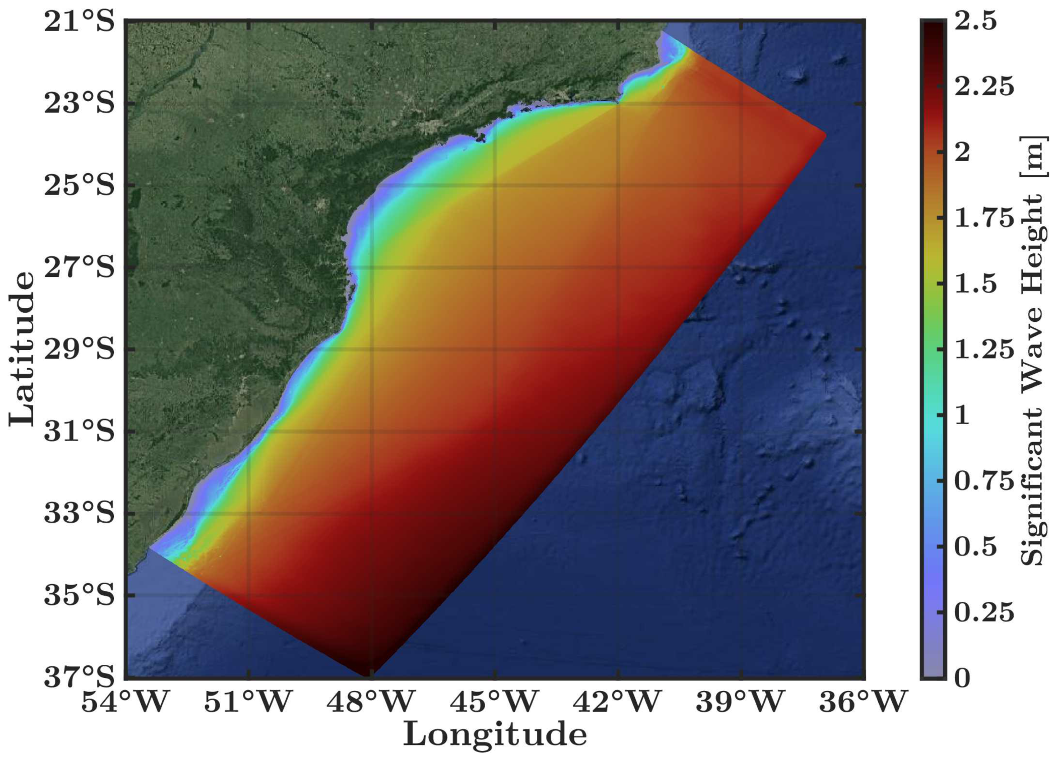
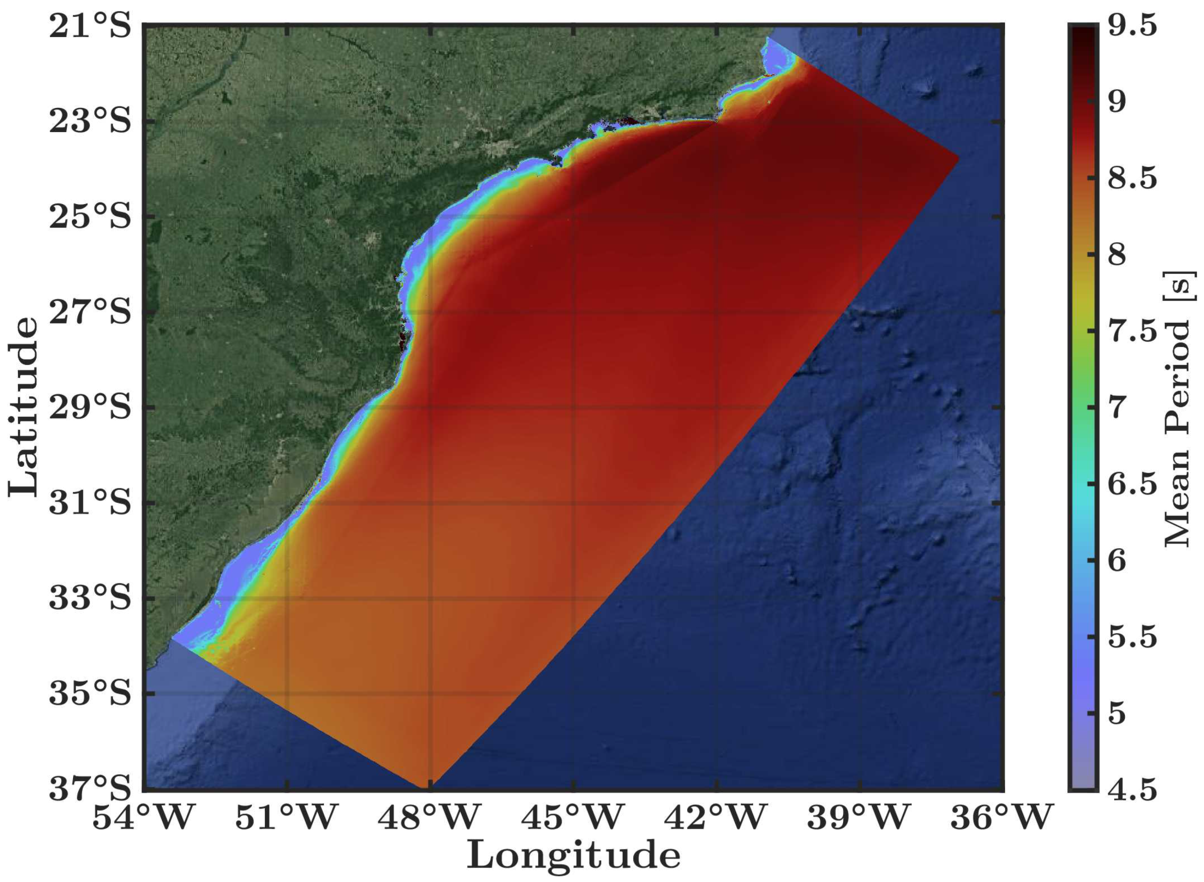
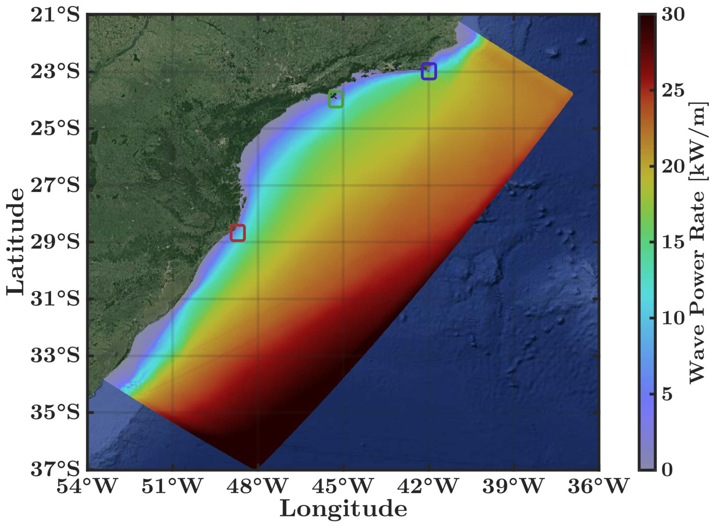
3.1. Temporal Mean Analysis

To obtain initial insight into the available resource of wave energy on the SSBS, the temporal mean of the modelled result was extracted over the entire studied region to calculate the mean surfaces of the calculated parameters. The mean Hs (Figure 5) shows similar behaviour along all of the SSBS, with values approximately 1.6 m over the continental shelf and reaching up 2.5 m in the oceanic region.
The mean Hs surface shows a discontinuity on the Santos Basin, with a gap within 1.5 m to 1.7 m , which begins at Farol Island (42° W, 23° S). This occurs because the island retains a part of the waves that propagate to the southwest, contributing to a decrease of Hs in the Santos Basin.
Southwest of the domain, the region of the Rio Grande do Sul coast (30° S to 34° S) has small wave amplitudes that are approximately 0.6 m . These smaller wave amplitudes appear to be the result of the mildly sloping beaches in this area [52]. Mildly sloped beaches dissipate much of the wave energy and do not allow greater wave heights to occur in this region.
The first exception to this pattern occurs on the coast of Laguna (48.74° W, 28.58° S), located in the Santa Catarina State, which has a mean Hs of 1.3 m near shore. Florianópolis (48.47° W, 27.70° S), a few kilometres to the north, has mean values lower than Laguna (approximately 1.1 m ).
Florianópolis is also the southern limit of the Santos Basin that at its southern portion presented the lowest mean values of Hs on the SSBS. The values are lower than 0.4 m , due to the extremely long continental shelf. In the middle part of the Santos Basin, near the São Paulo State, the Ilhabela island (45.21° W, 24° S) has the highest mean Hs of approximately 1.2 m . This value likely stems from the projection of Ilhabela towards the ocean.
The next remarkable location is Farol Island, near Arraial do Cabo city, which has the highest mean Hs of all of the studied coastlines (up to 1.6 m ), which is also due to its projection towards the ocean.
Tomawac determines the wave propagation direction based on the direction of the waves relative to true north in a clockwise direction [36]. The mean Dm surface (Figure 6) shows that the main direction of propagation of the waves is 235° (waves going to southwest), with a deflection eastward in the direction of the ocean (180°) and another deflection to the northwest (315°), perpendicular to the shoreline. This latter deflection appears to be due to the refraction of the waves.
This behaviour of waves, going to the southwest, complements the discontinuity found in the mean Hs surface. The waves arrive at Farol Island with a mean Dm of 230° and are blocked by the island, thereby reducing the Hs of the waves that arrive at the Santos Basin.
The mean surface of Tm (Figure 7) shows waves with periods between 8 s 9 s on the south and southeastern regions, respectively. These values are practically constant for the entire SSBS, except near the coastline, where it is possible to observe regions where the waves begin to be affected by the bottom. In these regions, the Tm lowers to 5 s , and wave height and length decrease.
The location of this variation is where dissipative processes are the least pronounced. These locations are Laguna, Ilhabela, and Farol Island. This finding leads to the prediction that these locations experience the most energetic waves on the SSBS.
Finally, the mean Pw field (Figure 8) exhibits the same behaviour as Hs because the wave energy is proportional to the square of the amplitude and the period [1]. The mean Pw in this oceanic region is approximately 22 kW / m and reaches up to 30 kW / m in the southern part of the domain. These elevated mean values in the southern region, for both Pw and Hs, are due to the wind fetch needed for the waves to develop in the Antarctic Ocean [1,17].
The wave energy is close to zero at locations very near the coastline on the southernmost part of the SSBS and in the Santos Basin. On the other hand, the most elevated values were observed in Laguna and Ilhabela, with 10 kW / m and Farol Island, with a mean value that reach up to 15 kW / m . Generally, the mean values simulated by the Tomawac model were quite similar to the Brazilian wave energy described by Pianca et al. [26].

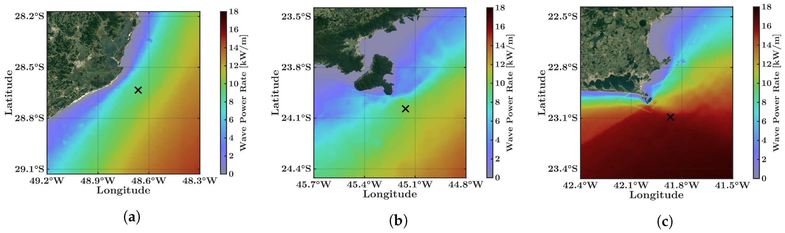
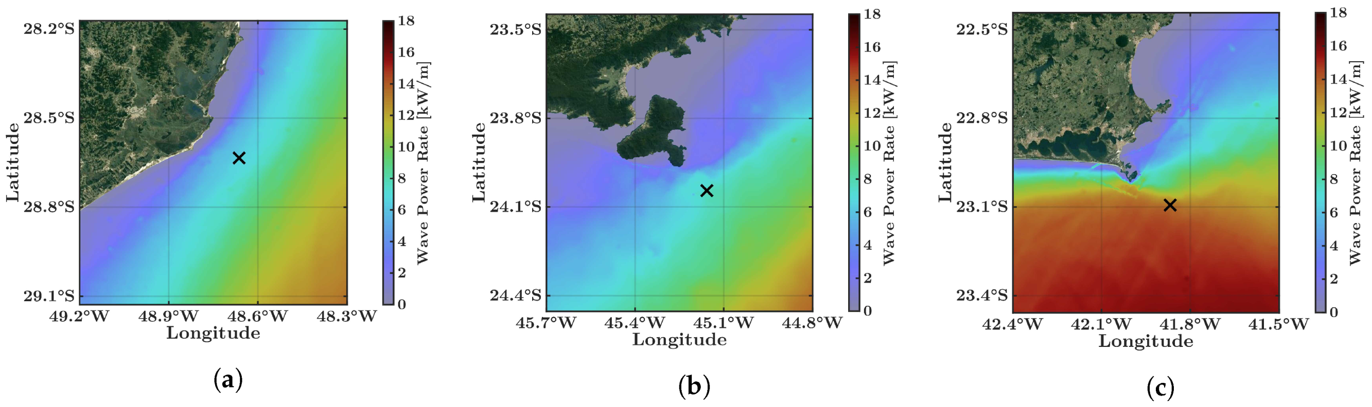
3.2. Local Wave Power Analysis

The installation of wave energy converters should be made as near the coast as possible to reduce costs during construction and operational periods. Therefore, installation could be conducted at the most energetic locations: Laguna, Ilhabela and Farol Island.
An analysis of the Pw available for conversion was conducted in the area of study. The selected locations are highlighted in Figure 8. A colormap of each location is presented in Figure 9.
The southernmost point in the coastal region is located near the city of Laguna. This point, located approximately 7 km from the coast has a mean Hs of 1.2 m (Figure 5), a relatively high value compared to other locations along the southern Brazilian coast.
The Pw spatial mean around Laguna (Figure 9a) exhibits an approximately linear behaviour parallel to the shoreline. This characteristic, combined with the bent geometry of the beach, contributes to the elevated mean Pw of this location.
Its mean surface shows that, of the entire coastline, the potential is higher perpendicular to the coast of the Santa Marta Cape. Examining the value of Pw from the coastline towards the ocean, a substantial increase from 2.0 kW / m to 7.0 kW / m within the first 4 km , and a subtle rise up to 10.0 kW / m within 20 km .
An important aspect of Pw is its temporal variability. Locations with smaller means and low variability are more efficient for energy conversion than locations with higher means and high variability. Neill and Hashemi [18], for instance, studied Great Britain, which has one of the highest Pw in the world. in Great Britain is more than 60 kW / m , which is unevenly distributed between the winter (up to 110 kW / m in average) and summer (close to zero).
Laguna, on the other hand, does not provide Pw as high as Great Britain but, in terms of variability, is far more stable. Temporal variability in Laguna is expressed in terms of standard deviation in Figure 10a. The general characteristics of the standard deviation are rather similar to those of the mean surface.
In the first few kilometres, there is a smaller increase in the standard deviation, from 1.5 kW / m to 4.5 kW / m , than in the mean power. Further away, there is a standard deviation of 8 kW / m , associated with a higher average of 10 kW / m . Thus, the suitability, based on mean values, is better in the first 5 km off the coastline.
In contrast with the linear behaviour of the waves mentioned above, Ilhabela has completely different wave characteristics on each side (Figure 9b). The southwestern sector offers a starting mean Pw of 4.5 kW / m on the first 2 km off the coastline and does not show considerable growth further away. The standard deviation (Figure 10b) of this sector exhibits the same behaviour as the mean power, starting at 3 kW / m but with slightly less growth advancing towards Santos Basin.
The northeastern side of Ilhabela has averages (Figure 9b) close to 1.75 kW / m near shore, which grow linearly to approximately 4 kW / m within 6 km from the coast. Despite being lower than the values found on the opposite side of the island, these are compensated by the lower standard deviation (Figure 10b) of 1.4 kW / m near the shore, which increase up to 2 kW / m further into the ocean.
The northeastern sector has steady mean values in the area that covers the inner continental shelf from 5 km to 10 km off the coast. Again, the standard deviation behaves similarly to the mean power but with a magnitude 1.5 to 1.8 times smaller.
The northernmost site selected was Farol Island, near Arraial do Cabo, in the Rio de Janeiro State. The entire region is located in a peninsula. Furthermore, Farol Island is projected towards the ocean, which makes dissipative processes much less effective on the waves that arrive to the island.
The mean Pw (Figure 9c) immediately south of the island is 15 kW / m , with an almost insignificant growth up to 17 kW / m , away from the island going south. At the eastern part of the island, the mean Pw is reduced to 12 kW / m at approximately 1 km off the coast. This value is constant further away into the sea. The behaviour is similar on the western side.
The standard deviation at these locations is fairly high (Figure 10c), but the high values are a consequence of high mean values. At the southern end of Farol Island, the standard deviation is 11 kW / m immediately beside the coastline, increasing up to 15 kW / m further towards the sea. The east side has a standard deviation of 7 kW / m and this value remains constant and similar to the mean values. The West sector, on the other hand, has a standard deviation of 11 kW / m .
Another notable location is the bay in between Farol Island and Armação dos Búzios ( 41.9 W, 22.72 S), located at approximately 10 km off the shoreline. This spot has the largest mean values compared to the standard deviation, twice as large in some locations. However, the mean power varies by approximately 7 kW / m and the standard deviation decreases to 3 kW / m .

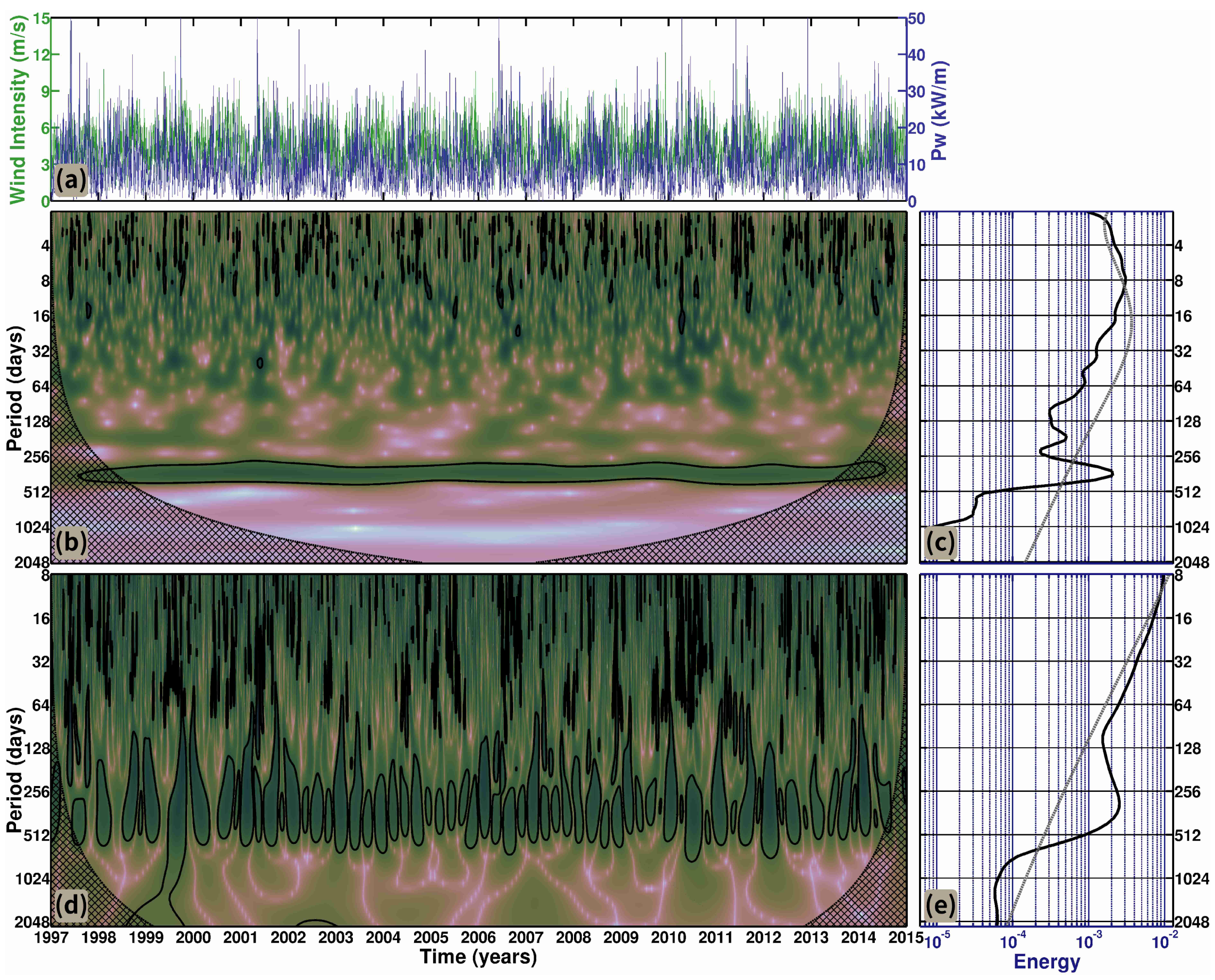
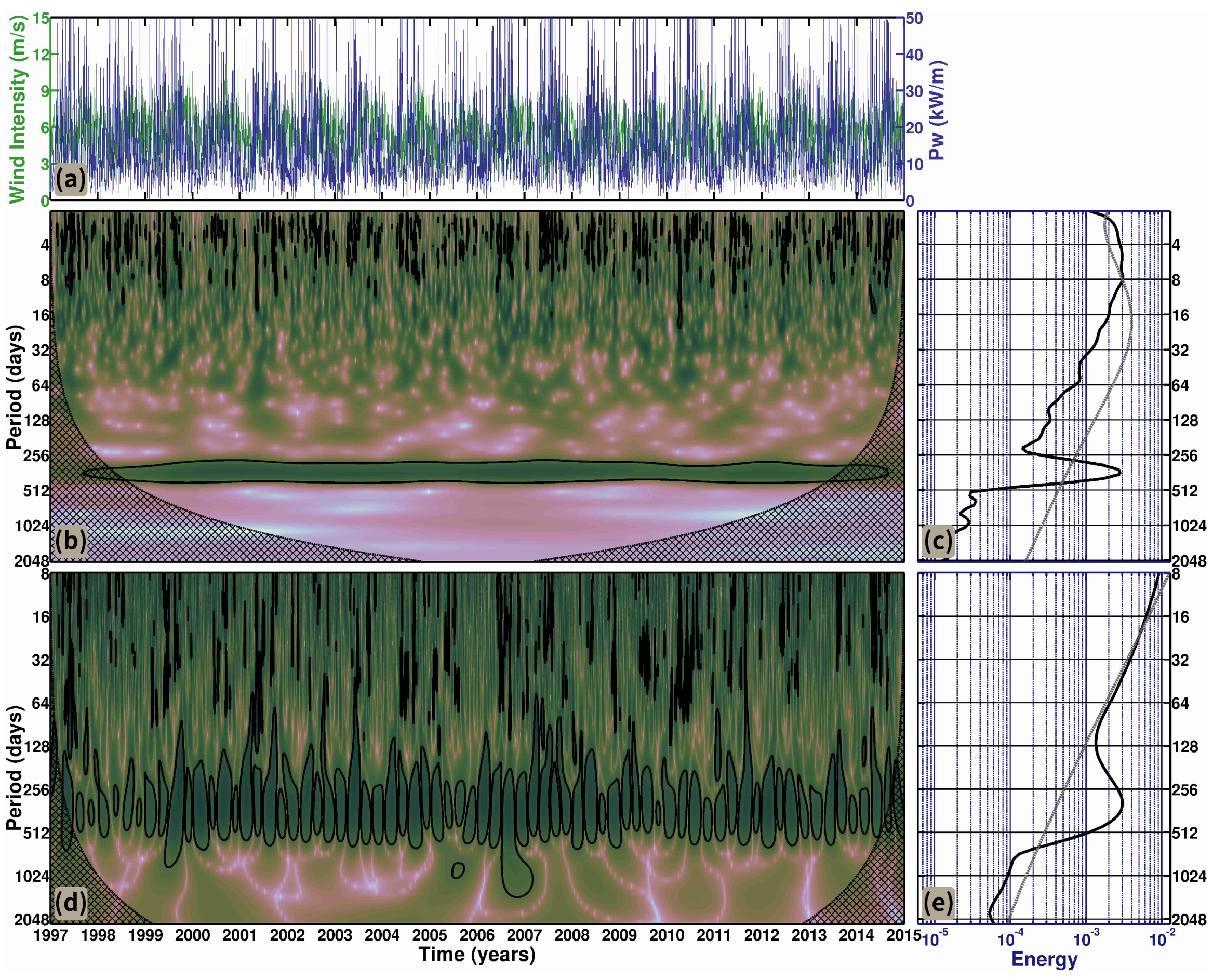
3.3. Temporal Variability

To investigate patterns in temporal variability of the three selected sites, Cross-Wavelet analysis was conducted according to the method of Torrence and Compo [50] and Liu [51]. This analysis consists of the deconstruction of two time series in frequency ranges and the correlation of both decomposed series with each other to detect similarities in variability patterns of their respective periods.
The time series used for comparisons were extracted from points approximately 15 km away from the coastline of all the three studied sites (“X” in Figure 9 and Figure 10). The wavelets were used to correlate the waves Pw with the wind intensity.
Figure 11a shows both extracted times series on Laguna. Pw ranged from zero to 21.5 kW / m and the wind intensity ranged from 1.1 m / s to 8.1 m / s . Figure 11b illustrates the Morlet local wavelet spectrum for Laguna: the most energetic frequencies are shown in dark red. The black outline encloses the parts of the spectrum that have 95% statistical confidence, while the regions below the dashed line are the regions where the border effects are present in the time series.
The Morlet local wavelet on Laguna (Figure 11b) shows a dominant annual cycle, which is existent for nearly the entire time series. Minor influences occur in 2004 and 2009, which indicates that there is variability in periods of 12–16 months. The local spectrum also shows synoptic variability with stronger effects during 2–7 days associated with the passage of meteorological systems.
Figure 11c presents the time-averaged Morlet local spectrum (global spectrum) on the frequency domain (black continuous line) and the 95% significance level (gray dashed line). The global spectrum has two dominant period ranges, indicating that synoptic variability is embedded in a more energetic annual cycle on the Pw available on Laguna.
The Mexican Hat local wavelet spectrum on Laguna (Figure 11d) shows predominance of the annual cycle and details the oscillatory pattern over time. Oscillations happen twice a year and indicate that a well-defined cycle lasts six months, thereby implying that winter–summer variation exists.
The mid-section of the local spectrum covers the annual cycle and extends itself to approximately 600 days (two years), which corresponds to variability in the El Niño Southern Oscillation (ENSO). The frequency of these oscillations ranges from occurrences every 1.5 years to less frequent oscillations. The first ENSO in the time series occurred in 1998, an extremely strong among the ENSO [53,54,55,56,57,58], followed by ENSO of 2002 [59,60], 2007 [61] and two events of smaller intensity in 2010 [62] and 2012, respectively. A time series with the Multivariate ENSO Index can be found at NOAA4.
Figure 11e shows the global spectrum for the Mexican Hat wavelet and three distinct time scales are dominant. The shortest and less energetic is the 15 to 30 days oscillation, followed by the intra-seasonal time scales and the most energetic annual cycle. Again, this is the most important fraction of the spectrum. The Mexican Hat wavelet also shows that the ENSO plays a significant role in the energy spectrum of this location.
Moving on to Ilhabela, Figure 12a shows Pw in the interval between zero and 24.6 kW / m and wind intensity from 1.0 m / s to 7.7 m / s . The Morlet local wavelet spectrum (Figure 12b) shows a well-defined presence of an annual cycle along the entire time series associated with the largest part of the global spectrum (Figure 12c).
The dominant cycle observed for Ilhabela on the Mexican Hat Wavelet (Figure 12d) is also the yearly cycle [63], which holds most of the energy spectrum. This is primarily due to the well-defined seasonality of this region [63,64]. Associated with the annual pattern, there are cycles with considerable influence from 6 to 18 months, the former being associated with the seasonal pattern and the latter with short-term ENSO influence.
Gan and Rao [64] analysed cyclogenesis frequency for several years on the South American coast and showed a strong tendency for cyclone generation during the winter and a weaker tendency during the summer, with the autumn and spring being transitional seasons. Because cyclones have a direct effect on wind-driven waves, this difference between seasons is certainly one source of the yearly variability patterns in waves.
Different from Laguna, the annual cycle in Ilhabela has four oscillations within one year, which implies that there is a distinct behaviour in each season. This seasonal behaviour can also be observed on the global spectrum (Figure 12e), which shows much stronger seasonal variability in Ilhabela than in Laguna. This pattern accounts for a significant part of the Ilhabela energy spectrum.
The longer period events are weaker on Ilhabela, with a single episode on the local spectrum (Figure 12d), corresponding to the previously mentioned ENSO of 1998 [53,54,55,56,57,58].
Finally, at Farol Island, there is a higher Pw (Figure 13a), with common values up to 42.0 kW / m , caused by the intense average winds in this region, between 1.7 m / s and 9.0 m / s . The high intensity of winds appear to be due to the greater influence of the of south Atlantic Anticyclone at middle latitudes over this island [65,66], thereby making Farol Island have the highest values of Pw in the study region.
The Morlet local wavelet spectrum on Farol Island (Figure 13b) shows a highly concentrated energy on the yearly cycles, with little spread to higher or lower frequency oscillations. The local spectrum also shows that, for this location, there are no cycles with periods between one and two weeks that limit the synoptic time scale oscillations to one week at most.
The global Morlet spectrum (Figure 13c) shows a peak of energy on the annual cycle and a decrease in synoptic variability. In addition, the Mexican Hat local wavelet spectrum on Farol Island (Figure 13d) displays the same narrow interval for the yearly cycle found on the Morlet spectrum. A pattern similar to that found on Ilhabela can be observed here, with four high energy cells within a year and less energetic patterns from 6 to 18 months.
The Morlet spectrum (Figure 13e) also shows that the two-week pattern is not observable on Farol Island. The shortest time scale captured by the Mexican Hat spectrum is a monthly pattern, which still has low energy.
In addition, the seasonal cycle also has little influence on the spectrum. On Ilhabela, the long period ENSO has a weak presence; on Farol Island, ENSO has a single occurrence in the four-year time scale, in between 2006 and 2007.
The results show that, over 18 years, Farol Island is more stable during the annual cycle. On the other hand, the less stable location is Laguna, which exhibits no pattern at all over time. A comparison can be performed between global energy spectra.
The global energy spectra (Figure 11c,e, Figure 12c,e and Figure 13c,e) show most of the energy located on the annual cycle for the three locations but, among the locations studied, the most energetic one is Farol Island, with 1.2 times more energy than Ilhabela and 1.9 times more than Laguna. Additionally, the Morlet global spectra (Figure 11c, Figure 12c, and Figure 13c) show that the yearly cycle has 23, 38 and 47 times more energy than the synoptic cycle on Laguna, Ilhabela and Farol Island, respectively.
Similarly, the Mexican Hat global spectra (Figure 11e, Figure 12e and Figure 13e) determined that there is 2.7, 3.6 and 4.3 times more energy for the annual cycle than there is for the seasonal and monthly cycles on Laguna, Ilhabela and Farol Island, respectively.
The mean Mexican Hat global energy spectra (Figure 11e, Figure 12e and Figure 13e) show a similar behaviour for the three sites for cycles from 8 to 650 days. For longer cycles, the behaviour becomes quite different. Laguna has the most energetic effect due to the long period (more than two years) ENSO, with three significant appearances within 18 years.
The annual cycle is dominant on the three spectra and the strongest was verified in Farol Island. The synoptic and seasonal patterns are stronger on Ilhabela and have about the same energy contribution on the Farol Island and Laguna.
Finally, Table 3 shows basic statistical parameters calculated for the Pw time series used on wavelet analysis. Corroborating previous results, all of the values calculated for the time series on Farol Island are substantially higher than those calculated for the other localities.
The mean Pw on Laguna and Ilhabela are similar, but Pw on Farol Island is approximately 65% higher. The same behaviour was observed in the standard deviation, but with a difference of approximately 90%.
The maximum values, on the other hand, showed the greatest difference between Laguna and Ilhabela, and less from Ilhabela to Farol Island. However, these peak values are single values in the time series and do not occur frequently enough to have a great impact on the final power output.
The most remarkable difference lies on the integrated values that show the similarities between Laguna and Ilhabela. The integrated value exhibits a 60% increase on Farol Island, with 209.5 MW / m .

4. Conclusions

The third generation model Tomawac was validated using a four-year simulation to analyse wave energetic potential. Afterwards, a case study simulation of 18 years, from 1997 to 2014 was conducted on the SSBS.
The temporal mean results of the simulation show a generally constant behaviour of wave parameters Hs, Tm, Dm and Pw on the oceanic region. As the waves approach the coastline, the Hs, Tm and Pw values decrease due to bottom friction, while the Dm undergoes the refraction effect and deflects towards the coast.
Three study sites were chosen based on the Hs and Pw parameters. The locations are Laguna, with a mean Hs of 1.3 m and Pw, with a mean of 10 kW / m ; Ilhabela, with mean Hs and Pw of 1.2 m and 10 kW / m , respectively; and Farol Island, with means of 1.6 m and 15 kW / m for Hs and Pw, respectively.
After selecting the study sites, Cross-Wavelet analysis was used on a time series of Pw and wind intensity to define the variability cycles for each location. The main variability cycle observed at the three locations is the annual cycle, which was present over the 18 years simulated, with a strong seasonal presence on Ilhabela. The synoptic cycles are, as expected, present at all localities but with little influence on Farol Island.
ENSO has an important role on wavelet spectra, appearing as relatively short-term oscillations ranging from 1.5 to 2 years. Long-term ENSO have a smaller influence on Ilhabela and a major influence on Farol Island. These appear as 5 to 10-year oscillations on Laguna and as high energy events on Farol Island, with periods lasting approximately 10 years.
Thus, the most feasible location found in this study for a hypothetical installation of wave energy converters is the region adjacent to Farol Island. Higher mean values were obtained at this location, in addition to the largest integrated values. In terms of variability, Farol Island has the least energetic synoptic cycles, meaning that there is greater stability over time. Most of the energy oscillation is due to the annual cycle and the long-term variability caused by ENSO.

Author Contributions

The individual contribution to this paper was performed throughout conceptualization, P.H.O., C.F., W.C.M. and E.d.P.K.; methodology, P.H.O. and J.C.; software, P.H.O., C.F. and W.C.M.; validation, P.H.O., C.F., W.C.M. and E.d.P.K.; formal analysis, P.H.O. and J.C.; investigation, P.H.O., C.F. and W.C.M.; resources, W.C.M.; data curation, P.H.O., C.F., W.C.M., and E.d.P.K.; writing—original draft preparation, P.H.O., C.F. and W.C.M.; writing—review and editing, J.C. and E.d.P.K.; visualization, P.H.O.; supervision, W.C.M. and E.d.P.K.; project administration, W.C.M.; funding acquisition, W.C.M. and C.F.

Funding

This study was financed in part by the Coordenação de Aperfeiçoamento de Pessoal de Nível Superior—Brasil (CAPES)—Finance Code 001.

Acknowledgments

The authors are grateful to the Conselho Nacional de Desenvolvimento Científico e Tecnológico (CNPq) under contract 304227/2016-1 and to the Agência Nacional do Petróleo (ANP) regarding the Programa de Recursos Humanos (PRH–27) for the fellowships. The authors are also grateful to the Fundação de Amparo à Pesquisa do Estado do Rio Grande do Sul (FAPERGS) for sponsoring this research under the contracts 17/2551-001159-7, to the Coordenação de Aperfeiçoamento de Pessoal de Nível Superior (CAPES) for bursaries related to the Programa Nacional de Pós Doutorado. Additional acknowledgement goes to the Brazilian Navy for providing detailed bathymetric data for the coastal area, to NOAA for supplying the wind and wave datasets, and to Électricité de France (EDF) for the public licence for the Open Telemac-Mascaret system. A special thanks to the Supercomputing Center of the Federal University of Rio Grande do Sul (CESUP-UFRGS) and to the Sdumont Supercomputer from the Laboratório Nacional de Computação Científica (LNCC) (SDUMONT-2017-C01#166515) where most of the computational work was carried out.

Conflicts of Interest

The authors declare no conflict of interest.

Abbreviations

The following abbreviations are used in this manuscript:
ANPAgência Nacional do Petróleo
CAPESCoordenação de Aperfeiçoamento de Pessoal de Nível Superior
CESUP-UFRGSSupercomputing Center of the Federal University of Rio Grande do Sul
CNPqConselho Nacional de Desenvolvimento Científico e Tecnológico
ECMWFEuropean Centre for Medium-Range Weather Forecasts
EDFÉlectricité de France
ENSOEl Niño Southern Oscillation
FAPERGSFundação de Amparo à Pesquisa do Estado do Rio Grande do Sul
LNCCLaboratório Nacional de Computação Científica
NOAANational Oceanic and Atmospheric Administration
NCEPNational Centers for Environmental Prediction
NCARNational Center for Atmospheric Research
PNBOIAPrograma Nacional de Boias
PRHPrograma de Recursos Humanos
RMSERoot Mean Square Error
SIScatter Index
SSBSSouth-Southeastern Brazilian Shelf
TomawacTelemac-Based Operational Model Addressing Wave Action Computation
WAMWAve Model

References

  1. Clément, A.; McCullen, P.; Falcão, A.; Fiorentino, A.; Gardner, F.; Hammarlund, K.; Lemonis, G.; Lewis, T.; Nielsen, K.; Petroncini, S.; et al. Wave energy in Europe: Current status and perspectives. Renew. Sustain. Energy Rev. 2002, 6, 405–431. [Google Scholar] [CrossRef]
  2. López, I.; Andreu, J.; Ceballos, S.; Alegría, I.M.D.; Kortabarria, I. Review of wave energy technologies and the necessary power-equipment. Renew. Sustain. Energy Rev. 2013, 27, 413–434. [Google Scholar] [CrossRef]
  3. Jama, M.A.; Noura, H.; Wahyudie, A.; Assi, A. Enhancing the performance of heaving wave energy converters using model-free control approach. Renew. Energy 2015, 83, 931–941. [Google Scholar] [CrossRef]
  4. Buccino, M.; Stagonas, D.; Vicinanza, D. Development of a composite sea wall wave energy converter system. Renew. Energy 2015, 81, 509–522. [Google Scholar] [CrossRef]
  5. Bódai, T.; Srinil, N. Performance analysis and optimization of a box-hull wave energy converter concept. Renew. Energy 2015, 81, 551–565. [Google Scholar] [CrossRef]
  6. Gaspar, J.F.; Calvário, M.; Kamarlouei, M.; Guedes Soares, C. Power take-off concept for wave energy converters based on oil-hydraulic transformer units. Renew. Energy 2016, 86, 1232–1246. [Google Scholar] [CrossRef]
  7. Rusu, E. Evaluation of the wave energy conversion efficiency in various coastal environments. Energies 2014, 7, 4002–4018. [Google Scholar] [CrossRef]
  8. Carballo, R.; Sánchez, M.; Ramos, V.; Fraguela, J.A.; Iglesias, G. Intra-annual wave resource characterization for energy exploitation: A new decision-aid tool. Energy Convers. Manag. 2015, 93, 1–8. [Google Scholar] [CrossRef]
  9. Robertson, B.; Hiles, C.; Luczko, E.; Buckham, B. Quantifying wave power and wave energy converter array production potential. Int. J. Mar. Energy 2016, 14, 143–160. [Google Scholar] [CrossRef]
  10. Cahill, B.G.; Lewis, T. Wave energy resource characterisation of the Atlantic Marine Energy Test Site. Int. J. Mar. Energy 2013, 1, 3–15. [Google Scholar] [CrossRef]
  11. Kim, J.; Kweon, H.M.; Jeong, W.M.; Cho, I.H.; Cho, H.Y. Design of the dual-buoy wave energy converter based on actual wave data of east sea. Int. J. Naval Archit. Ocean Eng. 2015, 7, 739–749. [Google Scholar] [CrossRef]
  12. Yaakob, O.; Hashim, F.E.; Mohd Omar, K.; Md Din, A.H.; Koh, K.K. Satellite-based wave data and wave energy resource assessment for South China Sea. Renew. Energy 2016, 88, 359–371. [Google Scholar] [CrossRef]
  13. Isaacs, J.D.; Seymour, R.J. The Ocean as a Power Resource. Int. J. Environ. Stud. 1973, 4, 201–205. [Google Scholar] [CrossRef]
  14. Krogstad, H.E.; Barstow, S.F. Satellite wave measurements for coastal engineering applications. Coast. Eng. 1999, 37, 283–307. [Google Scholar] [CrossRef]
  15. Arinaga, R.A.; Cheung, K.F. Atlas of global wave energy from 10 years of reanalysis and hindcast data. Renew. Energy 2012, 39, 49–64. [Google Scholar] [CrossRef]
  16. Reguero, B.G.; Losada, I.J.; Méndez, F.J. A global wave power resource and its seasonal, interannual and long-term variability. Appl. Energy 2015, 148, 366–380. [Google Scholar] [CrossRef]
  17. Gunn, K.; Stock-Williams, C. Quantifying the global wave power resource. Renew. Energy 2012, 44, 296–304. [Google Scholar] [CrossRef]
  18. Neill, S.P.; Hashemi, M.R. Wave power variability over the northwest European shelf seas. Appl. Energy 2013, 106, 31–46. [Google Scholar] [CrossRef]
  19. Stopa, J.E.; Cheung, K.F.; Chen, Y.l. Assessment of wave energy resources in Hawaii. Renew. Energy 2011, 36, 554–567. [Google Scholar] [CrossRef]
  20. Iglesias, G.; Carballo, R. Wave resource in El Hierro-an island towards energy self-sufficiency. Renew. Energy 2011, 36, 689–698. [Google Scholar] [CrossRef]
  21. Liang, B.; Fan, F.; Yin, Z.; Shi, H.; Lee, D. Numerical modelling of the nearshore wave energy resources of Shandong peninsula, China. Renew. Energy 2013, 57, 330–338. [Google Scholar] [CrossRef]
  22. Hiles, C.E.; Buckham, B.J.; Wild, P.; Robertson, B. Wave energy resources near Hot Springs Cove, Canada. Renew. Energy 2014, 71, 598–608. [Google Scholar] [CrossRef]
  23. Robertson, B.R.D.; Hiles, C.E.; Buckham, B.J. Characterizing the near shore wave energy resource on the west coast of Vancouver Island, Canada. Renew. Energy 2014, 71, 665–678. [Google Scholar] [CrossRef]
  24. Hemer, M.A.; Griffin, D.A. The wave energy resource along Australia’s Southern margin. J. Renew. Sustain. Energy 2010, 2, 1–15. [Google Scholar] [CrossRef]
  25. Behrens, S.; Hayward, J.; Hemer, M.; Osman, P. Assessing the wave energy converter potential for Australian coastal regions. Renew. Energy 2012, 43, 210–217. [Google Scholar] [CrossRef]
  26. Pianca, C.; Mazzini, P.L.F.; Siegle, E. Brazilian offshore wave climate based on NWW3 reanalysis. Braz. J. Oceanogr. 2010, 58, 53–70. [Google Scholar] [CrossRef]
  27. Parise, C.K.; Farina, L. Ocean wave modes in the South Atlantic by a short-scale simulation. Tellus A 2012, 64, 1–14. [Google Scholar] [CrossRef]
  28. Losada, I.J.; Reguero, B.G.; Méndez, F.J.; Castanedo, S.; Abascal, A.J.; Mínguez, R. Long-term changes in sea-level components in Latin America and the Caribbean. Glob. Planet. Chang. 2013, 104, 34–50. [Google Scholar] [CrossRef]
  29. Guimarães, P.V.; Farina, L.; Toldo, E.E., Jr. Analysis of extreme wave events on the southern coast of Brazil. Nat. Hazards Earth Syst. Sci. 2014, 14, 3195–3205. [Google Scholar] [CrossRef]
  30. Guimarães, P.V.; Farina, L.; Toldo, E.E., Jr.; Diaz-Hernandez, G.; Akhmatskaya, E. Numerical simulation of extreme wave runup during storm events in Tramandaí Beach, Rio Grande do Sul, Brazil. Coast. Eng. 2015, 95, 171–180. [Google Scholar] [CrossRef]
  31. Cuchiara, D.; Fernandes, E.; Strauch, J.; Winterwerp, J.; Calliari, L. Determination of the wave climate for the southern Brazilian shelf. Cont. Shelf Res. 2009, 29, 545–555. [Google Scholar] [CrossRef]
  32. Parente, C.E.; Nogueira, I.C.M.; Martins, R.P.; Ribeiro, E.O. Climatologia de Ondas. In Caracterização Ambiental Regional da Bacia de Campos, Atlântico Sudoeste: Meteorologia e Oceanografia. Habitats, 1st ed.; Martins, R.P., Santiago Grossmann-Matheson, G., Eds.; Elsevier: Rio de Janeiro, Brazil, 2015; Chapter 2; pp. 55–98. [Google Scholar]
  33. Green, D.A. A colour scheme for the display of astronomical intensity images. Bull. Astron. Soc. India 2011, 39, 289–295. [Google Scholar]
  34. Tolman, H.L. A Third-Generation Model for Wind Waves on Slowly Varying, Unsteady, and Inhomogeneous Depths and Currents. J. Phys. Oceanogr. 1991, 21, 782–797. [Google Scholar] [CrossRef]
  35. Komen, G.J.; Cavaleri, L.; Donelan, M.; Hasselmann, K.; Hasselmann, S.; Janssen, P.A.E.M. Dynamics and mOdelling of Ocean Waves; Cambridge University Press: Cambridge, UK, 1994; p. 532. [Google Scholar]
  36. Awk, T. Tomawac User Manual Version 7.2, Technical Report; The TELEMAC-Mascaret Consortium, Version 7.2.3. 2017.
  37. Tolman, H.L. User Manual and System Documentation of WAVEWATCH III Version 1.15; Technical Report; National Oceanic and Atmospheric Administration: Washington, DC, USA, 1997.
  38. Tolman, H.L. User Manual and System Documentation of WAVEWATCH III Version 1.18; Technical Report; National Oceanic and Atmospheric Administration: Washington, DC, USA, 1999.
  39. Tolman, H.L. User Manual and System Documentation of WAVEWATCH III Version 3.14; Technical Report; National Oceanic and Atmospheric Administration: Washington, DC, USA, 2009.
  40. Kalnay, E.; Kanamitsu, M.; Kistler, R.; Collins, W.; Deaven, D.; Gandin, L.; Iredell, M.; Saha, S.; White, G.; Woollen, J.; et al. The NCEP/NCAR 40-Year Reanalysis Project. Bull. Am. Meteorol. Soc. 1996, 77, 437–472. [Google Scholar] [CrossRef]
  41. Janssen, P.A.E.M.; Hansen, B.; Bidlot, J.R. Verification of the ECMWF Wave Forecasting System against Buoy and Altimeter Data. Am. Meteorol. Soc. 1997, 12, 763–784. [Google Scholar] [CrossRef]
  42. Lalbeharry, R. Evaluation of the CMC regional wave forecasting system against buoy data. Atmos. Ocean 2002, 40, 1–20. [Google Scholar] [CrossRef]
  43. Melo, E.; Hammes, G.R.; Franco, D.; Romeu, M.A.R. Avaliação de desempenho do modelo WW3 em Santa Catarina. In Proceedings of the Anais do III SEMENGO: Seminário e Workshop em Engenharia Oceânica, Rio Grande, Brazil, 2008. [Google Scholar]
  44. Melo, E.; Romeu, M.; Hammes, G. Condições extremas de agitação marítima ao largo de Rio Grande a partir do modelo WW3. In Proceedings of the Anais do IV Seminário e Workshop em Engenharia Oceânica, Rio Grande, Brazil, 2010; pp. 1–20. [Google Scholar]
  45. Chawla, A.; Spindler, D.M.; Tolman, H.L. Validation of a thirty year wave hindcast using the Climate Forecast System Reanalysis winds. Ocean Model. 2013, 70, 189–206. [Google Scholar] [CrossRef]
  46. Edwards, E.; Cradden, L.; Ingram, D.; Kalogeri, C. Verification within wave resource assessments. Part 1: Statistical analysis. Int. J. Mar. Energy 2014, 8, 50–69. [Google Scholar] [CrossRef]
  47. Dos Santos, R.B. Estudo Do Potencial Energético de Ondas Geradas pelo Vento para a Plataforma Continental sul do Brasil. Ph.D. Thesis, Universidade Federal do Rio Grande, Porto Alegre, Brazil, 2009. [Google Scholar]
  48. Iuppa, C.; Cavallaro, L.; Vicinanza, D.; Foti, E. Investigation of suitable sites for wave energy converters around Sicily (Italy). Ocean Sci. 2015, 11, 543–557. [Google Scholar] [CrossRef]
  49. Cavaleri, L. Wave Modeling—Missing the Peaks. Mar. Sci. 2009, 39, 2757–2778. [Google Scholar] [CrossRef]
  50. Torrence, C.; Compo, G.C. A Practical Guide to Wavelet Analysis. Bull. Am. Meteorol. Soc. 1998, 79, 61–78. [Google Scholar] [CrossRef]
  51. Liu, Y.; Liang, X.S.; Weisberg, R.H. Rectification of the bias in the wavelet power spectrum. J. Atmos. Ocean. Technol. 2007, 24, 2093–2102. [Google Scholar] [CrossRef]
  52. Martins, L.R.; Coutinho, P.N. The Brazilian continental margin. Earth-Sci. Rev. 1981, 17, 87–107. [Google Scholar] [CrossRef]
  53. Garcia-Herrera, R.; Barriopedro, D.; Hernández, E.; Diaz, H.F.; Garcia, R.R.; Prieto, M.R.; Moyano, R. A Chronology of El Niño Events from Primary Documentary Sources in Northern Peru. J. Clim. 2008, 21, 1948–1962. [Google Scholar] [CrossRef]
  54. Xu, K.M.; Wong, T.; Wielicki, B.A.; Parker, L. Statistical Analyses of Satellite Cloud Object Data from CERES. Part IV: Boundary Layer Cloud Objects 1998 El Niño. J. Clim. 2008, 21, 6668–6688. [Google Scholar] [CrossRef]
  55. Marques, W.; Fernandes, E.; Monteiro, I.; Möller, O. Numerical modeling of the Patos Lagoon coastal plume, Brazil. Cont. Shelf Res. 2009, 29, 556–571. [Google Scholar] [CrossRef]
  56. Marques, W.C.; Fernandes, E.H.L.; Moraes, B.C.; Möller, O.O.; Malcherek, A. Dynamics of the Patos Lagoon coastal plume and its contribution to the deposition pattern of the southern Brazilian inner shelf. J. Geophys. Res. Oceans 2010, 115, C10045. [Google Scholar] [CrossRef]
  57. Marques, W.C.; Fernandes, E.H.L.; Moller, O.O. Straining and advection contributions to the mixing process of the Patos Lagoon coastal plume, Brazil. J. Geophys. Res. 2010, 115, C06019. [Google Scholar] [CrossRef]
  58. Marques, W.C.; Fernandes, E.H.L.; Rocha, L.A.O. Straining and advection contributions to the mixing process in the Patos Lagoon estuary, Brazil. J. Geophys. Res. 2011, 116, C03016. [Google Scholar] [CrossRef]
  59. McPhaden, M.J. Evolution of the 2002/03 El Niño. Bull. Am. Meteorol. Soc. 2004, 85, 677–695. [Google Scholar] [CrossRef]
  60. Goddard, L.; Kumar, A.; Hoerling, P.P.; Barnston, A.G. Diagnosis of Anomalous Winter Temperatures over the Eastern United States during the 2002 / 03 El Niño. J. Clim. 2006, 19, 5624–5636. [Google Scholar] [CrossRef]
  61. Okumura, Y.M.; Deser, C. Asymmetry in the Duration of El Niño and La Niña. J. Clim. 2010, 23, 5826–5843. [Google Scholar] [CrossRef]
  62. Robinson, C.J.; Gómez-Gutiérrez, J.; Markaida, U.; Gilly, W.F. Prolonged decline of jumbo squid (Dosidicus gigas) landings in the Gulf of California is associated with chronically low wind stress and decreased chlorophyll a after El Niño 2009–2010. Fish. Res. 2015, 173, 128–138. [Google Scholar] [CrossRef]
  63. Busalacchi, A.J.; Picaut, J. Seasonal Variability from a Model of the Tropical Atlantic Ocean. J. Phys. Oceanogr. 1983, 13, 1564–1588. [Google Scholar] [CrossRef]
  64. Gan, M.A.; Rao, V.B. Surface Cyclogenesis over South America. Mon. Weather Rev. 1991, 119, 1293–1302. [Google Scholar] [CrossRef]
  65. Venegas, S.A.; Mysak, L.A.; Straub, D.N. Atmosphere-ocean coupled variability in the south atlantic. J. Clim. 1997, 10, 2904–2920. [Google Scholar] [CrossRef]
  66. Liebmann, B.; Kiladis, G.N.; Marengo, J.A.; Ambrizzi, T.; Glick, J.D. Submonthly convective variability over South America and the South Atlantic convergence zone. J. Clim. 1999, 12, 1877–1891. [Google Scholar] [CrossRef]
1.
2.
3.
4.
Figure 1. Study region on the south-southeastern Brazilian Shelf (a); and location of the wave buoys (b). Colour bars represent the bathymetry varying from 0 to 5000 m depth. Cube Helix color scheme developed by Green [33]. Satellite images from maps.google.com.
Jmse 07 00025 g001
Figure 2. Representation of the numerical grid used for the simulations. Satellite images from maps.google.com.
Jmse 07 00025 g002
Figure 3. Hs time series from Tomawac (black lines) and measured data (coloured dots) from the wave buoy located off the coast of: (top) Rio Grande do Sul; (middle) Santa Catarina; and (bottom) São Paulo (sampled at a three-hourly interval).
Jmse 07 00025 g003
Figure 4. Scatter plots of the buoy data (horizontal axis) vs. Tomawac’s result (vertical axis): (a) Rio Grande do Sul; (b) Santa Catarina; (c) São Paulo. The colour represents the number of data points in each bin. The solid line shows the linear regression of the data set and the dotted 45° line represents an ideal regression for comparison.
Jmse 07 00025 g004
Figure 5. Mean value of significant wave height Hs ( m ) over 18 years.
Jmse 07 00025 g005
Figure 6. Mean value of mean direction Dm ( ° ) over 18 years.
Jmse 07 00025 g006
Figure 7. Mean value of mean period Tm ( s ) over 18 years.
Jmse 07 00025 g007
Figure 8. Mean value of wave power rate Pw ( k W / m ) over 18 years. Selected regions are highlighted using a black rectangle (Laguna), white rectangle (Ilhabela) and red rectangle (Farol Island).
Jmse 07 00025 g008
Figure 9. Mean value of wave power rate Pw ( k W / m ) over the 18 years simulated. The “X” marks the position where the time series were extracted for the wavelet analysis in Section 3.3: (a) Laguna; (b) Ilhabela; and (c) Farol Island.
Jmse 07 00025 g009
Figure 10. Standard deviation of wave power rate Pw ( k W / m ) over the 18 years simulated. The “X” marks the position where the time series were extracted for the wavelet analysis in Section 3.3: (a) Laguna; (b) Ilhabela; and (c) Farol Island.
Jmse 07 00025 g010
Figure 11. (a) Time series of wind intensity (blue) and Pw (green) used for the cross-wavelet analysis. (b) Local Morlet wavelet power spectrum. Thick contour lines enclose regions of greater than 95% confidence for a red noise process with a lag 1 coefficient of 0.7. Cross-hatched regions indicate the cone of influence where edge effects become important. (c) Global Morlet power spectrum of the time series and the dotted line indicate the 95% confidence level. (d) Mexican Hat local wavelet power spectrum. Thick contour lines enclose regions of greater than 95% confidence for a red noise process with a lag 1 coefficient of 0.1. Cross-hatched regions indicate the cone of influence where edge effects become important and. (e) Global Mexican Hat power spectrum of the time series and the dotted line indicate the 95% confidence level on the coastal zone of Laguna. Cube Helix color scheme developed by Green [33].
Jmse 07 00025 g011
Figure 12. (a) Time series of wind intensity (blue) and Pw (green) used for the cross-wavelet analysis. (b) Local Morlet wavelet power spectrum. Thick contour lines enclose regions of greater than 95% confidence for a red noise process with a lag 1 coefficient of 0.7. Cross-hatched regions indicate the cone of influence where edge effects become important. (c) Global Morlet power spectrum of the time series and the dotted line indicate the 95% confidence level. (d) Mexican Hat local wavelet power spectrum. Thick contour lines enclose regions of greater than 95% confidence for a red noise process with a lag 1 coefficient of 0.1. Cross-hatched regions indicate the cone of influence where edge effects become important and. (e) Global Mexican Hat power spectrum of the time series and the dotted line indicate the 95% confidence level on the coastal zone of Ilhabela. Cube Helix color scheme developed by Green [33].
Jmse 07 00025 g012
Figure 13. (a) Time series of wind intensity (blue) and Pw (green) used for the cross-wavelet analysis. (b) Local Morlet wavelet power spectrum. Thick contour lines enclose regions of greater than 95% confidence for a red noise process with a lag 1 coefficient of 0.7. Cross-hatched regions indicate the cone of influence where edge effects become important. (c) Global Morlet power spectrum of the time series and the dotted line indicate the 95% confidence level. (d) Mexican Hat local wavelet power spectrum. Thick contour lines enclose regions of greater than 95% confidence for a red noise process with a lag 1 coefficient of 0.1. Cross-hatched regions indicate the cone of influence where edge effects become important. (e) Global Mexican Hat power spectrum of the time series and the dotted line indicates the 95% confidence level on the coastal zone of Farol Island. Cube Helix color scheme developed by Green [33].
Jmse 07 00025 g013
Table 1. Mathematical equations to compute the error metrics.
Root Mean Square Error RMSE = T i B i 2 n
Scatter Index S I = RMSE B ¯
Correlation Coefficient r = T i · B i n · T ¯ B ¯ T i 2 n · T ¯ 2 · B i 2 n · B ¯ 2
Table 2. Statistical parameters calculated using the measured buoy data (B) and the Tomawac output (T).
ParameterRio Grande
Do Sul
Santa
Catarina
São
Paulo
BTBTBT
HsAverage [ m ]2,061,801,941,772,011,81
Root Mean Square Error [ m ]0,580,500,61
Correlation Coefficient0,910,890,91
Scatter Index0,280,260,30
TpAverage [ s ]9,518,639,829,119,778,79
Root Mean Square Error [ s ]2,072,002,10
Correlation Coefficient0,930,920,93
Scatter Index0,220,200,22
Table 3. Statistical parameters calculated using the time series of each studied point over 18 years.
LagunaIlhabelaFarol Island
Mean [ kW / m ]9,0810,0115,93
Standard Deviation [ kW / m ]6,477,5913,51
Maximum [ kW / m ]79,88112,13140,70
Integrated [ MW / m ]119,36131,66209,50

