A Novel Obstacle Localization Method for an Underwater Robot Based on the Flow Field

Abstract

Because the underwater environment is complex, autonomous underwater vehicles (AUVs) have difficulty locating their surroundings autonomously. In order to improve the adaptive ability of AUVs, this paper presents a novel obstacle localization strategy based on the flow features. Like fish, the strategy uses the flow field information directly to locate the object obstacles. Two different localization methods are provided and compared. The first method, which is named the Method of Spatial Distribution (MSD), is based on the spatial distribution of the flow field. The second method, which is named the Method of Amplitude Variation (MAV), is provided by the amplitude variation of the flow field. The flow field around spherical targets is obtained by a numerical method, and both methods use the parallel velocity component on the virtual lateral line. During the study, different target numbers, detective ratios, spacing ratios, and flow velocities are taken into account. It is demonstrated that both methods are able to locate object obstacles. However, the prediction accuracy of MAV is higher than that of MSD. That implies that MAV is more robust than MSD. These new findings indicate that the object obstacles can be directly located based on the flow field information and robust flow sensing is perhaps not based on the spatial distribution of the flow field but rather, on its fluctuation range.

1. Introduction

The autonomous underwater vehicle (AUV) is an important piece of equipment that is used to explore the ocean. However, the adaptive ability of the AUV is poor because the underwater environment is complex. In order to improve its environmental adaptability, studies have mainly focused on its control strategy [1,2,3]. However, the AUV is still not as adaptable as fish. One main reason for this is that the AUV has difficulty sensing its surroundings autonomously. Conventionally, electromagnetic sensors, sonars, and vision sensors are applied for perception. They can offer numerous advantages to help AUV localization, but their usage is also limited for a variety of reasons. For example, the sonars locate object obstacles based on the emission of sound waves, a process which has high energy consumption. Moreover, their medium to low resolution and high cost is the main limitation of their usage in underwater localization. In addition, the electromagnetic waves attenuate faster in seawater [4]. The vision sensors are overly dependent on light conditions, resulting in a greater power requirement and a limited operating scope [5,6,7]. Despite the exploitation of electromagnetic sensors, sonars, and vision sensors for successful object obstacle avoidance by underwater robots, the new method has obvious room for development because of the limitations.

Recently, some studies have proven that flow sensing can provide useful information about an AUV’s surroundings [8,9]. Flow sensing has no relationship with illumination and noise conditions, and it can provide exteroceptive information in extreme environments [8,10,11]. The research on flow sensing based on lateral line mechanism can be divided into two parts. One is the study of ichthyology, and the other one is hydrodynamics.

Ichthyology mainly focuses on the structure of lateral organs and the behavior of fish after being stimulated. Based on the biologists’ studies of the lateral line system [12,13,14], some researchers have designed many artificial lateral line sensors. Such designs employ a variety of sensing principles, such as piezoresistive [15], capacitive [16], thermal [17], magnetic [18], piezoelectric [19], and optical techniques [20]. Hydrodynamics mainly focuses on the characteristics of the flow field around the target [21,22,23,24]. Research methods mainly include theoretical analysis and numerical simulations. Among the theoretical analysis methods, the potential flow theory has been used widely [25,26,27]. However, the potential flow theory is based on the assumption of idealized fluid, and the details of the flow field cannot be described accurately. With the development of computer technology, computational fluid dynamics (CFD) has become the main hydrodynamics method [28,29,30,31,32,33]. Based on these studies, we determined the structures of neuromasts and the flow fields around different targets. Because there is a wide academic gap between the ichthyology and hydrodynamics, we cannot determine the mechanism of the lateral line system used by the fish. For example, the specific stimuli information obtained by fish and the sensing processes based on this information are unknown. If we cannot build a bridge between ichthyology and hydrodynamics, the AUV will not be able to use lateral line sensors (LLS) to sense the environment [34].

In recent years, flow sensing has been introduced into the detection of objects. However, the most common method is the detection and localization of the dipole source [35,36,37]. One main method is the detection of Karman vortex streets (KVS) [38,39]. Another technique is the study of multisignal fusion and detection algorithms, which are based on the neural network scheme and other algorithms [40,41]. However, the excessive computing and storage resources and the difficulty of using these approaches for system level implementation mean that they cannot be used in engineering.

In this paper, we present a new flow sensing method for target localization. The relationship between the flow features and object location is investigated. The complete localization technique only uses flow velocity data as input parameters, and this technique has never been reported. This novel obstacle localization strategy uses the spatial distribution and amplitude variation of the flow field as flow features. An extensive comparative analysis between the two methods is carried out. The evaluation aims to study the differences between the methods—the Method of Spatial Distribution (MSD) and the Method of Amplitude Variation (MAV). The ultimate goal is to find a simple and effective method to locate the object obstacles based on the flow features.

The paper is organized as follows: Section 2 describes the background of the system model and the numerical method used to obtain the flow field, and the validation of numerical method is also described in this section. The novel object localization strategy is described in Section 3, including descriptions of MSD and MAV. Additionally, when the detective ratio changes, a comparison between two methods is provided. Section 4 presents the case of two tandem targets and the evaluation results of the two methods when the spacing ratio and flow velocity change. Finally, concluding remarks and directions for future work are provided in Section 5.

2. Implementation of the Test Problem

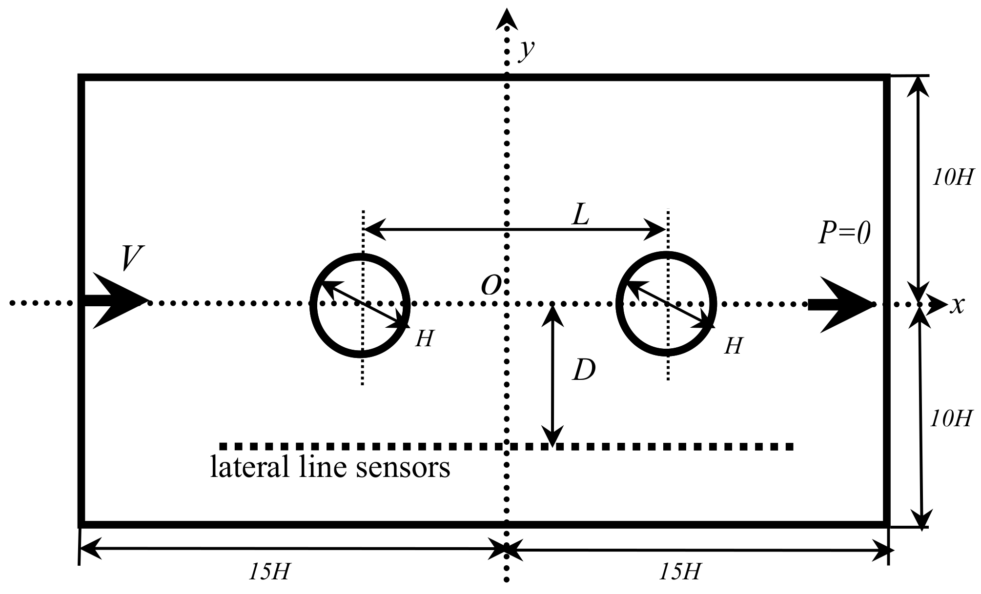
2.1. System Model

The lateral line and the targets are located in a Cartesian coordinate. As depicted in Figure 1, the diameter of the target is $H$. In order to avoid the influence of the computational domain on the flow field around the targets, the size of the computation field is 10 times larger than the target. Because the two targets are arranged in tandem and in order to ensure the full development of the wake field, the size of computation field along the flow direction is 30 times larger than the target. Thus, the computational domain $\mathsf{\Omega }$ is $30H\times 10H\times 10H$. In the case of two targets, $L$ is the distance between them. The lateral line is under the center of the targets, and the interval between two LLS is $0.01H$. The influence of the LLS is negligible. The sensors are located at $\left(x_i,y_i,z_i\right)$, and their range is shown in Equation (1):

$$\left\{\begin{array}{l}-12H\le x_i\le 12H;\\ y_i=-D;\\ z_i=0.\end{array}\right.,$$

(1)

where $H$ is the diameter of the target and $D$ is the detective distance.

At the inlet boundary, a uniform flow is prescribed to be $V$. The outlet condition is a pressure outlet, and the initial pressure is zero. A no-slip boundary is set as the surface of the targets, and a symmetry condition is used on the lateral boundaries. In order to ensure that the dynamic characteristics between the fluid and targets can be embodied accurately, the computational domain is defined by $\mathsf{\Omega }={\mathsf{\Omega }}_i+{\mathsf{\Omega }}_e$. The domain ${\mathsf{\Omega }}_i$ is the vicinity of targets, whose size is $24H\times 8H\times 8H$. The lateral lines used in this paper are located in this domain. Its grids are presented by employing an unstructured, triangular, and refined grid, whose size is $\Delta \chi$. Restricted by the computer resources, a grid increasing function is used to mesh the domain ${\mathsf{\Omega }}_e$ by a hexahedral grid. The surfaces of domain ${\mathsf{\Omega }}_i$ are used as the source, with an increasing ratio of 1.2 and a maximum size of $0.05H$.

To ensure the solution’s convergence, grid independence is studied. Three cases of the mesh dependency test are provided. When the residual is smaller than $1\times {10}^{-6}$, the solution can be seen as convergent. The minimum sizes $\Delta {\chi }_{\min }$ of the three cases are $0.001H$, $0.005H$, and $0.01H$, respectively. The drag coefficient $C_d$ and its percentage changes are shown in

Table 1. Analysis of grid independence.

Case	$\mathbf{\Delta }{\mathit{\chi }}_{\mathbf{min}}$	Number of Elements	${\mathit{C}}_{\mathit{d}}$	Percentage Changes/%
Grid-1	0.001H	7.94 × 106	0.1418	0.77
Grid-2	0.005H	1.33 × 106	0.1429	3.99
Grid-3	0.01H	0.47 × 106	0.1486	\

. It is observed that $C_d$ decreases while $\Delta \chi$ becomes smaller. However, there is no significant change between Grid-1 and Grid-2. Therefore, the mesh characteristics of Grid-2 were used in the investigations presented.

2.2. Numerical Method

The two-step Taylor-characteristic-based Galerkin method (TCBG) is used to solve the Navier–Stokes equation and the continuity equation, written in the Eulerian form as Equation (2) and Equation (3) [42]. The momentum equation must be split in the classical method, but that is not required in the current method. The momentum–pressure Poisson equation method is used to segregate the pressure from the calculation of velocity. The preferable accuracy of this method with less numerical dissipation was proven by Bao et al. [42].

$$\left(\frac{\partial u_i}{\partial t}+u_j\frac{\partial u_i}{\partial x_i}\right)=-\frac{\partial p}{\partial x_i}+\frac{1}{R\mathrm{e}}\frac{\partial {\tau }_{ij}}{\partial x_j},$$

(2)

$$\frac{\partial u_i}{\partial x_i}=0$$

(3)

where $u_i$ is the i-component velocity, $u_j$ is the convective velocity, $t_i$ is the time, $\rho$ is the water density, $p$ is the pressure, and ${\tau }_{ij}$ is the deviatoric stress that is given by Equation (4):

$${\tau }_{ij}=\mu \left(\frac{\partial u_i}{\partial x_i}+\frac{\partial u_j}{\partial x_j}\right),$$

(4)

where $\mu$ is the viscosity constant.

Based on the TCBG method, the discretizing process has three steps. Firstly, we can get $u_i^{n+1/2}$ from Equation (5), and then the relationship of $p^{n+1}$ and $u_i^{n+1}$ can be obtained from Equation (7). Finally, Equation (6) can be solved to get $u_i^{n+1}$:

$$u_i^{n+1/2}=u_i^n-\frac{\Delta t}{2}(u_j^n\frac{\partial u_i^n}{\partial x_j}+\frac{\partial p^n}{\partial x_i}-\frac{1}{\mathrm{Re}}\frac{\partial {\tau }_{ij}^n}{\partial x_j})+\frac{\Delta t^2}{8}{u}_k^n\frac{\partial }{\partial x_k}(u_j^n\frac{\partial u_i^n}{\partial x_i}+2(\frac{\partial p^n}{\partial x_j}-\frac{1}{\mathrm{Re}}\frac{\partial {\tau }_{ij}^n}{\partial x_j})),$$

(5)

$$u_i^{n+1}=u_i^n-\Delta t(u_j^{n+1/2}\frac{\partial u_i^n}{\partial x_j}+\frac{\partial p^{n+1}}{\partial x_i}-\frac{1}{\mathrm{Re}}\frac{\partial {\tau }_{ij}^{n+1/2}}{\partial x_j})+\frac{\Delta t^2}{2}{u}_k^{n+1/2}\frac{\partial }{\partial x_k}(u_j^{n+1/2}\frac{\partial u_i^n}{\partial x_i}+\frac{\partial p^{n+1}}{\partial x_i}-\frac{1}{\mathrm{Re}}\frac{\partial {\tau }_{ij}^{n+1/2}}{\partial x_j}))$$

(6)

$$\frac{{\partial }^2{p}^{n+1}}{\partial x_i\partial x_i}=\frac{1}{\Delta t}\frac{\partial }{\partial x_i}(u_i^n-u_i^{n+1})-\frac{\partial }{\partial x_i}(u_j^{n+1/2}\frac{\partial u_i^{n+1/2}}{\partial x_j}-\frac{1}{\mathrm{Re}}\frac{\partial {\tau }_{ij}^{n+1/2}}{\partial x_j})$$

(7)

where $n$, $n+1/2$, and $n+1$ denote the time points of $t_n$, $t_{n+1/2}$, and $t_{n+1}$, respectively.

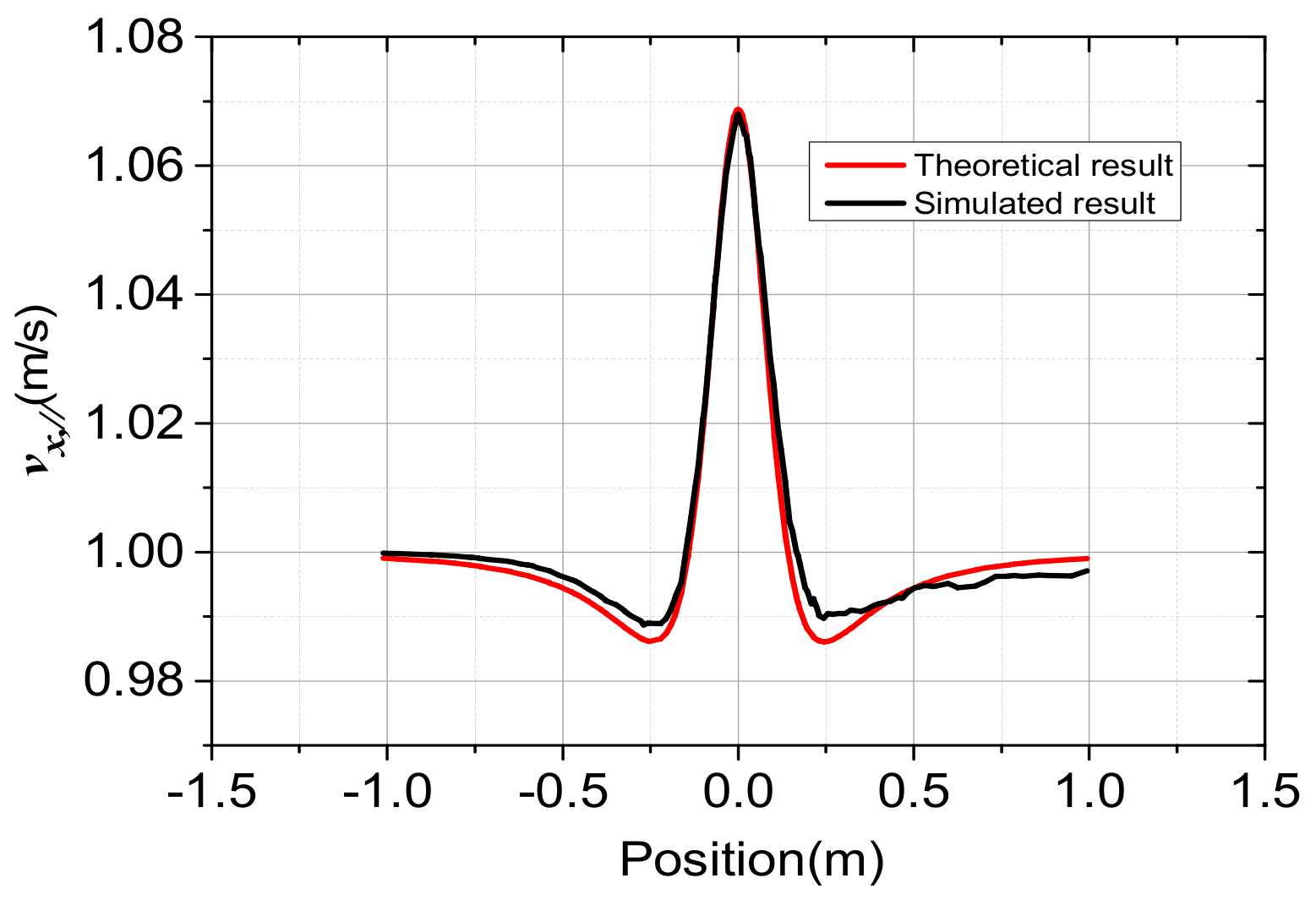
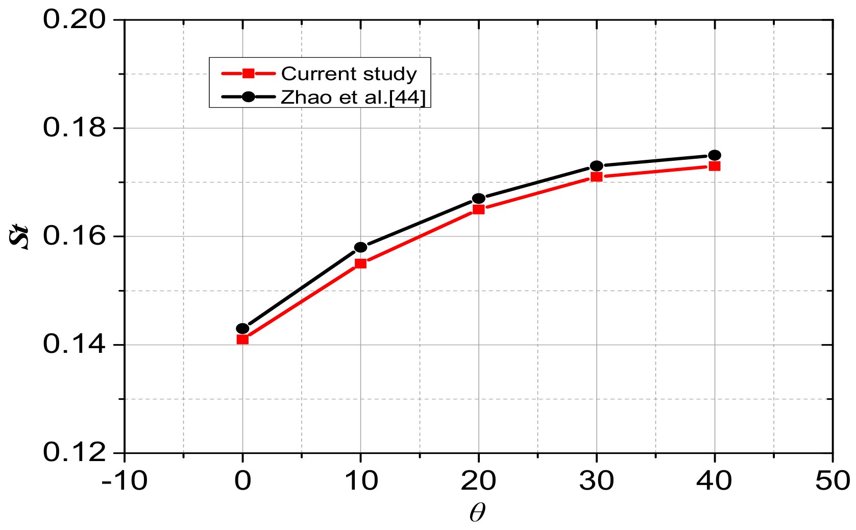
2.3. Numerical Validation

In this section, the accuracy of the numerical algorithm is demonstrated and validated by theoretical and previous results.

In the analysis of theoretical validation, the velocity potential $\varphi$ meets the Laplace equation, as shown in Equation (8). Because of its properties, the complex flow can be decomposed into several simple flows:

$$\frac{{\partial }^2\varphi }{\partial x_i^2}+\frac{{\partial }^2\varphi }{\partial y_i^2}+\frac{{\partial }^2\varphi }{\partial z_i^2}=0,$$

(8)

In uniform flow, the flow field around a sphere can be considered to be a mixed flow of uniform flow and dipole flow. The interest velocity potential $\varphi$ can be expressed as Equation (9), the flow velocity near the target can be shown as Equation (10), and the parallel velocity component $v{\left(x\right)}_{x,//}$ can be expressed as Equation (11) [43]. If we do not consider the influence of gravity and the component along the y-direction, the parallel velocity component $v{\left(x\right)}_{x,//}$ meets the requirements of the potential flow theory. For validation of the proposed method, flow past a single sphere is computed. When the detective distance is equal to $2H$, the parallel velocity on the lateral line is as shown in Figure 2. As seen in Figure 2, it is found that the numerical result shows satisfactory agreement with the theoretical result.

$$\varphi ={\varphi }_1+{\varphi }_2=V{x}_i+\frac{H^3\left(V\cdot r\right)}{2{‖r‖}^3}\cdot \omega$$

(9)

$$v\left(r\right)=V-\frac{H^3\left(3\left(V\cdot r\right)\cdot r-{‖r‖}^{2}V\right)}{2{‖r‖}^5}\cdot \omega$$

(10)

$$v{\left(x\right)}_{x,//}=V-\frac{H^{3}V(2{(x_i-x_o)}^2-D^2)}{2{‖{(x_i-x_o)}^2+D^2‖}^{5/2}}\cdot \omega$$

(11)

where $V$ is the flow velocity, $H$ is the spherical diameter, $r$ is the Euclidean distance between the sensor and the target, $‖\cdot ‖$ represents the vector’s Euclidean norm, and $\omega$ is a dimensionless coefficient, which was 1.143 in this paper.

Moreover, Zhao et al. [44] studied the flow past a single square cylinder. The same case was studied by the above computational algorithm in this paper. The Strouhal number of square targets with different postures $\theta$ was computed. The comparison results are shown in Figure 3, and the numerical results are in accordance with previous reports. The computational algorithm is adequate to solve the flow field around the underwater target, which is confirmed by reasonable agreement between our numerical results and the previous data.

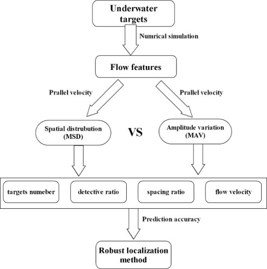
3. Location Strategies

3.1. Method of Spatial Distribution (MSD)

As shown in Figure 2, we determined the parallel velocity distribution on the lateral line. It is clear that there are three extreme points on the curve. Using the operation of partial derivatives on the parallel component, the results are shown in Equation (12), and the abscissa of three extreme points are shown in Equation (13).

$$v{\left(x\right)}_{x,//}^{’}=\frac{3H^{3}V(x_i-x_o)(3D^2-2{(x_i-x_o)}^2)}{2{‖{(x_i-x_o)}^2+D^2‖}^{7/2}}\cdot \omega ,$$

(12)

$$\left\{\begin{array}{l}{x}_1=x_o-\frac{\sqrt{6}}{2}D;\\ x_2=x_o;\\ x_3=x_o+\frac{\sqrt{6}}{2}D\end{array}\right.$$

(13)

As shown in Figure 2, the abscissa of the spherical center and the maximum point are equal, and the spatial variation of two minimum points is $\sqrt{6}D$, where $D$ is equal to $‖y_i-y_o‖$. The results show that the position of a target can be estimated based on the spatial variation of the extremum points. The method is similar to the model presented by Dagamseh et al. [35], which was proven in the study of dipole source localization.

Because the spherical target is symmetrical, in order to discuss it conveniently, the velocity distribution hereinafter is in the XOY plane. As seen in Figure 4, the velocity in the area away from the target is similar to the inlet velocity, resulting in the positions of minimum points being non-obvious. From Figure 5, it is clear that the estimated error ${\epsilon }_1$, which is shown in Equation (14), increases when the detective ratio increases. In other words, as the detective ratio increases, we cannot locate the target based on the MSD accurately. Therefore, the other more robust method is needed.

$${\epsilon }_i=\frac{\left|D-D_{est}\right|}{D}\times 100\%,$$

(14)

where $D$ is the actual detective distance and $D_{est}$ is the estimated detective distance. The $i$ values are 1 and 2, and they represent the estimated errors of the previous method and new method, respectively.

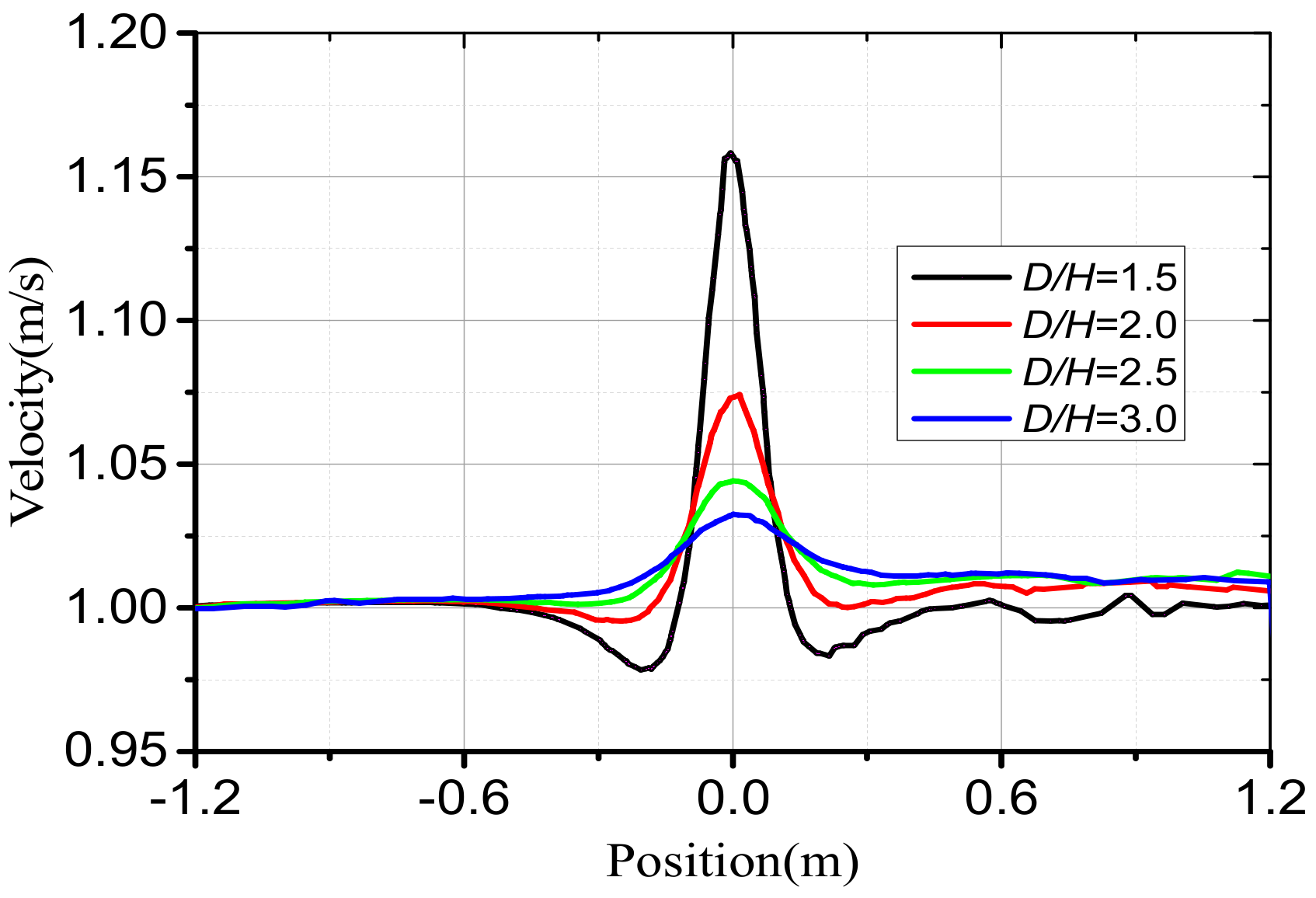
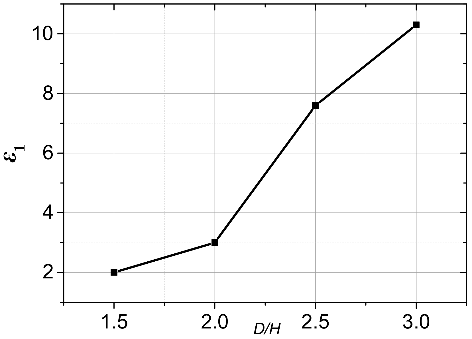
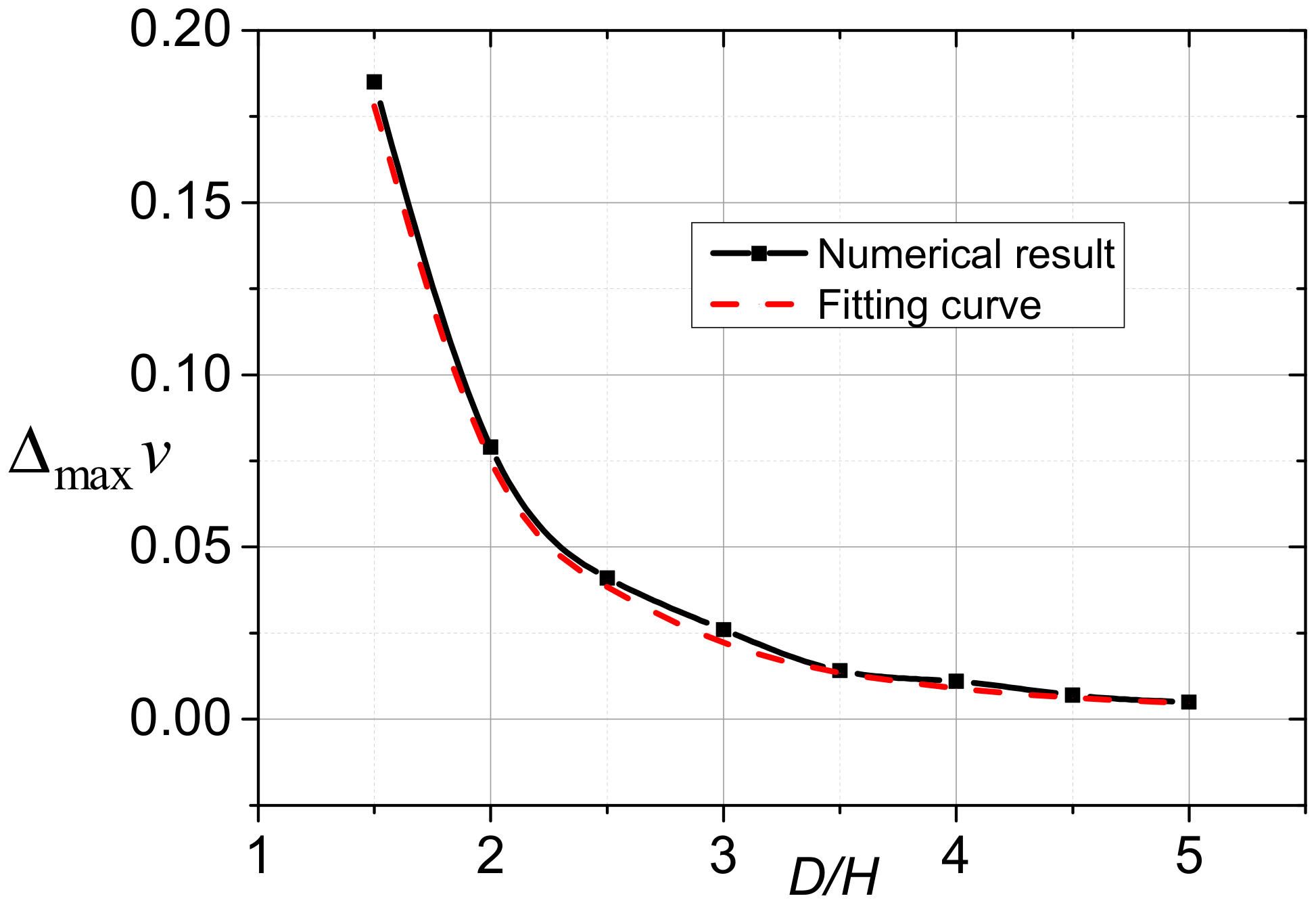
3.2. Method of Amplitude Variation (MAV)

Another interesting observation from Figure 4 is that the amplitude variation of velocity ${\Delta }_{\max }v$ decreases when the detective ratio $D/H$ increases. The amplitude variation ${\Delta }_{\max }v$ is plotted in Figure 6 as a function of the detective ratio. As seen in Figure 6, the connection can be approximated by an exponent regression. The regression equation is shown in Equation (15) and the equation analog effect is good. This implies that the localization of targets can be approximated by the amplitude variation of extreme points in the velocity distribution.

$$\left\{\begin{array}{l}\left|{\Delta }_{\max }v\right|=m/{(D/H)}^n\\ \left|{\Delta }_{\max }v\right|=\left|v_{\max }-v_{\min }\right|\end{array}\right.,$$

(15)

where $m$ and $n$ are the regression coefficients. $v_{\max }$ and $v_{\min }$ are the maximum velocity and the minimum velocity on the lateral line.

According to Equation (11), we can get $v_{\max }$ and $v_{\min }$, which are shown in Equation (16). The amplitude ${\Delta }_{\max }v$ of the velocity drop based on the potential flow theory is shown in Equation (17), whose form is similar to that of Equation (15). Compared with Equation (15), the coefficients $m$ and $n$ are $0.6V$ and 3.0, respectively, in this paper. As seen in Equation (17), the regression coefficients depend on the flow velocity.

$$\left\{\begin{array}{l}{v}_{\max }=V+\frac{V}{2}{(D/H)}^{-3}\cdot \omega \\ v_{\min }=V-\frac{\sqrt{10}V}{125}{(D/H)}^{-3}\cdot \omega \end{array}\right.,$$

(16)

$${\Delta }_{\max }v=\raisebox{1ex}{$\frac{(125+2\sqrt{10)}\cdot \omega \cdot V}{250}$}\!\left/ \!\raisebox{-1ex}{${(D/H)}^3$}\right.$$

(17)

In order to prove that the method is effective at different detective ratios, the velocity curves on more lateral lines were computed, and the detective ratio is estimated based on the MAV, as shown in

Table 2. Estimated detective ratios compared with the actual values.

$\mathit{D}/\mathit{H}$	1.25	1.75	2.25	2.75	3.25
$D_{est}/H$	1.26	1.74	2.23	2.73	3.28
${\epsilon }_2$	0.80	0.63	0.89	0.73	0.92

. We can see that the estimated error of the MAV is less than 1%, and it is smaller than that of MSD obviously. This implies MAV is more robust than MSD.

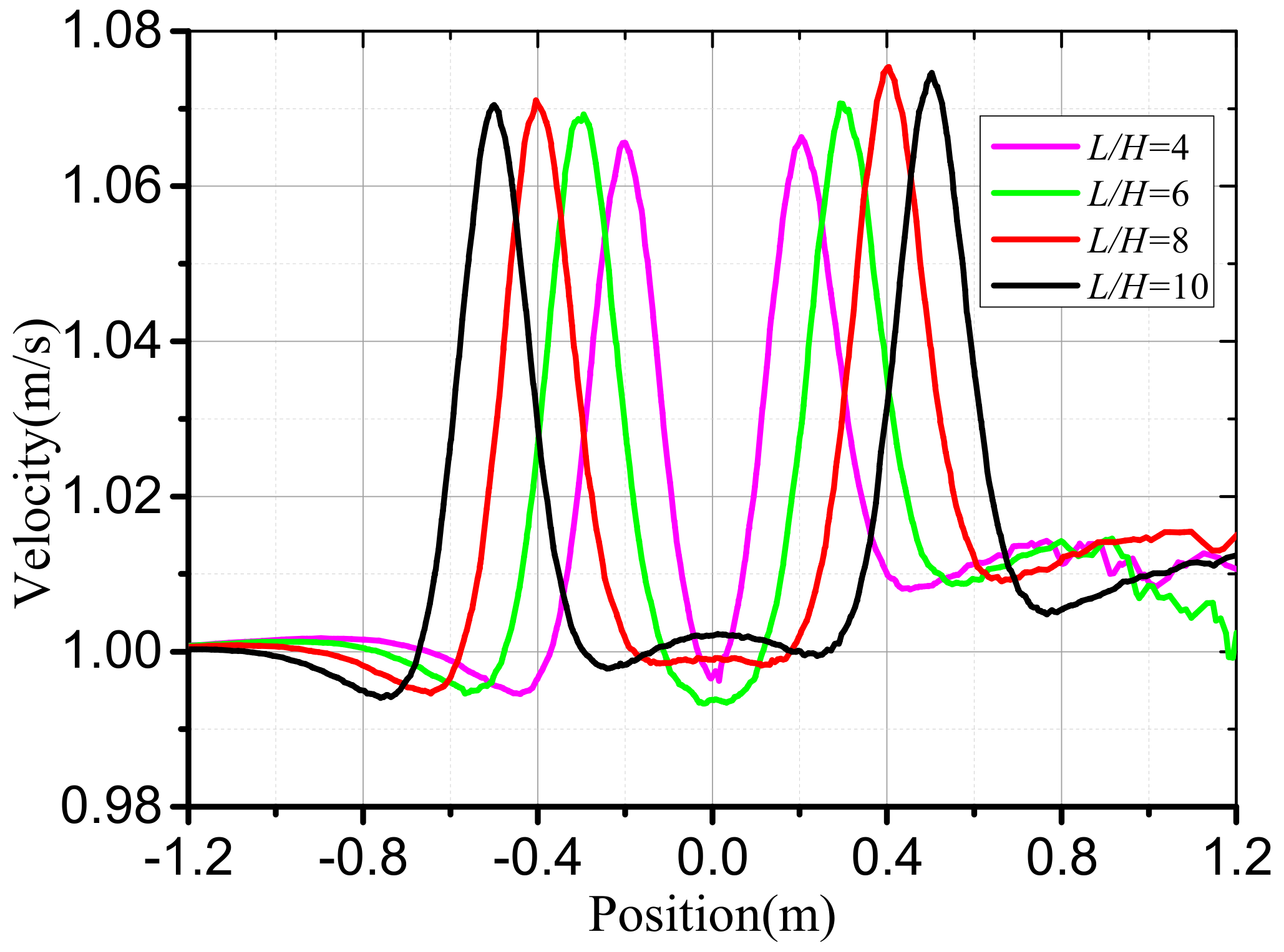
4. Discussion of Tandem Targets

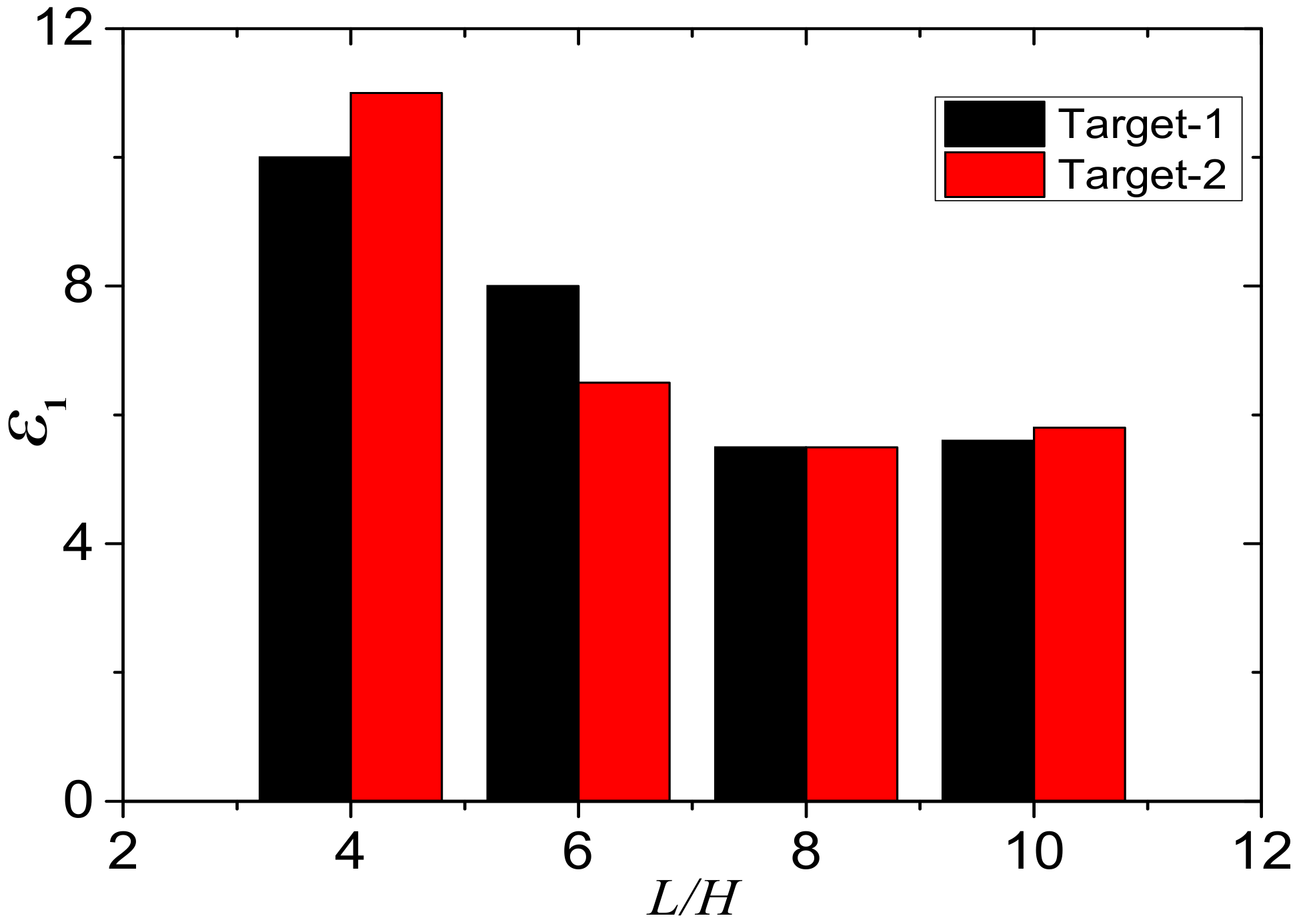
4.1. Influence of the Spacing Ratio

In this section, the case of double targets arrayed in tandem is presented. The influence of the spacing ratio $L/H$ is taken into consideration. It should be pointed out that the amplitude of the velocity curve decreases when the spacing ratio is decreased, as shown in Figure 7. When the spacing ratio becomes bigger, the flow field is more stable. As seen in Figure 7, when the value of $L/H$ is 4 and 6, the positions of two minimum points are not obvious. This implies that the estimated error will become bigger based on the MSD, as shown in Figure 8.

We chose the minimum velocity in the upstream region of the target to calculate the velocity drop amplitude in MAV. Additionally, it is interesting that both the estimated errors are less than 1%. This means that MAV is effective for the case of double targets, and the spacing ratio has no influence on its prediction accuracy.

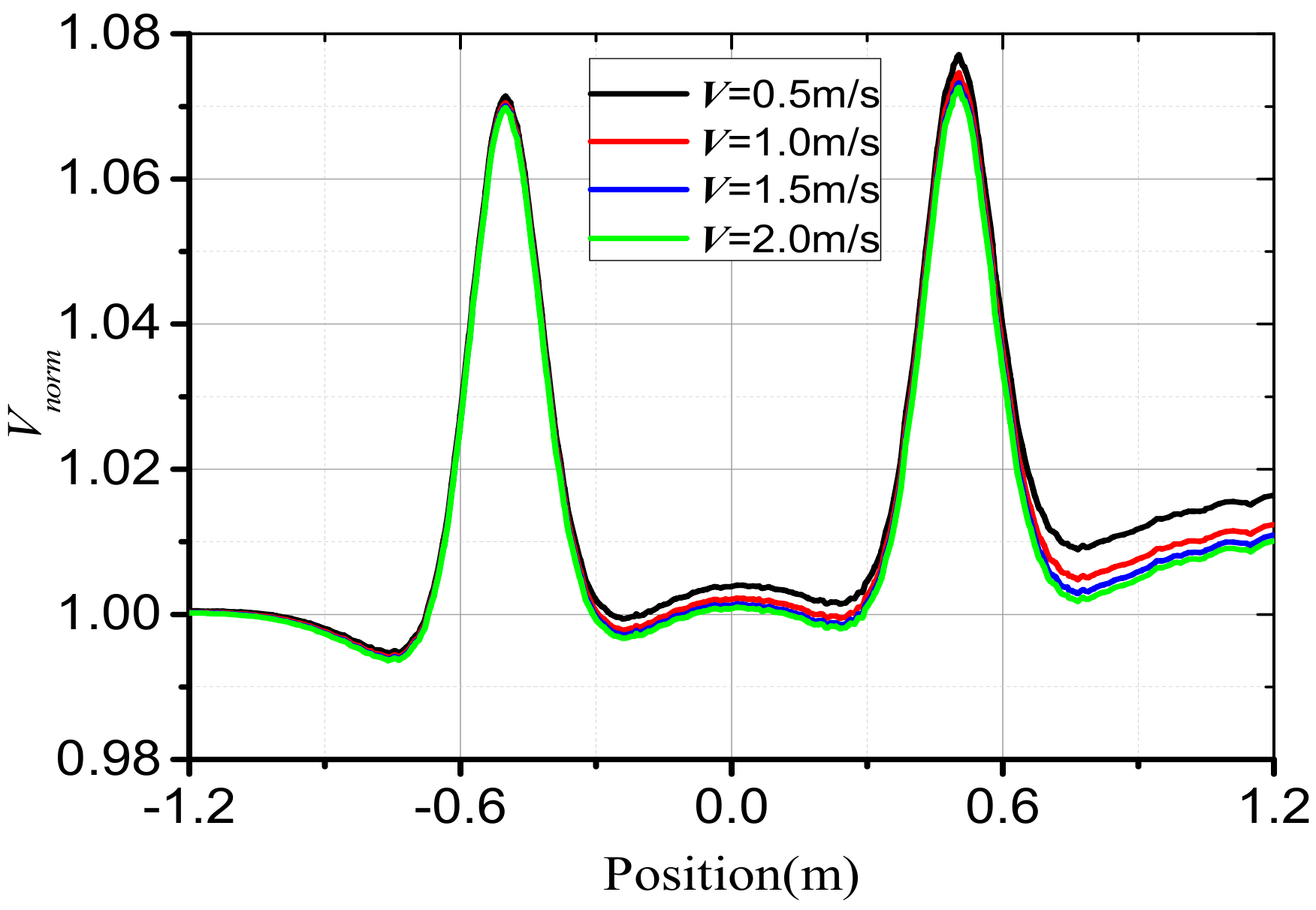
4.2. Influence of the Flow Velocity

In order to determine the influence of the flow velocity on the estimated results, the cases of different flow velocity are computed. Because the velocity range of most AUV is from 0.5 to 2.0 m/s, this range is used for the research considered. For all the cases in this section, the detective ratio and the spacing ratio are set as 2.0 and 10.0, respectively. The parallel velocity curve is treated with the dimensionless method, as shown in Equation (18):

$$V_{norm}=\frac{v}{V},$$

(18)

where $V_{norm}$ is the dimensionless velocity, $v$ is the velocity on the lateral line, and $V$ is the inlet velocity.

As seen in Figure 9, the dimensionless velocity curves are plotted for various flow velocities. In this range, the change of velocity is not sufficient to change the velocity distribution on the lateral line. When the spacing ratio is enlarged to 10.0, the shear layers formulated from the upstream target are stable in the gap between the targets. Therefore, the flow patterns are similar to each other.

It can be seen from Figure 9 that the dimensionless velocity curves are similar to each other in the range of flow velocities. This implies that the flow velocity has little influence on the estimated errors of both methods. The estimated errors of both methods for target-2 are shown in

Table 3. Estimated errors of both methods for target-2.

$\mathit{V}$ (m/s)	0.5	1.0	1.5	2.0
${\epsilon }_1$	5.846	6.495	6.279	6.306
${\epsilon }_2$	0.573	0.746	0.685	0.652

. As seen in Table 3, the estimated errors of MAV with different velocities are smaller.

5. Conclusions

We presented a new strategy for underwater target localization using the flow features including MSD and MAV. The two methods were compared in different cases. The following conclusions were obtained from the results.

• The amplitude variation of extreme points on the parallel velocity curve can be used to estimate the locations of targets. For the cases of flow past one and two targets in a uniform flow field, the estimated error of MAV was less than 1%, which was evidently smaller than that of MSD.
• Changes in the detective ratio and spacing ratio had obvious influences on the estimated error of MSD, but they had little influence on the results of MAV.
• Robust flow sensing is not based on the spatial distribution of the flow field but rather, on the fluctuation range.

Future work will focus on other target shapes and flow patterns, such as irregular targets in turbulent oscillatory and pulsing flows. We hope that this research will investigate the connections among various target shapes and flow patterns and that the full range of practical applications of this new object location strategy will be established.

References

1. Li, J.H.; Kim, M.G.; Kang, H.; Lee, M.J.; Cho, G.R. UUV Simulation Modeling and its Control Method: Simulation and Experimental Studies. J. Mar. Sci. Eng. 2019, 7, 89. [Google Scholar] [CrossRef]
2. Davide, C.; Marco, B.; Gabriele, B.; Massimo, C.; Andrea, R.; Enrica, Z.; Lucia, M.; Paola, C. A Novel Gesture-Based Language for Underwater Human-Robot Interaction. J. Mar. Sci. Eng. 2018, 6, 91. [Google Scholar]
3. Corina, B.; Matthew, W.; Dunnigan, M.; Petillot, P. Coupled and Decoupled Force/Motion Controllers for an Underwater Vehicle-Manipulator System. J. Mar. Sci. Eng. 2018, 6, 96. [Google Scholar]
4. Szyrowski, T.; Khan, A.; Pemberton, R.; Sharma, S.K.; Singh, Y.; Polvara, R. Range Extension for Electromagnetic Detection of Subsea Power and Telecommunication Cables. J. Mar. Sci. Eng. Technol. 2019, 1–8. [Google Scholar] [CrossRef]
5. Emberton, S.; Chittka, L.; Cavallaro, A. Underwater Image and Video Dehazing with Pure Haze Region Segmentation. Comput. Vis. Image Underst. 2017, 168, 145–156. [Google Scholar] [CrossRef]
6. Li, C.; Guo, J. Underwater Image Enhancement by Dehazing and Color Correction. J. Electron. Imaging 2015, 24, 033023. [Google Scholar] [CrossRef]
7. Zhang, J.X. Principle of Biomimetic Detection Based on Flow Field Information of Underwater Moving Object. Master’s Thesis, Beijing Institute of Technology, Beijing, China, 2015. [Google Scholar]
8. Muhammad, N.; Toming, G.; Tuhtan, J.A.; Musall, M.; Kruusmaa, M. Underwater Map-based Localization Using Flow Features. Auton. Robot. 2017, 41, 417–436. [Google Scholar] [CrossRef]
9. Zheng, R.; Kamran, M. A Model of the Lateral Line of Fish for Vortex Sensing. Bioinspir. Biomim. 2012, 7, 036016. [Google Scholar]
10. Coombs, S.; Patton, P. Lateral Line Stimulation Patterns and Prey Orienting Behavior in the Lake Michigan Mottled Sculpin (Cottus bairdi). J. Comput. Physiol. A 2009, 195, 279–297. [Google Scholar] [CrossRef]
11. Mchenry, M.J.; Feitl, K.E.; Strother, J.A.; Trump, W.J.V. Larval Zebrafish Rapidly Sense the Water Flow of a Predator’s Strike. Biol. Lett. 2009, 5, 477–479. [Google Scholar] [CrossRef]
12. Quinzio, S.; Fabrezi, M. The Lateral Line System in Anuran Tadpoles: Neuromast Morphology, Arrangement, and Innervation. Anat. Rec. 2014, 297, 1508–1522. [Google Scholar] [CrossRef] [PubMed]
13. Schaumburg, F.; Kler, P.A.; Berli, C.L.A. Numerical Prototyping of Lateral Flow Biosensors. Sens. Actuators B Chem. 2018, 259, 1099–1107. [Google Scholar] [CrossRef]
14. Tuhtan, J.A.; Fuentes-Pérez, J.F.; Strokina, N.; Toming, G.; Musall, M.; Noack, M.; Kruusmaa, M. Design and Application of a Fish-shaped Lateral Line Probe for Flow Measurement. Rev. Sci. Instrum. 2016, 87, 045110. [Google Scholar] [CrossRef] [PubMed]
15. Dusek, J.E.; Triantafyllou, M.S.; Lang, J.H. Piezoresistive Foam Sensor Arrays for Marine Applications. Sens. Actuators A Phys. 2016, 248, 173–183. [Google Scholar] [CrossRef]
16. Delamare, J.; Sanders, R.G.P.; Krijnen, G.J.M. 3D Printed Biomimetic Whisker-based Sensor with Co-planar Capacitive Sensing. In Proceedings of the 2016 IEEE International Conference on Sensors, Orlando, FL, USA, 30 October–3 November 2016. [Google Scholar]
17. Zhu, P.; Ma, B.; Jiang, C.; Deng, J.; Wang, Y. Improved Sensitivity of Micro Thermal Sensor for Underwater Wall Shear Stress Measurement. Microsyst. Technol. 2015, 21, 785–789. [Google Scholar] [CrossRef]
18. Djapic, V.; Dong, W.J.; Bulsara, A.; Anderson, G. Challenges in Underwater Navigation: Exploring Magnetic Sensors Anomaly Sensing and Navigation. In Proceedings of the 2016 IEEE International Conference on Sensors Applications Symposium, Zadar, Croatia, 13–15 April 2015. [Google Scholar]
19. Salmanpour, M.S.; Sharif, K.Z.; Aliabadi, M. Impact Damage Localisation with Piezoelectric Sensors under Operational and Environmental Conditions. Sensors 2017, 17, E1178. [Google Scholar] [CrossRef]
20. Campos, R.; Gracias, N.; Ridao, P. Underwater Multi-vehicle Trajectory Alignment and Mapping Using Acoustic and Optical Constraints. Sensors 2016, 16, 387. [Google Scholar] [CrossRef]
21. Mou, B.; He, B.J.; Zhao, D.X.; Chau, K.W. Numerical Simulation of the Effects of Building Dimensional Variation on Wind Pressure Distribution. Eng. Appl. Comput. Fluid 2019, 11, 293–309. [Google Scholar] [CrossRef]
22. Ghalandari, M.; Koohshahi, E.M.; Mohamadian, F.; Shamshirband, S.; Chau, K.W. Numerical Simulation of Nanofluid Flow inside a Root Canal. Eng. Appl. Comput. Fluid 2019, 13, 254–264. [Google Scholar] [CrossRef]
23. Jorge, P.; Beatriz, D.P.; Jesús, F.O.; Eduardo, B.M. A CFD Study on the Fluctuating Flow Field across a Parallel Triangular Array with One Tube Oscillating Transversely. J. Fluid Struct. 2018, 76, 411–430. [Google Scholar]
24. Manoochehr, F.M.; Mohammad, T.S.; Mostafa, R. Numerical Simulation of the Hydraulic Performance of Triangular and Trapezoidal Gabion Weirs in Free Flow Condition. Flow Meas. Instrum. 2018, 62, 93–104. [Google Scholar]
25. Hassan, E.S. Mathematical Description of the Stimuli to the Lateral Line System of Fish Derived from a Three-dimensional Flow Field Analysis. Biol. Cybern. 1992, 6, 443–452. [Google Scholar] [CrossRef]
26. Humphrey, J.A. Drag Force Acting on a Neuromast in the Fish Lateral Line Trunk Canal II: Analytical Modelling of Parameter Dependencies. J. R. Soc. Interface 2009, 6, 641–653. [Google Scholar] [CrossRef] [PubMed]
27. Kumar, P.S.; Vendhan, C.P.; Krishnankutty, P. Study of Water Wave Diffraction around Cylinders Using a Finite-element Model of Fully Nonlinear Potential Flow Theory. Ships Offsh. Struct. 2017, 12, 276–289. [Google Scholar] [CrossRef]
28. Zhang, J.X.; Fan, X.; Liang, D.F.; Liu, H. Numerical Investigation of Nonlinear Wave Passing through Finite Circular Array of Slender Cylinders. Eng. Appl. Comput. Fluid 2019, 13, 102–116. [Google Scholar] [CrossRef]
29. Song, X.W.; Qi, Y.C.; Zhang, M.X.; Zhang, G.G.; Zhan, W.C. Application and Optimization of Drag Reduction Characteristics on the Flow around a Partial Grooved Cylinder by Using the Response Surface Method. Eng. Appl. Comput. Fluid 2019, 13, 158–176. [Google Scholar] [CrossRef]
30. Quezada, M.; Tamburrino, A.; Nino, Y. Numerical Simulation of Scour around Circular Piles Due to Unsteady Currents and Oscillatory Flows. Eng. Appl. Comput. Fluid 2018, 12, 354–374. [Google Scholar] [CrossRef]
31. Barbier, C.; Humphrey, J.A.C. Drag Force Acting on a Neuromast in the Fish Lateral Line Trunk Canal. I. Numerical Modelling of External–Internal Flow Coupling. J. R. Soc. Interface 2009, 6, 627–640. [Google Scholar] [CrossRef]
32. Zhou, H.; Hu, T.J.; Low, K.H.; Shen, L.C.; Ma, Z.W.; Wang, G.M.; Xu, H.J. Bio-inspired Flow Sensing and Prediction for Fish-like Undulating Locomotion: A CFD-aided Approach. J. Bionic Eng. 2015, 12, 406–417. [Google Scholar] [CrossRef]
33. Singh, Y.; Bhattacharyya, S.K.; Idichandy, V.G. CFD Approach to Modelling, Hydrodynamic Analysis and Motion Characteristics of a Laboratory Underwater Glider with Experimental Results. J. Ocean Eng. Sci. 2017, 2, 90–119. [Google Scholar] [CrossRef]
34. Tao, J.; Yu, X. Hair Flow Sensors: From Bio-inspiration to Bio-mimicking a Review. Smart Mater. Struct. 2012, 21, 113001. [Google Scholar] [CrossRef]
35. Abdulsadda, A.T.; Tan, X. Nonlinear Estimation-based Dipole Source Localization for Artificial Lateral Line Systems. Bioinspir. Biomim. 2013, 8, 026005. [Google Scholar] [CrossRef] [PubMed]
36. Abdulsadda, A.T.; Tan, X. An Artificial Lateral Line System Using IPMC Sensor Arrays. Int. J. Smart Nano Mater. 2012, 3, 226–242. [Google Scholar] [CrossRef]
37. Dagamseh, A.M.K.; Lammerink, T.S.J.; Kolster, M.L.; Bruinink, C.M.; Wiegerink, R.J.; Krijnen, G.J.M. Dipole-source Localization Using Biomimetic Flow-sensor Arrays Positioned as Lateral-line System. Sens. Actuators A Phys. 2010, 162, 355–360. [Google Scholar] [CrossRef]
38. Salumae, T.; Kruusmaa, M. Flow-relative Control of an Underwater Robot. Proc. R. Soc. A Math Phys. 2013, 469, 1–19. [Google Scholar] [CrossRef]
39. Venturelli, R.; Akanyeti, O.; Visentin, F.; Jezov, J.; Chambers, L.; Toming, G.; Brown, J.; Kruusmaa, M.; Megill, W.M.; Fiorini, P. Hydrodynamic Pressure Sensing with an Artificial Lateral Line in Steady and Unsteady Flows. Bioinsper. Biomim. 2012, 7, 036004. [Google Scholar] [CrossRef]
40. Fuentes-Perez, J.F.; Uhtan, J.A.; Baeza, R.C.; Musall, M.; Toming, G.; Muhammad, N. Current Velocity Estimation Using a Lateral Line Probe. Ecol. Eng. 2015, 85, 296–300. [Google Scholar] [CrossRef]
41. Yang, Y.; Nguyen, N.; Chen, N.; Lockwood, M.; Tucker, C.; Hu, H.; Jones, D. Artificial Lateral Line with Biomimetic Neuromasts to Emulate Fish Sensing. Bioinspir. Biomim. 2010, 5, 16001. [Google Scholar] [CrossRef] [Green Version]
42. Bao, Y.; Zhou, D.; Zhao, Y.J. A Two Step Taylor-characteristic-based Galerkin Method for Incompressible Flows and Its Application to Flow over Triangular Cylinder with Different Incidence Angles. Int. J. Numer. Methods Fluids 2010, 62, 1181–1208. [Google Scholar] [CrossRef]
43. Lamb, H. Hydrodynamics; Cambridge University Press: Cambridge, UK, 1932. [Google Scholar]
44. Zhao, X.Z.; Cheng, D.; Zhang, D.K.; Hu, Z.J. Numerical Study of Low-Reynolds-number Flow Past Two Tandem Square Cylinders with Varying Incident Angles of the Downstream One Using a CIP-based Model. Ocean Eng. 2016, 121, 414–421. [Google Scholar] [CrossRef]
Figure 1. Schematic diagram of the computational domain in the XOY plane.
Jmse 07 00437 g001
Figure 2. Comparison of the simulated parallel velocity and the theoretical result.
Jmse 07 00437 g002
Figure 3. Comparison of simulated results and previous results.
Jmse 07 00437 g003
Figure 4. Parallel velocity on the lateral line at different detective ratios.
Jmse 07 00437 g004
Figure 5. Estimated error at different detective ratios.
Jmse 07 00437 g005
Figure 6. Velocity drop amplitude at different detective ratios and the fitting cure.
Jmse 07 00437 g006
Figure 7. Parallel velocity on the lateral line at different spacing ratios.
Jmse 07 00437 g007
Figure 8. Parallel velocity on the lateral line at different spacing ratios.
Jmse 07 00437 g008
Figure 9. Dimensionless velocity curves on the lateral lines with different inlet velocities.
Jmse 07 00437 g009