Probabilistic Assessment of Overtopping of Sea Dikes with Foreshores including Infragravity Waves and Morphological Changes: Westkapelle Case Study

Abstract

Shallow foreshores in front of coastal dikes can reduce the probability of dike failure due to wave overtopping. A probabilistic model framework is presented, which is capable of including complex hydrodynamics like infragravity waves, and morphological changes of a sandy foreshore during severe storms in the calculations of the probability of dike failure due to wave overtopping. The method is applied to a test case based on the Westkapelle sea defence in The Netherlands, a hybrid defence consisting of a dike with a sandy foreshore. The model framework consists of the process-based hydrological and morphological model XBeach, probabilistic overtopping equations (EurOtop) and the level III fully probabilistic method ADIS. By using the fully probabilistic level III method ADIS, the number of simulations necessary is greatly reduced, which allows for the use of more advanced and detailed hydro- and morphodynamic models. The framework is able to compute the probability of failure with up to 15 stochastic variables and is able to describe feasible physical processes. Furthermore, the framework is completely modular, which means that any model or equation can be plugged into the framework, whenever updated models with improved representation of the physics or increases in computational power become available. The model framework as described in this paper, includes more physical processes and stochastic variables in the determination of the probability of dike failure due to wave overtopping, compared to the currently used methods in The Netherlands. For the here considered case, the complex hydrodynamics like infragravity waves and wave set-up need to be included in the calculations, because they appeared to have a large influence on the probability of failure. Morphological changes of the foreshore during a severe storm appeared to have less influence on the probability of failure for this case. It is recommended to apply the framework to other cases as well, to determine if the effects of complex hydrodynamics as infragravity waves and morphological changes on the probability of sea dike failure due to wave overtopping as found in this paper hold for other cases as well. Furthermore, it is recommended to investigate broader use of the method, e.g., for safety assessment, reliability analysis and design.

1. Introduction

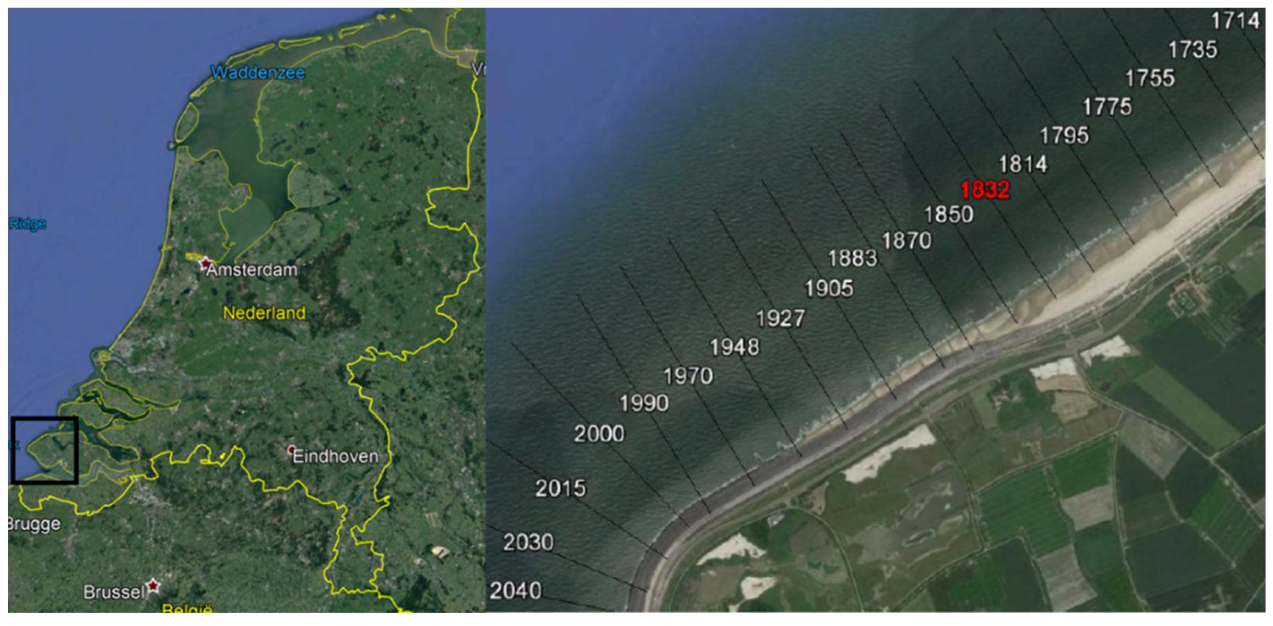
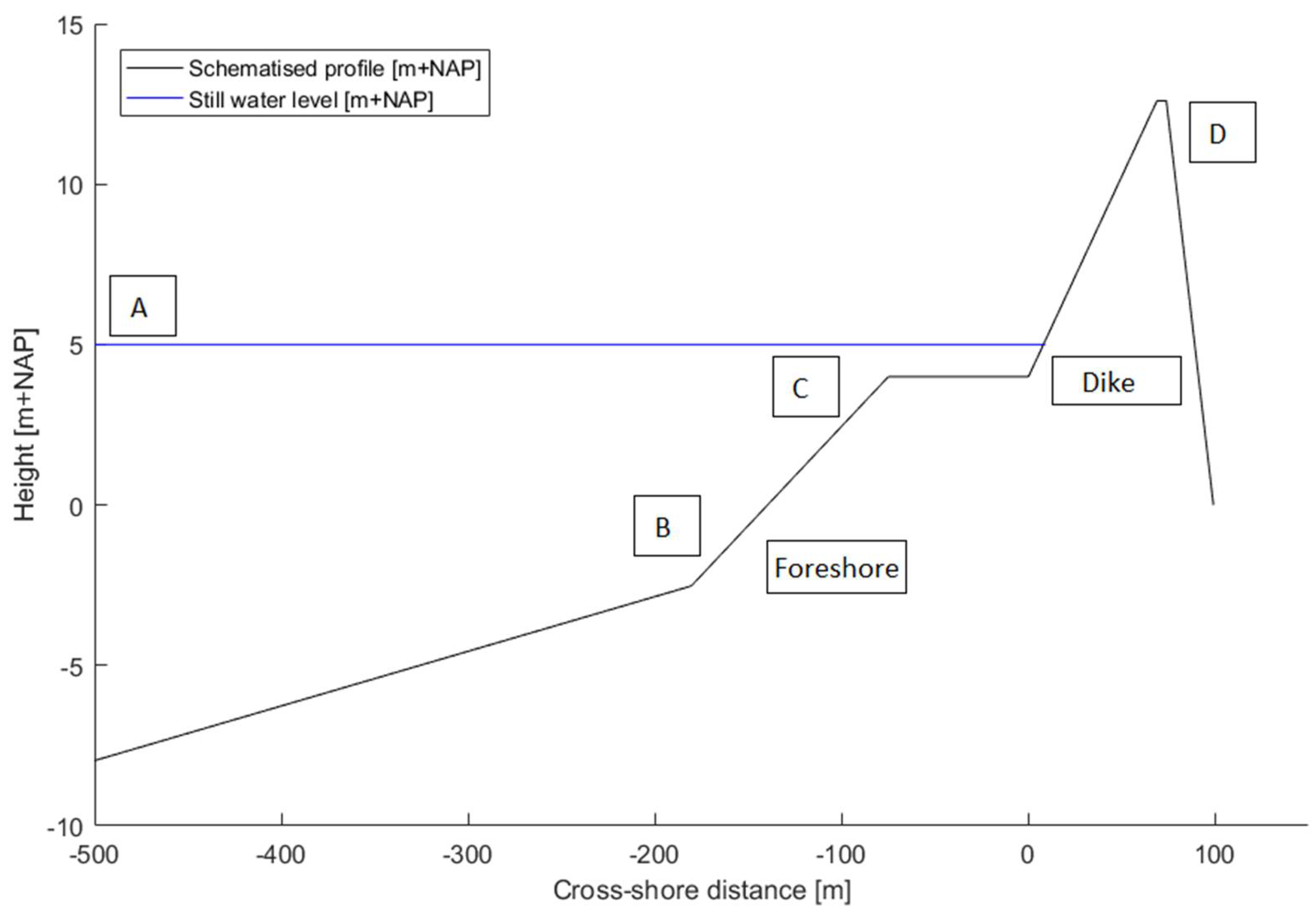
In recent years, Building with Nature solutions (soft solutions, such as sand nourishments) are increasingly considered as an alternative in flood protection, see e.g., Van Slobbe et al. [1]. These soft solutions are considered as a supplement to the usual hard measures (dikes, coastal structures). Three types of soft defences can be distinguished [2]. Here, one of these types is considered: a hybrid defence, more specifically a dike with a shallow sandy foreshore. This dike-foreshore system is a combination of a traditional dike and a nourished foreshore, consisting of a body of sand, possibly covered with vegetation. The foreshore reduces the loads on the dike. The dike remains part of the defence. A hybrid defence really is a combination in which both parts are of importance in the flood protection. Constructing a sandy foreshore in front of a dike can be a method to decrease the failure probability. However, the uncertainty in the morphological development of these foreshores leads to uncertainty with respect to their contribution in protection against flooding. The morphological stability of a foreshore during extreme conditions is not well-known. Furthermore, the influence of infragravity waves generated on the foreshore on the wave overtopping and failure probability is largely unknown. Increasing interest in soft solutions of dike managers, as well as local inhabitants (getting a nice beach), makes it interesting to investigate the contribution of foreshores to flood protection further.

The risk management and optimization of coastal structures have gained much attention the last years. In order to optimize a design, the uncertainties need to be taken into account as detailed as possible, by using probabilistic approaches. However, currently these approaches are often deterministic or semi-probabilistic. For example, the currently used methods in the Netherlands to determine the probability of dike failure due to wave overtopping only include a few stochastic variables and use a model to determine the wave hydrodynamics that does not include infragravity waves or morphological changes. By using a full-probabilistic approach, the risks could potentially be further reduced and the designs further optimized, see e.g., Wainwright et al. [3].

During a storm, several processes occur at a dike-foreshore system. Wave energy is dissipated on the foreshore by wave breaking, which causes a shift in the wave spectrum from the peak frequency to the lower frequencies due to the generation of infragravity waves, see e.g., Symonds et al.; Longuet-Higgins & Stewart [4,5]. The breaking waves also lead to erosion of the foreshore. Finally, if water levels and wave heights are large enough, wave overtopping may occur over the dike. Hence, the generation of infragravity waves, morphological changes of the foreshore and wave overtopping are important aspects in the design of dike-foreshore systems.

Infragravity waves are generated by groups of wind induced waves, and are sometimes called long waves or surfbeat in the surf zone. Infragravity waves are known to be important on dissipative beaches and for run-up [5]. Typical infragravity wave periods range from 25–30 s to 250–300 s [6]. As previous studies on dike-foreshore systems [4,7] indicated that wave energy dissipation causes a shift in the wave spectrum from the peak frequency to the lower frequencies (due to generation of infragravity waves), instead of the wave peak period, the T_m−1,0 wave period was recommended as a measure in these situations to calculate the wave run-up or wave overtopping [8,9,10]. This period is defined as T_m−1,0 = m₋₁/m₀, with m_k being the kth moment of the wave spectrum. The period is commonly used in coastal structure design [11], and the use of the T_m−1,0 wave period is incorporated in manuals like the EurOtop manual [12]. Furthermore, it was found, that on high foreshores where intense breaking occurs, the wave set-up becomes important for the wave run-up and overtopping as well [13].

Roeber & Bricker [14] showed that during Typhoon Haiyan, at the town of Hernani, the Philippines, an infragravity wave steepened into a tsunami-like wave that caused excessive damage and casualties. The fringing reef present near the town protected the community from moderate storms, but increased flooding during this extreme event. Typical for these reef environments is a very short wave-breaking zone over a steep reef face, which releases the bound infragravity waves with little energy loss. This indicates that it can be important to include the infragravity waves in the design of dike-foreshore systems.

For this paper, the failure mechanism wave overtopping was chosen, because it is one of the most important failure modes of dike-foreshore systems. The overtopping discharge depends on the wave conditions at the toe, slope geometry, and the existing freeboard. The most commonly used equations to describe wave overtopping are the ones from EurOtop [12].

Suzuki et al. [7] concluded that beach nourishments do not always reduce the wave overtopping discharge, due to set-up and generation of bores and infragravity waves. Van Gent & Giarrusso [15] found that for foreshores characterized by a bar, trough and terrace in front of a dike, the contribution of low frequency energy to the total wave energy could reach 30%. It has to be noted that most of the previous studies did not include the wave directional spreading, because they were based on physical flume model tests. However, the wave directional spreading can have a large influence on the generation of infragravity waves and the wave period [11].

Bakker & Vrijling; Madsen et al. [16,17] give extensive descriptions of many of the different available probabilistic calculation methods. The Joint Committee on Structural Safety [18] proposed a level-classification of probabilistic calculation methods for the reliability of an element (now ISO 2394:2015). Here, level I methods do not calculate failure probabilities, but use partial safety factors. Level II methods linearize the limit state function in the design point and approximate the probability distribution of each variable by a standard normal distribution. Level III methods or fully probabilistic methods calculate the probability of failure by considering the probability density functions of all variables.

Previous research considering probabilistic methods was often focused on different processes and failure mechanisms than wave overtopping (e.g., [19,20,21,22]). Furthermore, the previous research mostly considered only a few stochastic variables, with simple 1D empirical or numerical models and probabilistic methods like Monte Carlo Simulation, which require a large number of simulations (e.g., [19,20,21,22,23]).

Overall, probabilistic methods have been applied to coastal dikes and dunes, but not yet to the issues studied in this paper. Hence, a method which includes the influence of complex hydrodynamics such as infragravity waves, and morphological changes of a sandy foreshore on the probability of dike failure due to wave overtopping does not yet exist. Therefore, the main goal of this paper is to develop a framework to calculate the probability of sea dike failure due to wave overtopping, taking into account the morphological changes of the foreshore and complex hydrodynamics like infragravity waves. Furthermore, the goal is to determine the influence of using a process-based model with complex hydrodynamics versus using a calculation rule, and to determine the influence of morphological changes of the foreshore on the probability of failure due to wave overtopping for the here considered case.

First, the case study location is described (Section 2.1), then the choice and validation of the model framework are discussed (Section 2.2). Next, the input of the probabilistic calculations is briefly described (Section 2.3). After that, the results are given (Section 3), followed by a discussion (Section 4). The paper ends with several conclusions (Section 5).

2. Materials and Methods

2.1. Case Study Description

The configuration that is considered in this paper is roughly based on the hybrid sea defence at Westkapelle, on the coast of Walcheren in The Netherlands, see Figure 1. The measured bathymetrical transect 1832 from 2009 is shown in Figure 2. The average crest height of this dike is 12.6 m+NAP (Normaal Amsterdams Peil, Dutch ordnance level). This means that it is a very large dike, as extreme surge levels considered are around 5 m+NAP [24], and therefore the crest freeboard under design conditions is still more than 7 m. The average slope is around 1:8, and the revetment of the outer slope consists of asphalt above a berm and rubble stone penetrated with mastic asphalt below this berm. The berm is located around 7.5 m+NAP. In 2002, research indicated that (e.g., due to climate change) the design conditions should be increased [25]. The expected wave overtopping discharge during the new design conditions exceeded the acceptable level of 0.1 ls⁻¹m⁻¹ (return period of 1:4000 years). As the landward slope of the dike consists of bare sand, a larger discharge than 0.1 ls⁻¹m⁻¹ could not be accepted [12]. In 2008, it was decided to strengthen the dike with a foreshore with a volume of 2.5 million cubic meter of sand in front of the dike. The initial height and width of the foreshore were approximately 4 m+NAP and 75 m respectively, with an average foreshore slope of approximately 1:17. During normal conditions, this gives a dry beach in front of the dike.

The profile used in the calculations is loosely based on the 2009 bathymetric survey transect 1832 at the Westkapelle sea defence, see Figure 2. Instead of the local crest height at transect 1832, the mean crest height of the Westkapelle sea defence is used, being 12.6 m+NAP. Furthermore, the bathymetry is simplified to two line sections based on the average slope (a horizontal beach and a foreshore slope), to be able to easily compare a situation without and with a foreshore. This simplification of the profile means that the volume of sand might not be completely equal to the actual foreshore at Westkapelle. A schematization of the Westkapelle sea defence is justified for this study, because the goal of the paper is to determine a framework which can include the influence of the complex hydrodynamics and cross-shore morphological changes during severe storms on the probability of failure.

2.2. Set-Up and Validation of Model Framework

The set-up of the framework is explained in more detail in this subsection. Because a single model that includes all the different relevant processes does not exist, a model framework is developed, in which different models are combined. In this study we use a combination of XBeach in surfbeat mode, to cope with the morphodynamic and hydraulic behavior, the EurOtop formulae on wave overtopping, and the probabilistic method Adaptive Directional Importance Sampling (ADIS). It combines accuracy in the modelling of processes with computational efficiency. The morphological changes that are considered here are the dominant short term storm morphological changes. The present paper builds on the work of Den Bieman et al. [21], who first combined ADIS and XBeach, to perform a dune erosion safety assessment.

2.2.1. Hydro- and Morphodynamics: XBeach and h/2-Assumption

XBeach is chosen to model the hydrodynamics and morphological changes. In surfbeat mode, XBeach can include the short wave height transformation, the wave set-up, the infragravity wave transformation and the morphological changes. It is mainly chosen for its inclusion of the infragravity waves and morphological changes, and its proven skill. XBeach is a nearshore numerical model used to assess the coastal response during storm conditions, and has been extensively calibrated and validated [26,27] (also refer to www.xbeach.org). XBeach is a coupled phase-averaged spectral wave model for sea swell and non-linear shallow water model for infragravity waves. It combines stochastic and deterministic approaches. XBeach solves the phase-averaged wave action equation. XBeach uses a form of the dissipation formula for wave breaking according to Roelvink [28] and a roller energy balance, which is coupled to the wave action balance, by Reniers et al. [29]. For the low frequency and mean flows, the shallow water equations are used. XBeach models sediment transport by a depth-averaged advection diffusion equation by Galappatti & Vreugdenhil [30]. The equilibrium sediment concentration is calculated by the sediment transport formula of Soulsby & Van Rijn [31].

A commonly used rule of thumb for gentle foreshore slopes is the simple h/2-assumption, where the wave height H_m0 is half the water depth h. The assumption does not include the complex hydrodynamics such as infragravity waves or wave set-up, nor does it include morphological changes. Also, changes in wave period are not calculated by the model. The h/2-assumption was compared with XBeach 1D without the infragravity wave forcing for several situations. The models showed good agreement. The h/2-assumption calculation rule is used in this paper, to compare to the results of XBeach surfbeat, which does include both the complex hydrodynamics like infragravity waves, and morphological changes of the foreshore.

Even though XBeach has already been extensively validated, an additional validation was performed specifically for the case considered here, in Oosterlo [32]. The XBeach hydrodynamics were validated for this study by using the flume experiments of Van Gent [9] on which the EurOtop wave overtopping formula for ξ_m−1,0 > 7 was based. XBeach showed good skill in predicting the H_m0 and T_m−1,0. For a more detailed description of the validation, refer to Oosterlo [32].

In the modelling framework, the incoming waves are separated from the total wave signal as computed by XBeach by the method of Guza et al. [33]. For each hour of storm data, during which the boundary conditions are regarded as being constant, the wave spectra are calculated. From these spectra the wave height (H_m0) and wave period (T_m−1,0) at the dike toe are determined, which are used as input for the overtopping calculations.

2.2.2. Wave Overtopping: EurOtop

Because XBeach cannot be used to calculate small overtopping discharges as the ones considered in this paper [34], the EurOtop (first edition) formulae [35] are chosen to model the wave overtopping discharge, because they are the most commonly and extensively used wave overtopping formulae, and because they form a set of equations that can be used for all types of wave breaking conditions and slopes. The EurOtop [35] equations were based on a large set of measured data from different model tests in small and large scale as well as in wave flumes and wave basins. Furthermore, the EurOtop [35] formulae are the only formulae that include the infragravity waves in any way, by using the T_m−1,0 wave period. In the recent 2016 second edition [12], some equations have been updated. For sloping structures, where the freeboard is at least half the wave height, the differences between the first edition EurOtop [35] formulae and the new ones is quite small. For that reason one may also continue to use the first edition EurOtop [35] formulae in such a situation [12]. Because the previous is always the case for the situations considered in this paper, the equations of the first edition of EurOtop [35] are still used here. A brief description of the used EurOtop [35] equations is given in Appendix A.

In the modelling framework, the resulting wave parameters at the toe of the dike are entered into the EurOtop [35] equations, together with the freeboard, main wave direction, slope of the dike (average slope = 1:8) and roughness of the slope (for asphalt γ_f = 1.0 [12]), with which the wave overtopping discharge is calculated for each hour of the storm. The wave overtopping discharges during the storm are then compared and the largest one is used further in the ADIS calculation of the limit state function (see next subsubsection).

2.2.3. Probabilistic Calculation Method: Adaptive Directional Importance Sampling

Using limit states, it is possible to define a reliability function or limit state function. The general form of a limit state function is, e.g., Madsen et al. [17]):

$$Z=R-S$$

(1)

in which R indicates the strength parameters and S the load parameters. In the limit state, the limit state function Z is equal to 0. Failure occurs if Z ≤ 0. The goal of the probabilistic calculations is to find the probability of failure and the corresponding design point. The design point is the point on the limit state function (Z = 0) with the largest probability density [17].

Adaptive Directional Importance Sampling (ADIS), a level III or fully probabilistic method, is chosen as the probabilistic calculation method, because ADIS can be used for small probabilities of failure, medium numbers of random variables, non-normal distributed variables, non-linear limit state functions, discontinuously shaped failure spaces, statistically dependent and independent stochastic variables and limit state functions, and multiple limit state functions [36]. But, most importantly, ADIS greatly reduces the number of calculations necessary, with respect to crude Monte Carlo Simulation. This means that more stochastic variables, more complex limit state functions and more detailed (hydrodynamic and morphological) models can be included, which include more physical processes, and can handle more complex cross-shore profiles and storm situations. Den Bieman et al. [21] used ADIS in combination with XBeach to perform a dune erosion safety assessment. The ADIS implementation in the OpenEarth toolbox [37] is used here.

ADIS is based on directional sampling, where directions are randomly sampled from standard normal space. With a chosen random direction, a line search algorithm is used, which searches the limit state Z = 0 in that direction, see Figure 3. When the limit state is reached or when the limit state cannot be found, a next random direction is chosen.

ADIS uses an adaptive response surface (ARS), a (simpler) function which approximates the limit state function and reduces the computational effort required. The response surface is useful, because it has a simple analytical solution, as opposed to the computationally more demanding XBeach computation. ADIS uses a second order polynomial as response surface. The second order polynomial is able to mimic the actual limit state function close enough in all but the most strongly non-linear of limit states [21]. If the root-mean-squared error between the adaptive response surface and the limit state function is small enough, the response surface is accepted and used instead of the limit state function, which reduces the computation time. The adaptive response surface is updated with information that comes available from the XBeach evaluations.

The importance sampling part of ADIS is expressed in the use of the β-sphere, see also Figure 3 (after Den Bieman et al.; Grooteman [21,36]). The reliability index β (= Φ⁻¹(1 − P_f), with Φ indicating a standard normal distribution) is a commonly used probabilistic measure of safety, in addition to the probability of failure P_f. The value of β indicates the shortest distance from the origin to the failure space. The β-sphere limits the area of the sampling domain for which XBeach calculations are performed, based on a certain β-value. The β-sphere is used when an adaptive response surface with a good fit has been found. In that case, the adaptive response surface is used instead of the limit state function, but still a small number of XBeach (limit state function) evaluations will be made to maintain precision. These XBeach evaluations are performed for the most important points, i.e., the points inside the β-sphere, the points that have a small β-value (and a large contribution to the probability of failure). Hence, the β-sphere defines the area that is excluded from the sampling domain, which reduces the number of exact XBeach limit state simulations needed. Thus, the response surface is applied in the areas outside of the β-sphere, and inside the sphere, the real limit state function using XBeach calculations is used. For a more extensive description of ADIS, refer to Grooteman [36].

The performance of Monte Carlo Simulation (MCS), FORM and ADIS was compared for the case considered here in Oosterlo [32]. The results showed the same patterns as the comparison and validation that was done in Grooteman [36]: MCS requires a very large number of limit state function evaluations, the number of evaluations needed for FORM and ADIS are of the same order of magnitude, with FORM requiring somewhat more evaluations. For a more detailed description of the comparison, refer to Oosterlo [32].

Within ADIS, an accuracy of 95% and a confidence level of 20% are set, which means that the actual probability of failure lies with 95% certainty within 20% difference of the calculated probability of failure. The default ADIS response surface fitting method is used, together with the default margins of the β-sphere (see Grooteman [36]). The minimum number of sampled directions is set to 50, the maximum is set to 1000. In general, the limit state function that is used for wave overtopping is defined as Z = q_crit − q, with q_crit a critical wave overtopping discharge depending on the type of layer and quality of the layer on the landward slope of the dike. For Westkapelle, this limit is 0.1 ls⁻¹m⁻¹, which was taken as a constant in the calculations. The probabilistic methods showed to have difficulties with fitting to this function. Therefore, the limit state function that is used for this paper is changed into Z = log(q_crit) − log(q), which has a much smoother behavior. This is consistent with the logarithmic dependence of q on the hydraulic parameters as indicated in the EurOtop [12] equations. Choosing this different limit state function showed to have no influence on the resulting probabilities of failure. The complete set-up of the model framework is schematically presented in Figure 4.

2.3. Input of Probabilistic Calculations

This subsection describes the input, e.g., water levels and waves, that was used for the probabilistic calculations. The XBeach surfbeat models that were used for the calculations include the long waves, the short waves on the wave group scale, flow, sediment transport and morphological changes. The Kingsday MPI version of XBeach (see www.xbeach.org) was used in combination with cyclic boundary conditions on the lateral boundaries (see e.g., Roelvink et al. [38]). A 1D-model was used, with a rectilinear grid with variable grid cell sizes, ranging from 40 m (offshore) to 1 m (near the coast). The bathymetrical profile with an indication of the stochastic elements is given in Figure 5. The bathymetrical profile runs to approximately −10 m+NAP. The profiles were extended to a depth of −20 m+NAP with a slope of 1:50 to remove boundary effects.

Where possible, the default XBeach settings were used, with the exception of the stochastic model parameters as discussed below and as given in

Table 1. Stochastic variables as used in the probabilistic calculations and their accompanying probability distributions.

Description	Parameter	Distribution	Reference	Location
Model uncertainty
XBeach wave breaker index [-]	γ	N(0.54;0.054)	[28]	C
XBeach calibration factor wave skewness in sediment transport [-]	facSk	L(−1.024;0.29)	[40]	C
XBeach calibration factor wave asymmetry in sediment transport [-]	facAs	L(−2.14;0.29)	[40]	C
EurOtop coefficient ξm−1,0 < 5 [-]	C1	N(4.75;0.5)	[35]	D
EurOtop coefficient ξm−1,0 < 5 [-]	C2	N(2.6;0.35)	[35]	D
EurOtop coefficient ξm−1,0 > 7 [-]	C3	N(−0.92;0.24)	[35]	D
EurOtop coefficient zero freeboard [-]	C4	N(1;0.14)	[35]	D
Inherent uncertainty: Time
Storm duration [s]	tstorm	L(3.94;0.34)	[41]	A
Maximum water level [m]	zs,max	W(ω,ρ,α,σ)	[42]	A
Wave height [m]	Hm0	N(0;0.6), related to zs (see main text)	[42]	A
Wave period [s]	Tp	N(0;1), related to Hm0 (see main text)	[42]	A
Wave directional spreading [-]	s	U(1.5;10)		A
Location tidal peak relative to surge peak [s]	ϕ	U(−ttide/2;ttide/2)		A
Inherent uncertainty: Space
Sediment size [m]	D50	L(−8.12;0.15)	[43]	B
Manning friction factor [sm−1/3]	n	U(0.01;0.03)	[44]	B

. For a more detailed description of the XBeach models and settings that were used, refer to Oosterlo [32].

For this paper, 15 stochastic variables were chosen, as given in Table 1. The names of the parameters are given in the first column, the second column gives the symbols. A distinction is made between three categories of uncertainties according to Van Gelder [39]. The third column gives the distribution type and parameters of the distribution, where N(μ;σ) indicates normal distributed, L(λ;ζ) lognormal distributed, and W(ω;ρ;α;σ) indicates a Weibull distribution, and U(a;b) a uniform distribution. The references to the parameters and distributions are given in column four, the fifth column gives a tag to each parameter, which indicates at which location the parameter acts (see Figure 5).

2.3.1. Boundary Conditions

The probability distributions that are used in the safety assessments for the Dutch dune coast (Dutch Hydraulic Boundary Conditions 2006 for dunes, Rijkswaterstaat; Steetzel et al. [24,42]) are used in this paper for the water level, wave height and wave period (see also Den Heijer et al. [45]). These omnidirectional statistics are valid for the −20 m+NAP depth contour. In these statistics, the water level, significant wave height and wave peak period are correlated, as is further explained below. The parameters of the distributions are given for several measurement stations along the Dutch coast in Steetzel et al. [42]. To determine the parameter values at an arbitrary location, interpolation is used between the two closest measurement stations and the location of interest. For Westkapelle, these stations are Vlissingen and Hoek van Holland. An example of the resulting hydraulic boundary conditions with a return period of 1000 year⁻¹ is presented in Figure 6.

For the maximum water level reached during a storm h, the conditional Weibull distribution of Steetzel et al. [42] was used. The wave height H_m0 is correlated with the water level, as for a given surge level, different wave heights can occur, due to the effects of wind speed, wind direction and wind duration. It was found that this correlation could be approximated by a normal distribution with a mean of 0 and a standard deviation of 0.6 m [46]. The relation between surge level and wave height was taken from Steetzel et al.; Weerts & Diermanse [42,46] and uses several statistical parameters as given in

Table 2. Statistical parameters for water level, wave height and wave period during a storm [42]. α is a shape parameter [-], ω is a threshold above which the conditional Weibull function is valid [m], σ is a scale parameter [m] and ρ is the frequency of exceedance of the threshold level ω [year⁻¹]. a [m], b [-], c [-], d [m] and e [-] are statistical parameters. α [s] and β [sm⁻¹] are statistical parameters as well. All parameters taken from Steetzel et al. [42].

Water Level
Station	ω [m]	ρ [year−1]	α [-]	σ [m]
Vlissingen	2.97	3.91	1.04	0.280
Hoek van Holland	1.95	7.24	0.570	0.0158
Wave Height
Station	a [m]	b [-]	c [-]	d [m]	e [-]
Vlissingen	2.40	0.35	0.0008	7	4.67
Hoek van Holland	4.35	0.60	0.0008	7	4.67
Wave Period
Station	α [s]	β [sm−1]
Vlissingen	3.86	1.09
Hoek van Holland	3.86	1.09

. The wave period T_p is correlated with the wave height. A normal distribution with a mean of 0 and a standard deviation of 1.0 s was used for the relation between wave peak period and significant wave height, according to Stijnen et al. [47]. The statistical parameters of the conditional Weibull distribution for the water level, and the equations describing the relation between water level and wave height, and wave height and wave period for Westkapelle are given in Table 2. For an overview of the equations and the statistical parameters at all the measurement stations, refer to Steetzel et al. [42].

The storm duration t_storm is given as a lognormal distribution to prevent negative values from occurring. The surge profile is composed of a tidal effect and a surge effect. For this paper, an adjusted version of the formula from Steetzel [48] was made, with a random phase of the tide at the moment of the maximum surge, see also Figure 6:

$$z_s\left(t\right)=h_0+{\widehat{h}}_a\cos \left(\frac{2\pi (t-\frac{t_{storm}}{2})}{t_{tide}}+\varphi \right)+{\widehat{h}}_s\cos {\left(\frac{\pi (t-\frac{t_{storm}}{2})}{t_{storm}}\right)}^2$$

(2)

where h₀ is the mean water level [m] (here set to zero), h_a is the tidal amplitude [m], t the time [s], t_tide the duration of the tide [s], ϕ the time shift in the occurrence of the maximum tidal water level opposed to the maximum surge level [s], h_s the surge amplitude [m] and t_storm the storm duration [s].

The tidal signal at Westkapelle was schematized as an M2-tide (principal lunar semi-diurnal), with the same amplitude as the in reality occurring maximum spring tide water level, 2.15 m+NAP, and a cycle duration of 12.42 h. No spring-neap tidal cycle was included in the calculations. t_peak was set to half the storm duration t_storm. Thus, the maximum surge level coincides with a random phase of the tide level, because of the uniform distribution of ϕ. The variation of the significant wave height and wave peak period during the storm was modelled by the equations of Steetzel [48], see also Figure 6 for the profile.

Data for several measured storms at the measurement station Europlatform (from Rijkswaterstaat, www.waterinfo.rws.nl) were analyzed to determine the probability distribution of the wave directional spreading. A uniform distribution with parameters 1.5 and 10 was chosen for the directional spreading parameter s [-] (for the definition of the parameter, refer to Roelvink et al.; Longuet-Higgins et al. [44,49]), based on the minimum and maximum values during the measured storms.

A normal distribution was chosen for the wave breaker index γ, based on Roelvink [28]. For the XBeach sediment transport calibration parameters facAs and facSk (refer to the XBeach manual [44] for the description), the lognormal distributions according to Van Thiel de Vries [40] were taken. The parameters representing the inherent uncertainty in space were the sediment size D₅₀ and Manning bed friction factor n, modelled with a lognormal and uniform distribution, respectively (according to Vrouwenvelder et al.; Roelvink et al. [43,44]).

A sensitivity analysis was performed to determine the importance of the 15 stochastic variables that were chosen. For a detailed description of the sensitivity analysis, refer to Oosterlo [32]. With the results of the sensitivity analysis, the 15 parameters were divided into subsets, where set 1 consists of the parameters with the largest influence on the wave overtopping, and set 4 of the parameters with the smallest influence:

• Set 1, Offshore conditions, 3 stochastic variables: z_s, H_m0, T_p.
• Set 2, Model and wave parameters, 7 stochastic variables: C1, C2, C3, C4, γ, n, s.
• Set 3, Storm parameters, 2 stochastic variables: t_storm, ϕ.
• Set 4, Morphological parameters, 3 stochastic variables: D₅₀, FacAs, FacSk.

3. Results

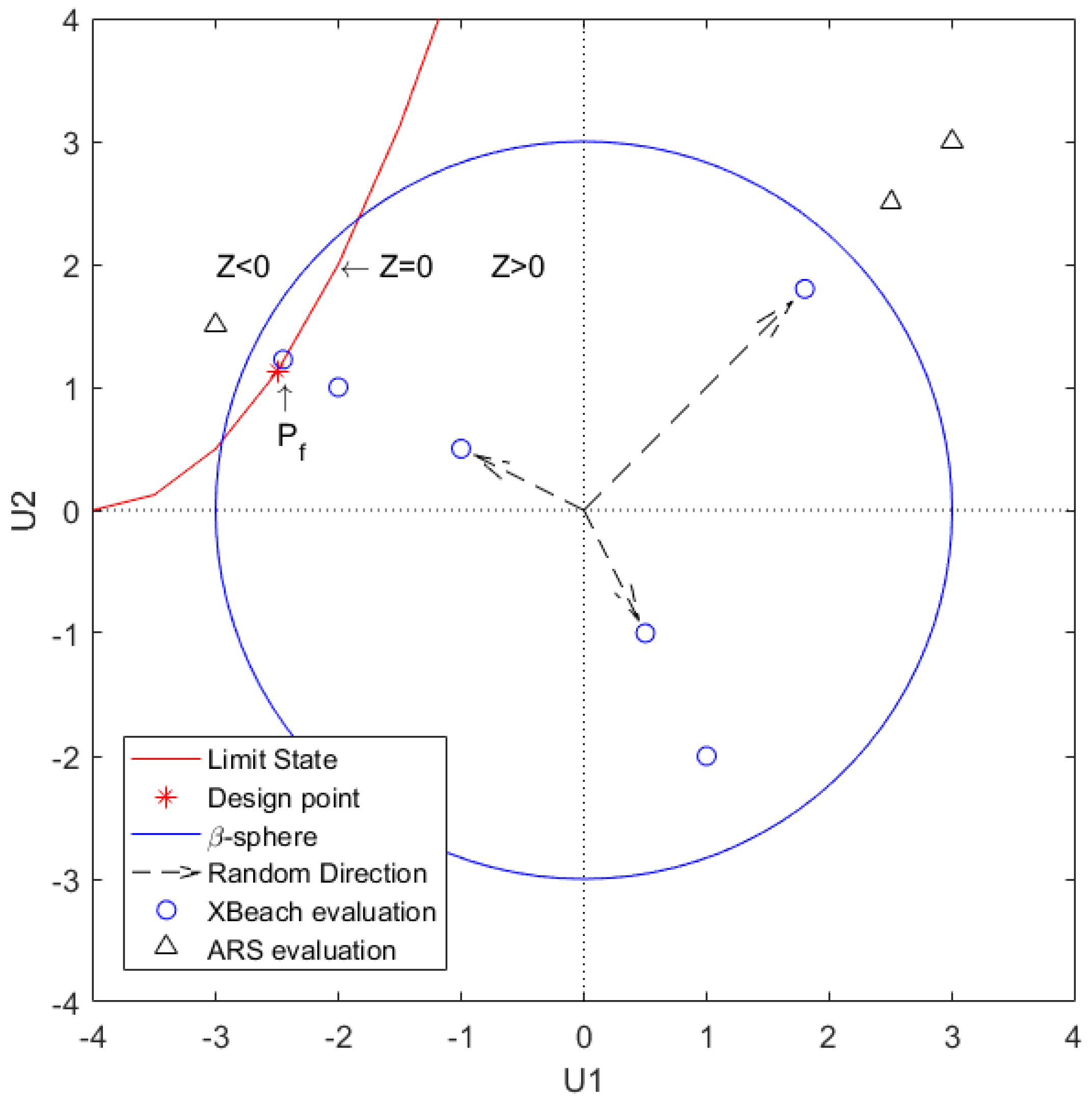
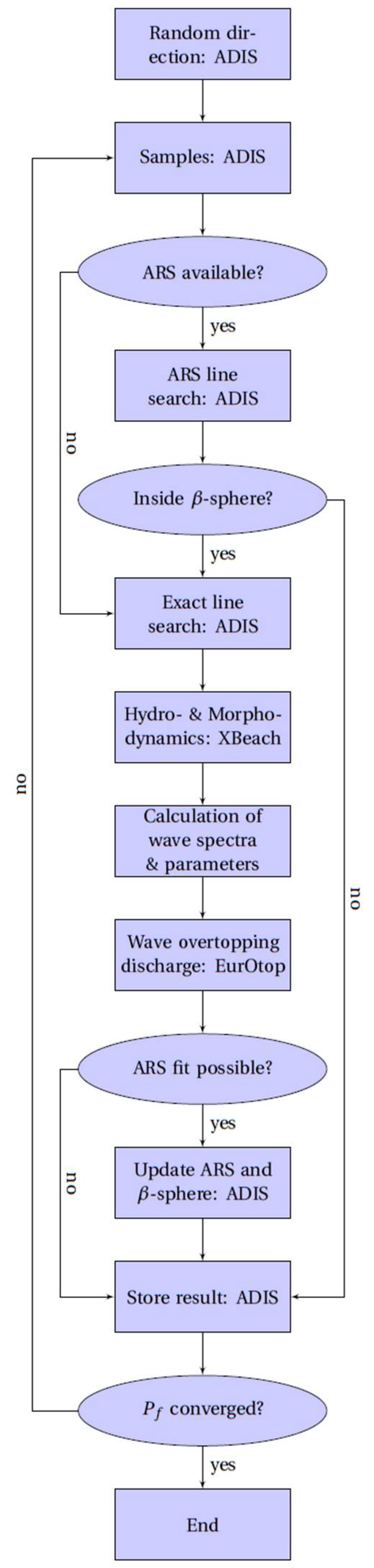
This section gives a description of the probabilistic (ADIS) calculations that were performed with the framework and their results. The influence of the complex hydrodynamics, model and wave parameters, time of the peak of the storm, morphological changes and probabilistic method are described in the sub-sections below.

Table 3. Overview of the different probabilistic (ADIS) calculations that were performed with the framework and their results.

Calc. no. [-]	Type of Model	No. of Stoch. Vars.	Complex Hydrodyn.	Set 1, Offsh. Cond.	Set 2, Model Params	Set 3, Tide, Storm	Set 4, Morph. Changes	Pf [year−1]	β [-]	No. of Simulations [-]	Calc. Duration [days]
1	h/2	3		X				2.3 × 10−8	5.47	23	0.004
2	XB 1D	3	X	X				1.6 × 10−5	4.15	112	1
3	XB 1D	10	X	X	X			2.9 × 10−4	3.45	341	1
4	XB 1D	12	X	X	X	X		1.2 × 10−4	3.67	391	5
5	XB 1D	15	X	X	X	X	X	5.3 × 10−4	3.27	484	7
6	XB 2D	3	X	X				1.6 × 10−6	4.66	43	1

shows an overview of the different probabilistic (ADIS) calculations that were performed with the framework and their results. The table gives the type of hydrodynamic (and morphological) model that was used (column 2), which physical processes were included (columns 4–8), and the resulting number of stochastic variables that were applied (column 3,5–8). Moreover, the resulting probability of failure P_f and the reliability index β are given (columns 9,10), as well as the number of simulations necessary and the calculation duration in days (columns 11,12).

To determine the influence of using a process-based model with complex hydrodynamics compared to a calculation rule, calculations 1 and 2 were performed and will be compared. To determine the influence of including the model and wave parameters as stochastic variables, calculations 2 and 3 will be compared. To determine the influence of including the storm duration and time of the peak of the storm, calculations 3 and 4 will be compared. The influence of morphological changes of the foreshore on the probability of failure due to wave overtopping is determined by comparing calculation 4 and 5.

To determine the influence of the wave directional spreading (short-crested waves), an extra calculation was performed with XBeach 2D and the three offshore conditions as stochastic variables (calculation 6), which is compared to calculation 2.

To determine the added value of using the advanced and fully probabilistic method ADIS as well, the calculated probabilities of failure by the framework were compared to an approach where the same probability exceedance value for each of the stochastic parameters is used (not in table), see Section 3.6.

3.1. Influence of the Complex Hydrodynamics

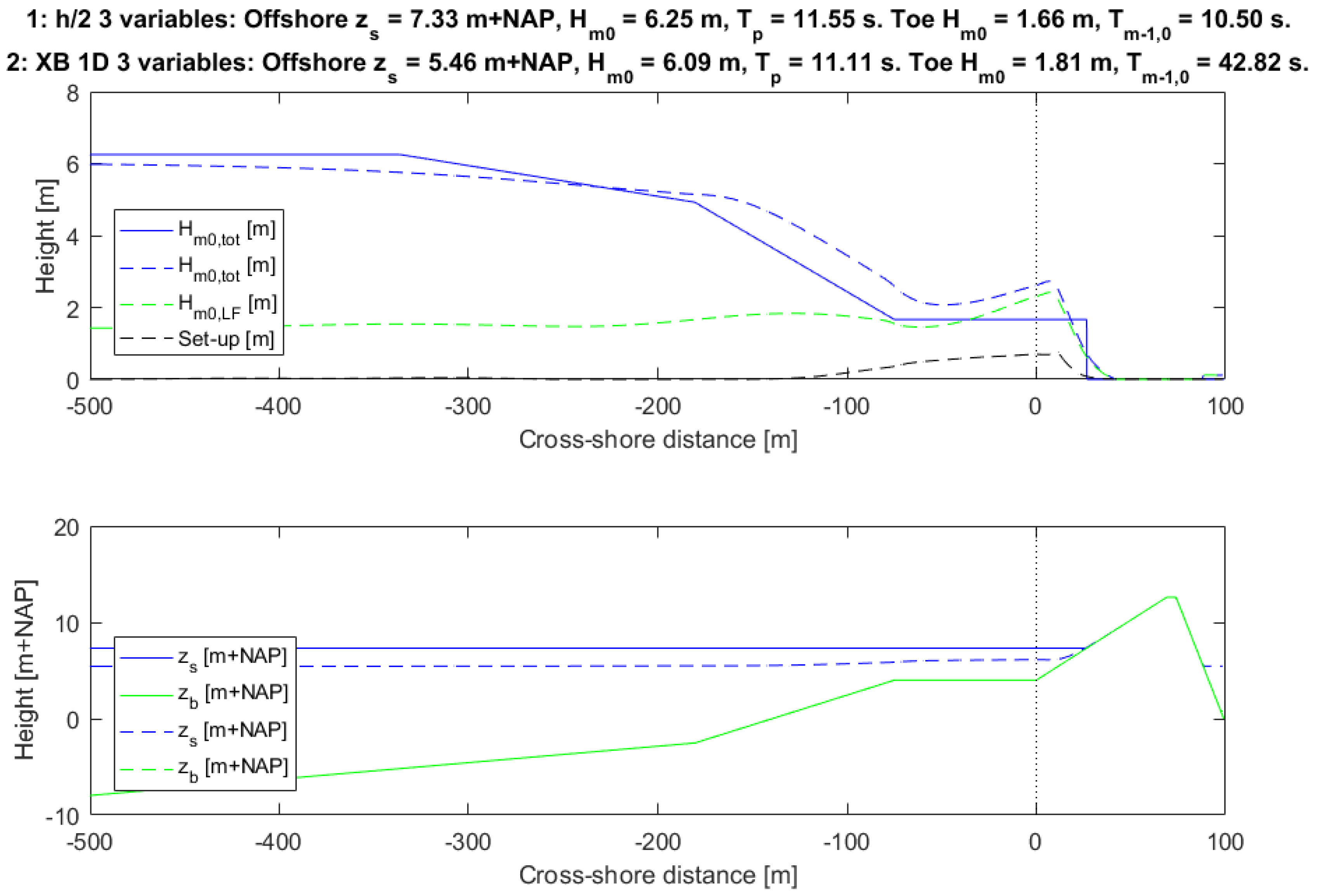
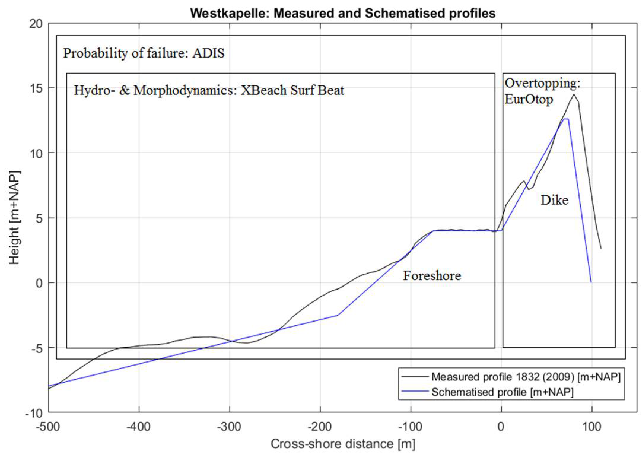
The results of calculations 1 and 2 are shown in Figure 7, comparing the calculation rule h/2-assumption (solid lines) with the process-based model XBeach (dashed lines). The figure shows the results of calculations at the (closest to the) design point. The top plot shows the development of the significant wave height for both situations (blue lines), as well as the low-frequency part of the wave height (green) and wave set-up (black) for XBeach. The bottom plot shows the water levels (blue) and the cross-shore profile (green). The title of the figure gives the conditions offshore and at the toe of the dike for both situations. Note that not the whole profile is visible, but rather the part from −500 m to 100 m relative to the toe of the dike. Using XBeach leads to a much larger failure probability than when the h/2-assumption is used (factor 10³, see Table 3). The dominant parameter in the calculation with the h/2-assumption was the water level, which was very large (7.33 m+NAP), see Figure 7. As can be seen from Figure 7, approximately the same amount of wave overtopping occurs for much less extreme hydraulic conditions (a water level that almost 2 m lower), when including the complex hydrodynamics. The difference in offshore wave height was not as large as for the water level (6.25 m versus 6.09 m). However, the wave set-up in XBeach leads to a somewhat larger wave height at the toe. The main difference lies in the wave period. Offshore, the difference is almost negligible, but due to the inclusion of the wave period transformation and generation of infragravity wave energy, the wave period at the toe is much larger with XBeach. The severe wave breaking on the foreshore leads to a transfer of wave energy to the lower frequencies, which increases the T_m−1,0 wave period strongly (10.50 s versus 42.82 s, see Figure 7). Hence, compared to a calculation rule, using a process-based model that includes complex hydrodynamics like wave set-up, infragravity waves and wave period transformation leads to larger wave heights and much larger wave periods at the toe of the dike. The ratio between the high frequency and low frequency wave heights at the toe (H_m0,HF/H_m0,LF) as calculated by XBeach 1D is only 0.5 in this case. The infragravity waves have a significant contribution to the total wave energy in this 1D case with foreshore. Thus, it can be concluded that it is of importance to include these hydrodynamic processes for these kinds of situations with severe wave breaking on a shallow foreshore. This means that a complex hydrodynamic model is necessary, which further necessitates an efficient probabilistic model.

3.2. Influence of the Model and Wave Parameters

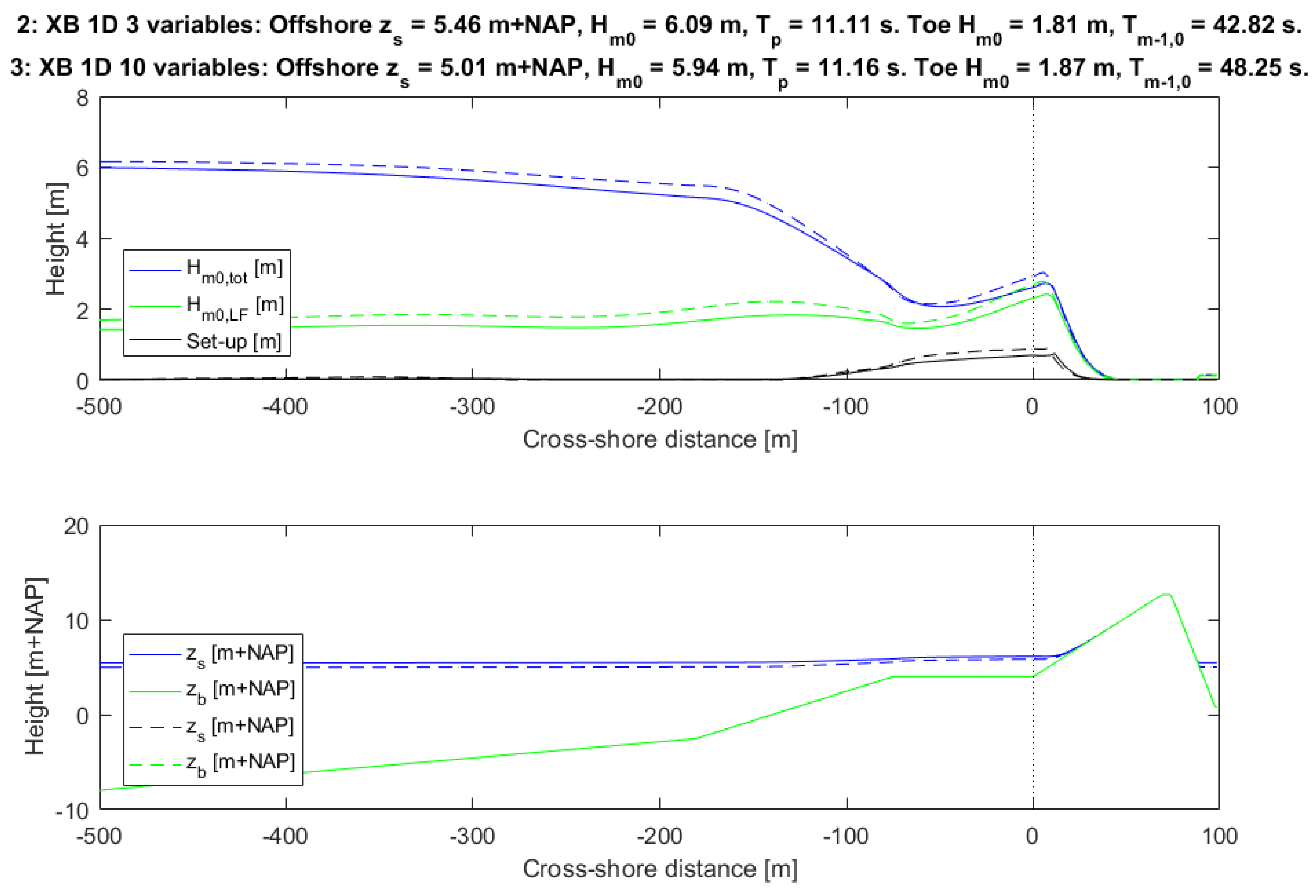
The inclusion of the model and wave parameters as stochastic (10 stochastic variables, calc. 3) leads to a probability of failure that is approximately 20 times larger than the calculation with only stochastic offshore conditions (calc. 2), see Table 3. Hence, the influence is much smaller than the influence of including the complex hydrodynamics such as infragravity waves. The results of calculations 2 and 3 are shown in Figure 8, again showing the calculations in the design point. As can be seen in the figure, a lower water level with approximately the same offshore wave conditions leads to the same amount of wave overtopping in the calculation with 10 stochastic variables, compared to the situation with 3 stochastic variables. The main difference lies in the breaker index γ which is now a stochastic variable. In the design point, the value for this parameter was higher (0.63 versus 0.54 for the deterministic value). This larger breaker index leads to less wave breaking (larger maximum wave height H_max at incipient breaking) and thus larger wave heights at the toe of the dike and more wave overtopping. The difference in probability of failure shows that it can be important to include more stochastic variables than just the offshore conditions. Again, a large wave set-up and strong generation of infragravity wave energy is visible. As a result of this, the T_m−1,0 wave periods at the toe are again quite large. The ratio between the high frequency and low frequency wave heights at the toe (H_m0,HF/H_m0,LF) as calculated by XBeach 1D is only 0.4 in this case. This again shows that it is of importance to include hydrodynamic processes like infragravity waves and wave set-up in the calculations.

3.3. Influence of the Storm Duration and Time of the Peak of the Storm

The next step was to include the storm duration t_storm and time of the peak of the storm ϕ as stochastic variables, leading to a calculation with 12 stochastic variables (calc. 4). Including these parameters as stochastic led to a probability of failure that was approximately 2 times smaller than the calculation with 10 stochastic parameters (calc. 3), see Table 3. Hence, the influence of including these parameters is rather small. The reduction in probability of failure can be explained by the time of the peak of the storm relative to the tide. When this parameter is considered as deterministic, it is assumed that the maximum surge occurs at the same moment as tidal high water. When this parameter is considered stochastic, the moment of maximum surge does not necessarily correspond to the moment of the maximum tidal water level, which reduces the probability of failure. The rest of the stochastic parameter values in the design point of the calculations with 10 and 12 stochastic parameters corresponded almost exactly, which explains the small difference in probability of failure. The small difference in probability of failure shows that for this case, the storm duration and time of the peak of the storm can be neglected as stochastic variables.

3.4. Influence of Morphological Changes

The inclusion of morphological changes of the foreshore during a storm and the corresponding three extra stochastic variables led to a failure probability that was somewhat larger (factor four higher with morphological changes included, see Table 3). The extra stochastic variables, compared to the calculations described in the previous subsections, increased the number of calculations necessary to reach a converged probability of failure. This is a direct result of the inclusion of more parameters, which enlarges the search space (more dimensions).

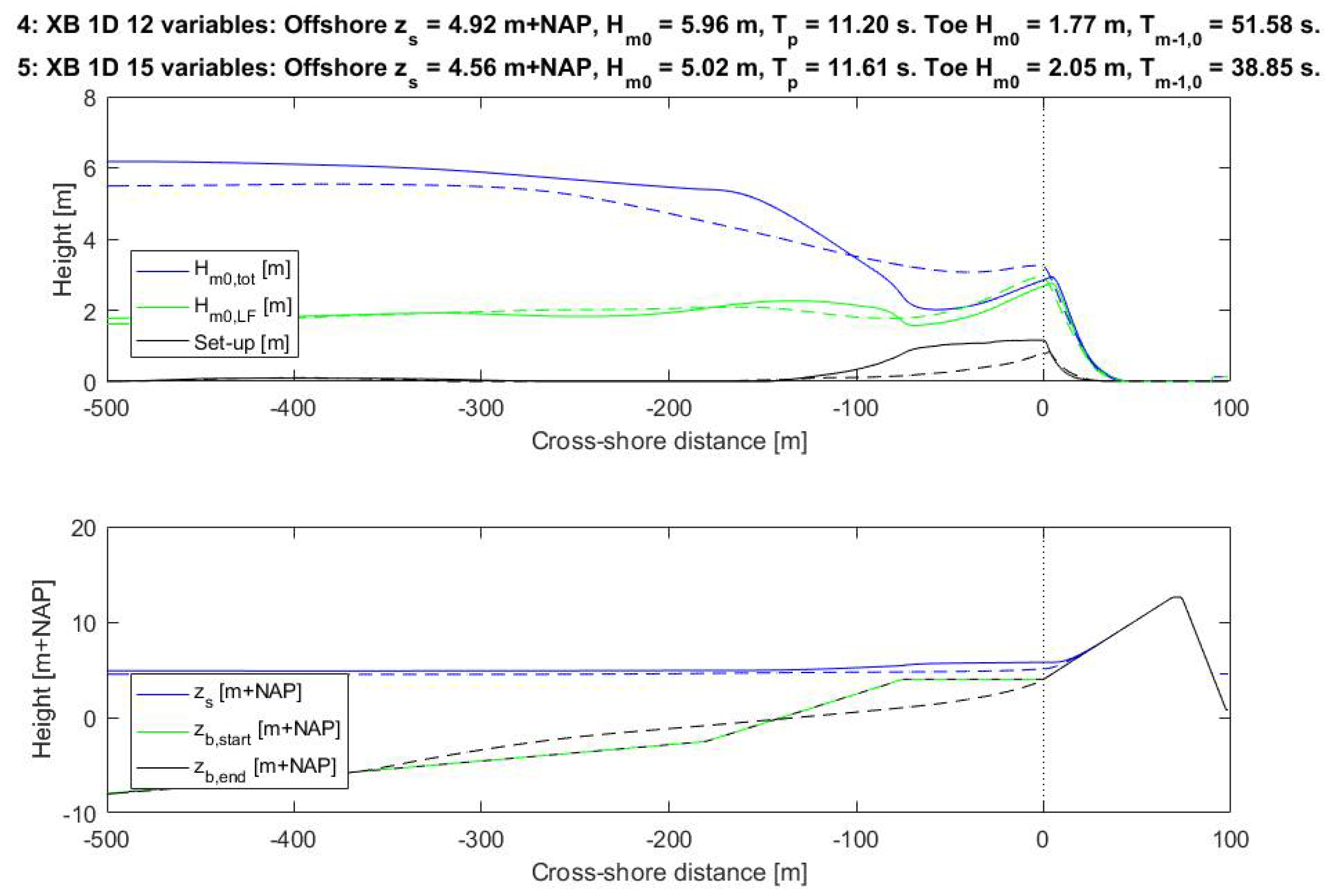
Figure 9 presents the results of the simulations without morphological changes with 12 stochastic variables (calc. 4) and with morphological changes with 15 variables (calc. 5) at the design point. The top plot shows the development of the total significant wave height (blue), the low frequency part of the wave height (green) and set-up (black). The bottom plot shows the water level (blue) and the cross-shore profile at the beginning of the storm (green) and end of the storm (black). The inclusion of morphological changes leads to a somewhat larger probability of failure of about a factor four, as can be seen in Table 3. This change is not very large when compared to the influence of the complex hydrodynamics as infragravity waves and wave set-up for the case considered here. Due to the erosion of the foreshore, the wave dissipation becomes less, which gives larger wave heights at the toe of the dike (2.05 m versus 1.77 m). However, the transfer from high frequency wave energy to the lower frequencies becomes less as well, which gives a smaller T_m−1,0 wave period (38.85 s versus 51.58 s). In this case, the effects of the difference in wave height and wave period almost cancel one another out. This leads to the small difference in probability of failure, despite the quite large differences in the bathymetry due to erosion of the foreshore. Concluding, for this case, the inclusion of the morphological development of the foreshore and related stochastic variables only led to small differences in the probability of failure.

3.5. Influence of Wave Directional Spreading

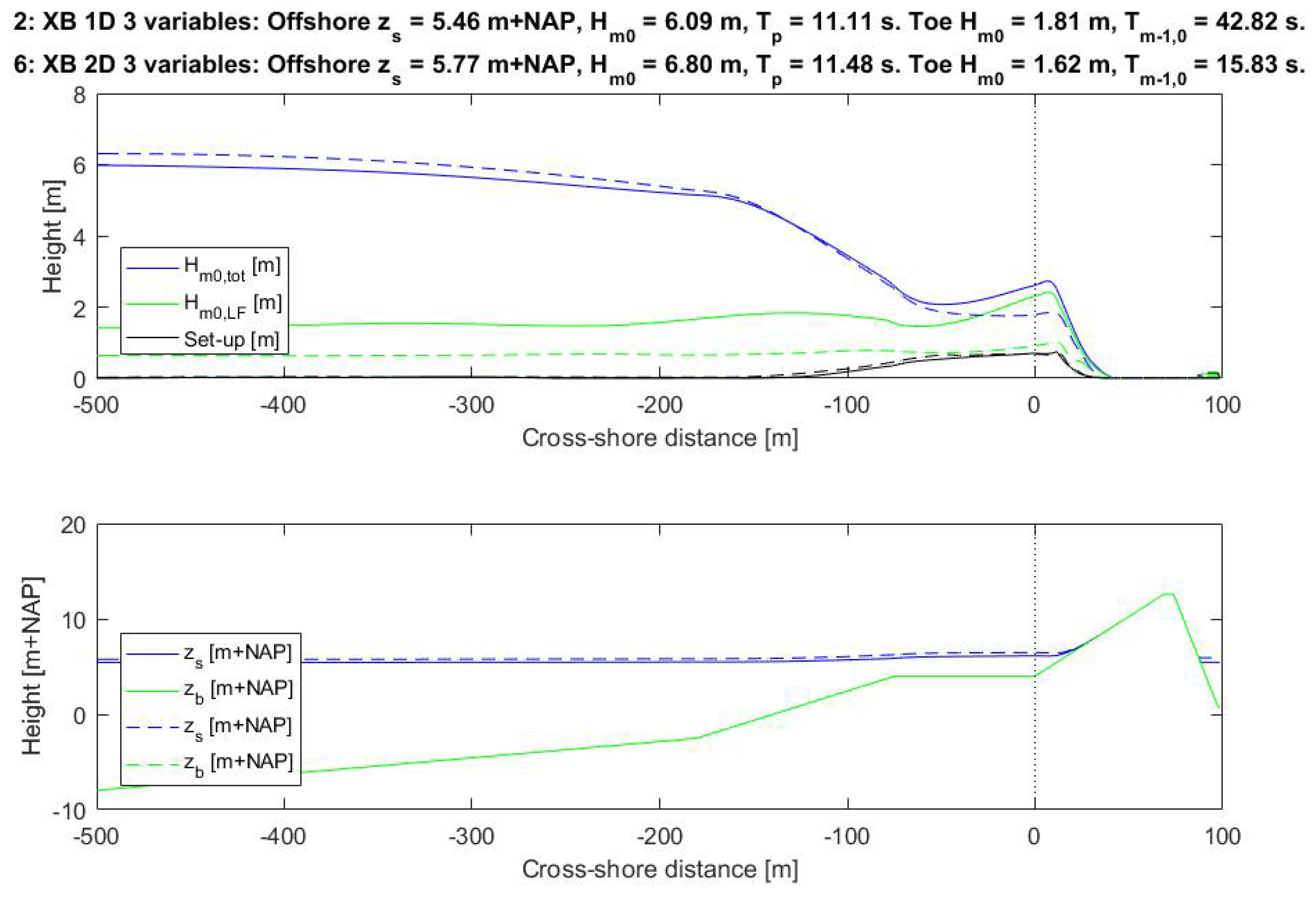
To determine the influence of the wave directional spreading (short-crested waves), an extra calculation was performed with XBeach 2D and the three offshore conditions as stochastic variables (calc. 6), which is compared to XBeach 1D (calc. 2).

As shown in the previous subsection, rather large amounts of low-frequency energy and T_m−1,0 wave periods are found at the toe of the dike when using a 1D simulation. The 1D XBeach calculations can be considered as a wave flume, with long-crested waves without directional spreading. This causes a stronger forcing of the infragravity waves compared to a situation with directional spreading. In reality, wind waves in extreme storms are short-crested. Therefore, an extra calculation was performed with XBeach 2DH with the same three stochastic parameters. With a 2D simulation, the wave directional spreading is included. Thus, the main differences between a 1D and 2D simulation lie within the fact that the 1D simulation does not include the wave directional spreading (hence, long-crested waves), which the 2D simulation does (hence, short-crested waves). For the 2D model, in the alongshore direction, a section of 1 km was modelled with grid cell sizes of 50 m. The wave directional information was solved in 10 degree bins, spanning 110 degrees (55 degrees to both sides of shore normal). Note that the mean wave angle in all simulations was shore-normal and that we use the methodology of Roelvink et al. [34] to resolve the propagation of wave groups in the model domain. The results are shown in Figure 10.

The calculated probabilities of failure are 1.6 × 10⁻⁵ for the 1D case and 1.6 × 10⁻⁶ for the 2D case, a difference of a factor 10. The lower probability of failure as found for the 2D case can be explained by the forcing of the infragravity waves, which is less than in the 1D case, because the 2D XBeach calculations include the wave directional spreading. This leads to less low-frequency energy and therefore a smaller wave period at the toe (15.83 s versus 42.82 s), which results in less wave overtopping. For instance Hofland et al. [11] show as well that the generation of low-frequency wave energy is decreased by the directional spreading. With the inclusion of the wave directional spreading, the results of a 2D simulation are more realistic compared to a 1D simulation, since wind waves in extreme storms are short-crested (see also e.g., Van Dongeren et al. [50]). The ratio between the high frequency and low frequency wave heights at the toe (H_m0,HF/H_m0,LF) is 1.6 for the 2D case (compared to 0.5 for the 1D case). Thus, even in 2D the infragravity waves have a significant contribution to the total wave energy.

3.6. Influence of the Probabilistic Method

The influence of using the level III probabilistic method ADIS on the number of simulations necessary was determined before in Section 2.2.3., as well as in Den Bieman et al.; Grooteman [21,36]. An indication of the added value of using this level III method can be gained by comparing the ADIS results with probabilistic calculations that use the same probability exceedance value for each of the stochastic parameters. This means that the stochastic parameters are considered as fully correlated. This was done for XBeach 1D with the three offshore condition parameters (water level, wave height and wave period) as stochastic variables. The results are given in

Table 4. Comparison of the probabilities of failure as calculated with ADIS and as calculated with an approach that uses the same probability exceedance value for each of the stochastic parameters (fully correlated). Results for XBeach 1D with the three offshore parameters as stochastic variables.

Calculation	Offshore zs [m+NAP]	Offshore Hm0 [m]	Offshore Tp [s]	Toe Hm0 [m]	Toe Tm−1,0 [s]	Pf [year−1]	β [-]
XBeach 1D fully correlated	5.16	6.32	11.74	1.84	46.62	2 × 10−4	3.54
XBeach 1D ADIS	5.46	6.09	11.11	1.81	42.82	1.6 × 10−5	4.15

. It can be seen that a difference of a factor 12.5 in the probability of failure is found between ADIS and the fully dependent estimate. Hence, when using a level III fully probabilistic approach, a lower probability of failure and a lower required crest height of the dike are found. It can be imagined, that if more stochastic variables would be included in this comparison, the difference between the estimate and the advanced probabilistic approach would be even larger. Thus, using ADIS in the design of dike-foreshore systems can lead to lower required crest levels.

4. Discussion

The calculation duration of some of the probabilistic calculations was rather large, in the order of a day without morphological changes (either 1D or 2D), in the order of a week (1D) with morphological changes, on 8 nodes with 16 GB of RAM. For this paper, the calculations with large numbers of stochastic variables and morphological changes were only performed with XBeach 1D. With the current computational capacities, using XBeach 2D and including the morphological changes in the probabilistic framework is not feasible in an engineering context yet, but it is for an academic context. As shown before, for the present case the morphological response has a relatively small influence on the failure probability. As the morphological response is expected to become lower when using a 2D calculation with short-crested waves, this will further decrease the influence of morphology on the failure probability, a consequence of the decreased infragravity wave height. With increasing computational power, the feasibility of XBeach 2D will likely increase in the future. As well, a possible measure could be to use a morphological acceleration factor in XBeach. Also, recently, a prediction formula for the T_m−1,0 on mildly sloping shallow foreshores was determined [11]. This equation can be used for simple cross-shore profiles and could be implemented in the model framework to save calculation time for such cases. For more complex cross-shore profiles, XBeach will remain necessary.

In the calculations with morphological changes, XBeach created a characteristic storm profile with an offshore bar, the foreshore itself was largely eroded. As mentioned before, XBeach has been extensively calibrated and validated [26,27]. However, even if the calculated offshore bar height would not be completely correct, this would hardly affect the wave conditions at the toe and related overtopping discharge. Van Gent & Giarrusso [15] found that the wave conditions at the toe of the structure are hardly affected by the level of the offshore bar (and/or trough), but are strongly affected by the level of the foreshore.

As mentioned before, the focus of this paper is on the dominant short term storm morphological changes, not on the long term changes by the daily climate. The bathymetrical profile after the storm with conditions corresponding to the parameter values in the design point was compared to the bathymetrical profiles at Westkapelle 1 year after construction of the foreshore and 5 years after construction of the foreshore. The morphological changes of the ‘design point storm’ were much larger than the changes by the daily climate after five years. This does not mean that the after-storm erosion profile of a pre-storm situation with a foreshore without much sand in it is the same as the erosion profile for a pre-storm situation with much sand in the foreshore. For maintenance, this means that the design foreshore profile should be maintained as much as possible. Furthermore, it is expected that the role of short term (storm) changes of the foreshore become more important when the foreshore is designed smaller (less sand in the profile). Finally, these findings are case-specific. At other locations, there may be more or less dynamic behavior, and also the ratio between the erosion by daily and storm conditions can vary.

Much of the validation for wave overtopping was performed in wave flumes (1D, no directional spreading), which inherently includes the stronger forcing of the infragravity waves, like in XBeach 1D. As was shown, a large part of the difference in the results between 1D and 2D XBeach was caused by differences in the T_m−1,0 wave period at the toe and uncertainties in the sensitivity of the EurOtop equations with respect to this wave period. Since the T_m−1,0 wave period is very sensitive to the low frequencies, it is unclear if this wave period is still applicable for situations with large amounts of low frequency energy, such as the ones considered in this paper. Treating the complex combination of infragravity wave energy and wind wave energy with a single parameter as the T_m−1,0 wave period might be an oversimplification, however the T_m−1,0 wave period is the wave period that is currently used in all the most commonly used wave run-up and wave overtopping equations. A new equivalent slope concept was determined for wave overtopping at shallow foreshores in Altomare et al. [51] and could be considered a first step. However, still more research is required to be able to validate the influence of the infragravity waves on wave overtopping, for this case, as well as for other cases.

5. Conclusions

This paper presented a probabilistic model framework which is capable of including complex hydrodynamics like infragravity waves and morphodynamics of a sandy foreshore in the calculation of the probability of sea dike failure due to wave overtopping. The method was applied to a test case loosely based on the Westkapelle sea defence, a hybrid defence consisting of a dike with a sandy foreshore. Moreover, the influence of the physical processes like infragravity waves and morphological changes on the probability of dike failure due to wave overtopping were determined. By using the fully probabilistic level III method ADIS, the number of simulations necessary is greatly reduced, which allows for the use of more advanced and detailed hydro- and morphodynamic models. The framework is able to compute the probability of failure with up to 15 stochastic variables and to describe feasible physical processes. Furthermore, the framework is completely modular, which means that any model or equation can be plugged into the framework, whenever updated models with improved representation of the physics or increases in computational power become available.

The model framework as described in this paper, includes more stochastic variables in the determination of the probability of dike failure due to wave overtopping compared to the currently used methods in the Netherlands, where also infragravity waves or morphological changes are not included.

Including a process-based hydrodynamic model led to much larger failure probabilities for the hybrid defence considered in this paper (factor 10³). This difference was mainly caused by the difference in wave period at the toe of the dike, which is not accounted for by the simple calculation. Hence, this indicates that it can be important to include the complex hydrodynamics such as infragravity waves and wave set-up for these kinds of situations.

The inclusion of 7 extra stochastic model and wave parameters led to a probability of failure that was approximately 20 times larger than the calculation with 3 offshore condition stochastic parameters. The influence is much smaller than the influence of including the complex hydrodynamics such as infragravity waves, but the difference in probability of failure shows that it can still be important to include more stochastic variables than just the offshore conditions in the calculations. Furthermore, for this case the storm duration and time of the peak of the storm have a negligible influence as stochastic variables.

The inclusion of the morphological changes led to a failure probability that was only somewhat larger (factor 4) for the case considered here (relative to e.g., the much larger influence of the complex hydrodynamics that was found). Hence, for this case, the influence of the morphological changes of the foreshore on the failure probability was not that large. In this case, the effects of the difference in wave height and wave period at the toe almost cancelled one another out.

More research is required to be able to validate the influence of the infragravity waves on wave overtopping, for this case, as well as for other cases, especially in connection to short-crested waves. The results of a 2D simulation are more realistic compared to a 1D simulation, see also e.g., Van Dongeren et al. [50], as wind waves in extreme storms are short-crested. The long-crested waves in XBeach 1D create a stronger forcing of the infragravity waves. With the current computational capacities, a 2D calculation and including the morphological changes in the level III probabilistic framework is not feasible in an engineering context yet, but it is for an academic context. With increasing computational power, the feasibility will likely increase in the future.

Using the framework offers more insight into the physics, and can be used to determine the contribution of foreshores to flood protection. It is recommended to apply the framework to other cases as well, to determine if the effects of complex hydrodynamics as infragravity waves and morphological changes on the probability of sea dike failure due to wave overtopping as found in this paper hold for other cases as well. Furthermore, it is recommended to investigate broader use of the method, e.g., for safety assessment, reliability analysis and design.