A Semi-Empirical Prediction Method for Broadband Hull-Pressure Fluctuations and Underwater Radiated Noise by Propeller Tip Vortex Cavitation ^†

Abstract

A semi-empirical method is presented that predicts broadband hull-pressure fluctuations and underwater radiated noise due to propeller tip vortex cavitation. The method uses a hump-shaped pattern for the spectrum and predicts the centre frequency and level of this hump. The principal parameter is the vortex cavity size, which is predicted by a combination of a boundary element method and a semi-empirical vortex model. It is shown that such a model is capable of representing the variation of cavity size with cavitation number well. Using a database of model- and full-scale measured hull-pressure data, an empirical formulation for the maximum level and centre frequency has been developed that is a function of, among other parameters, the cavity size. Acceptable results are obtained when comparing predicted and measured hull-pressure and radiated noise spectra for various cases. The comparison also shows differences that require adjustments of parameters that need to be further investigated.

1. Introduction

Noise and vibration on board ships are important design considerations for the comfort of crew and passengers. High comfort levels are especially required by passengers on cruise vessels and owners of yachts. An important source affecting comfort is cavitation on the ship propeller. The collapse of cavitation generates pressure fluctuations that excite the ship hull above the propeller leading to on board noise and vibration. The reduction of cavitation-induced noise and vibration is usually achieved by unloading the propeller tip and decreasing sheet cavitation as much as possible, often leaving only tip vortex cavitation on the propeller. However, this type of cavitation generates low-frequency broadband hull-pressure fluctuations that may lead to ship vibration issues [1,2].

The cavitating propeller is also an important contributor to the underwater radiated noise (URN) of ships. URN is relevant for the acoustic signature of military ships, for the operation of equipment that require low self-noise such as sonar, and for the influence on marine life. The latter used to be relevant for fishery research vessels only, but, in the last decade, the impact on the marine environment of URN due to shipping in general has received considerable attention. URN by shipping is included in the environmental descriptors to achieve Good Environmental Status of European Seas in the EU Marine Strategy Framework Directive (2008/56/EC), The International Maritime Organization (IMO) has released in 2013 non-mandatory guidelines for the reduction of underwater noise from commercial shipping, and class societies DNV-GL, BV, RINA and LR have developed rules for URN of commercial ships.

The spectrum of the broadband hull-pressure fluctuations is characterized by a hump, the maximum level of which increases with ship speed, while the centre of the hump simultaneously moves to lower frequencies. This centre frequency is typically located between 30 Hz and 200 Hz. A possible explanation of the hump in the spectrum is that it is caused by a resonance frequency of the cavitating vortex [3], although experimental evidence of this is missing. The proposed criterion for resonance assumes zero group speed in the dispersion relation for cavitating vortices. Experimental evidence for this dispersion relation is presented in [4] in which further support for the criterion for resonance is also given. The relation between the broadband part and the blade rate tonals in the hull pressure spectrum is briefly discussed in [5].

It has been shown that the source level of URN due to propeller cavitation has a direct relation with the pressure levels on the hull [6,7]. Source levels can directly be estimated from measured hull pressures by correcting the hull pressures for the solid boundary factor on the hull and the distance between cavity collapse and pressure sensor. These source levels are in reasonable agreement with source levels obtained by hydrophone measurements in the far field of the ship.

The hull-pressure fluctuations and URN can be predicted in model test facilities [8,9,10,11,12] to evaluate propeller designs. CFD methods are rapidly developing but are still computationally expensive and not yet mature enough in this area to be used in the iterative design procedure. Rapid evaluation of propeller designs usually relies on the use of potential flow methods that can predict sheet cavitation and the resulting hull-pressure fluctuations and URN at the blade passage frequency [13,14,15]. The sheet cavitation extents and dynamics can also be used in semi-empirical methods to predict the related broadband URN [16,17]. Because vortices are fitted rather than captured when using potential flow methods, alternative methods are required to predict developed vortex cavitation. The results of the potential flow method can be used in computational noise prediction methods that solve a two-dimensional Rayleigh-Plesset type of equation for a vortex cavity segment [18,19,20] or that make use of a semi-empirical model [21,22].

The present paper proposes a semi-empirical method to predict the broadband hull pressure fluctuations and URN by propeller tip vortex cavitation that can easily be used in the propeller design process. The method is based on the semi-empirical method to predict on board noise of cavitating tip vortices by Raestad [21]. This method relates the noise to the size of the vortex cavity that is estimated from a potential flow method. In the present method, use is made of the boundary element method (BEM) PROCAL [14,23,24] to estimate the vortex strength (circulation) of the tip vortex. This strength is used in a vortex model for the radial distribution of the azimuthal velocity to predict the cavity size for a given cavitation number. The vortex model and cavity size prediction are discussed in Section 2.1 and Section 2.2, respectively. The predicted cavity size has been used in an empirical relation for the centre frequency and maximum level of the broadband hump. This procedure is presented in Section 2.3. A flow chart of the method is shown in Figure 1. The spectral shape of the source level spectrum and conversion to hull pressure spectrum and URN spectrum is presented in Section 3. Comparison of predicted and measured spectra is presented in Section 4. The results of the method are discussed in Section 5.

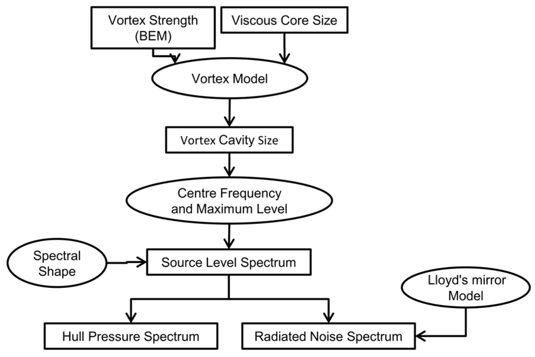
2. Prediction of the Maximum Source Level

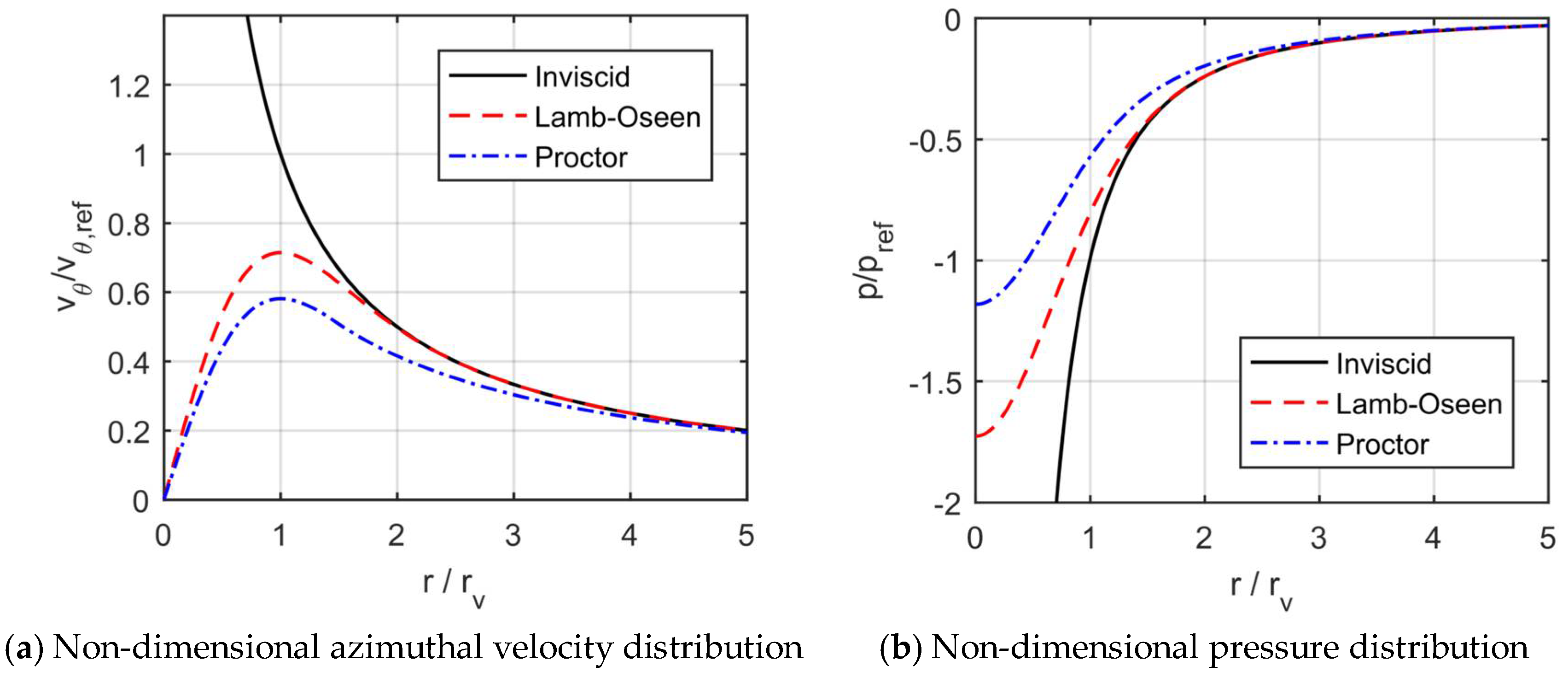
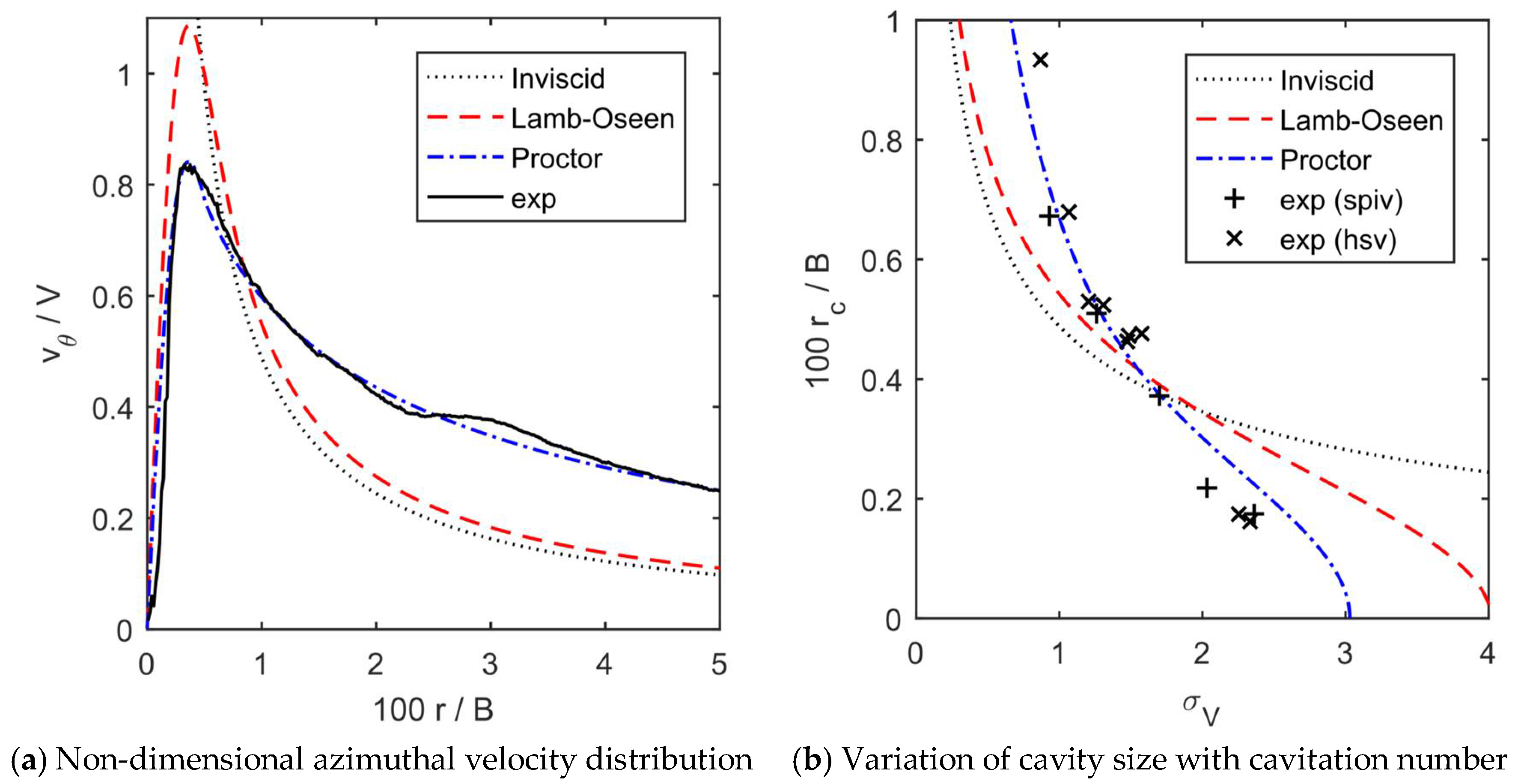
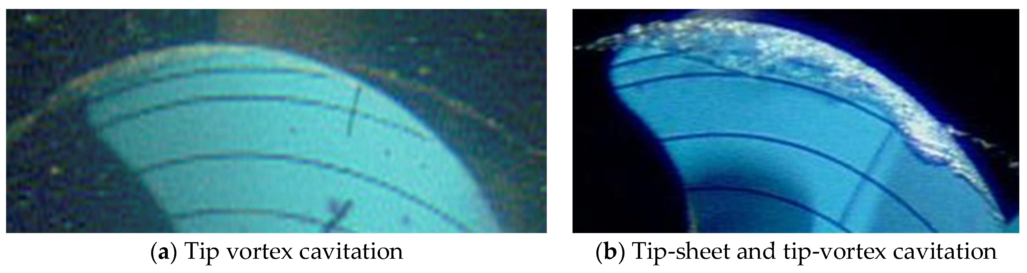
2.1. Vortex Models

The relation between cavitation number and cavity size for a vortex cavity can be obtained from the radial distribution of the azimuthal velocity $v_{\theta }$. It has been shown [25] that the variation of pressure $p$ with radius $r$ can be computed within 10 to 15% accuracy using the relation

$$p-p_{\infty }=-{\displaystyle \underset{r}{\overset{\infty }{\int }}\rho \frac{v_{\theta }^2}{r}}\hspace{0.17em}dr.$$

(1)

Theoretical analysis has shown that the variation of cavity size with cavitation number for an analytical solution of a columnar cavitating vortex is almost identical to that of a non-cavitating vortex if the viscous core size does not change [26]. For the non-cavitating vortex, the cavity radius was taken as the radius where pressure equals vapour pressure. Therefore, only non-cavitating vortex models will be considered in the following.

The most simple vortex model is the potential flow vortex of which the azimuthal velocity is given by

$$v_{\theta }\left(r\right)=\frac{{\mathsf{\Gamma }}_{\infty }}{2\pi r},$$

(2)

where ${\mathsf{\Gamma }}_{\infty }$ corresponds to the vortex strength, which is defined as the circulation $\mathsf{\Gamma }$ at large $r$. A disadvantage of this model, referred to in the following as inviscid vortex, is the singular behavior at the centre, which leads to an infinitely low pressure at that location. In real flow, this singular behavior does not appear due to viscous effects. An analytical solution for a columnar vortex in laminar flow is the Lamb–Oseen vortex [27] with viscous core radius $r_v$,

$$v_{\theta }\left(r\right)=\frac{{\mathsf{\Gamma }}_{\infty }}{2\pi r}\left\{1-\exp \left[-\varsigma {\left(r/r_v\right)}^2\right]\right\}.$$

(3)

The parameter $\varsigma$ is a constant that is selected such that $v_{\theta }$ has its maximum value at $r=r_v$, which gives $\varsigma =1.2564$. The Lamb–Oseen vortex can be interpreted as the solution of a potential flow vortex of which the vorticity has been distributed by diffusion. For tip vortices, the distribution of vorticity is also influenced by the roll-up of the trailing vortex sheet that is generated by the spanwise circulation distribution on wing or propeller. The velocity distribution resulting from such a process has been proposed by Proctor et al. [28] and is given by

$$v_{\theta }\left(r\right)=\{\begin{array}{cc}1.0939\frac{{\mathsf{\Gamma }}_{\infty }}{2\pi r}\left\{1-\exp \left[-\beta {\left(1.4\hspace{0.17em}{r}_v/B\right)}^p\right]\right\}\left\{1-\exp \left[-\varsigma {\left(r/r_v\right)}^2\right]\right\}\hfill & r\le 1.4\hspace{0.17em}{r}_v\hfill \\ \frac{{\mathsf{\Gamma }}_{\infty }}{2\pi r}\left\{1-\exp \left[-\beta {\left(r/B\right)}^p\right]\right\}\hfill & r>1.4\hspace{0.17em}{r}_v\hfill \end{array}\hspace{1em}.$$

(4)

In this formulation, $B$ is the length scale related to the vorticity roll-up region, taken as the wingspan of the aircraft by Proctor. The parameters $\beta$ and $p$ are non-dimensional empirical parameters, which take the values $\beta =10$ and $p=0.75$. The variation of the azimuthal velocity with radius is presented in Figure 2a and the corresponding pressure distribution is presented in Figure 2b. The parameter $B$ was taken as $B/r_v=20\hspace{0.17em}.$

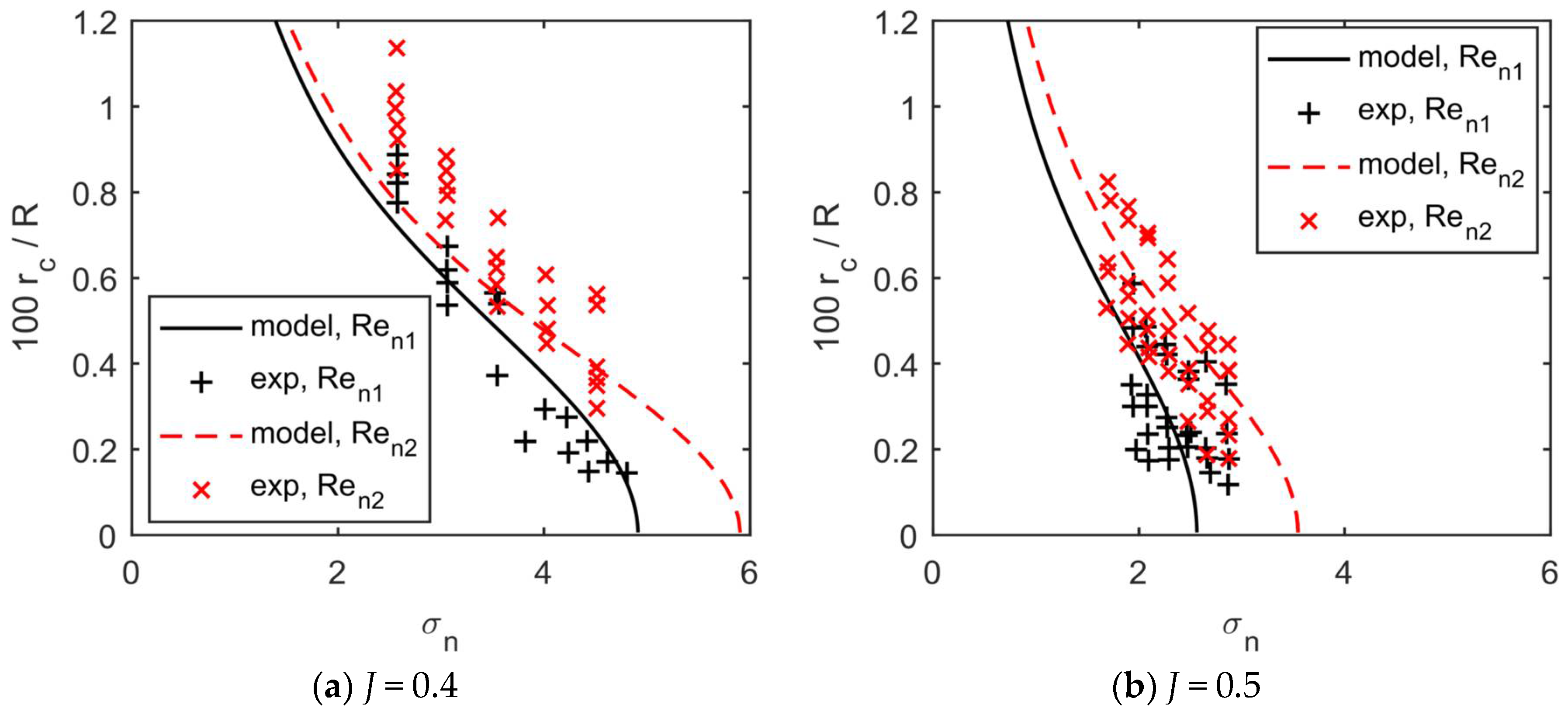
2.2. Prediction of Cavity Size

The vortex models described in Section 2.1 have been evaluated using experimental datasets for a wing, Pennings et al. [29], and for a propeller, Kuiper [30]. The dataset for the wing consists of velocity measurements obtained with stereo particle image velocimetry (spiv) at several stations downstream of the tip and of vortex cavity size measurements as a function of cavitation number ${\sigma }_V$,

$${\sigma }_V=\frac{p_w-p_v}{\frac{1}{2}\rho V^2},$$

(5)

with $p_w$ the static pressure at the location of the wing, $p_v$ the vapour pressure and $V$ the free-stream velocity of the cavitation tunnel. The cavity size was obtained from image analysis using high speed video (hsv). The wing was of elliptical planform (half-span $B/2=0.15\hspace{0.17em}\mathrm{m}$) and tested at three angles of attack. The velocities were averaged in the circumferential direction and the resulting azimuthal velocity distribution for 7 deg angle of attack is presented in Figure 3a, which also shows the results of the vortex models. In these models, $r_v$ was taken as the radius at which the measured $v_{\theta }$ has the maximum value. The Proctor vortex is capable of describing the measured velocity distribution very well after adjusting the coefficients for $\beta$ and $p$. The strength for the Proctor vortex was set to 80% of the maximum value of the spanwise circulation distribution on the wing. This maximum value can be computed from the measured lift coefficient assuming that the circulation distribution is given by the analytical formulation. The resulting variation of $r_c$ with ${\sigma }_V$ of the Proctor vortex also shows very good agreement with experimental data, as shown in Figure 3b. The inviscid and Lamb–Oseen vortex do not describe the velocity distribution and the cavity size variation well. In the results shown, the vortex strength for these vortices has been adapted such that the average cavity size is well predicted. It is remarked that the good prediction of the variation of cavity size with cavitation number by a vortex model for non-cavitating flow is not understood from a physical point of view. Experiments for cavitating flow suggest that the viscous core size used in the vortex model changes in the presence of cavitation, which results in a different prediction of the cavity size [26].

The data set for the propeller consists of the variation of $r_c$ with cavitation number ${\sigma }_n$,

$${\sigma }_n=\frac{p_s-p_v}{\frac{1}{2}\rho n^2{D}^2},$$

(6)

with $p_s$ the static pressure at the shaft centre, $n$ the shaft rotation rate [rev/s] and $D$ the propeller diameter. The propeller was four-bladed, specifically designed to show tip vortex cavitation only, and has diameter $D=0.34\hspace{0.17em}\mathrm{m}$ and pitch ratio $P_{0.7}/D=0.74$. The propeller was tested in open water conditions at three advance ratios by varying the free-stream velocity of the cavitation tunnel. The advance ratio $J$ is defined as $J=V/nD$. Each advance ratio was tested at two shaft rotation rates resulting in two different Reynolds numbers. The Reynolds number was defined as ${\mathrm{Re}}_n=n{D}^2/\nu$, with $\nu$ the kinematic viscosity.

The cavity size was estimated using image analysis of photographs. Roughness was applied on two blades, except at the leading edge to investigate its effect and two blades were kept smooth. However, the geometry of one of the smooth blades differed from the other blades and results for this blade were excluded from the comparison. Overall, the change in cavity size due to the application of roughness, as well as due to variations of air content in the tunnel, was within the measurement uncertainty so the effect could not be determined.

For the present method, the tip-vortex strength was obtained from the circulation computed by PROCAL at 0.95R, with $R=D/2$, and the viscous core size was obtained from model-scale measurements by Jessup [31] scaled according to Equation (7), which is discussed later. Results are shown for the Proctor vortex model only. Initially, the values for $\beta$ and $p$ were kept identical to the values obtained for the wing, but these did not result in a good agreement with experimental data. This indicates that the vorticity roll-up of the wake of the propeller differs from that of the wing. A new tuning process was then applied for β and $p$, which resulted in a reasonable agreement with experimental data, as shown in Figure 4. The variation in Reynolds number in the experiments results in a variation in $r_v$ in the vortex model. In the present method, this dependency was taken into account by using the Reynolds number scaling for cavitation inception of McCormick [32]. The viscous core size can then be computed from the measured value by Jessup [31] referred to as ref,

$$\frac{r_v}{c}={\left(\frac{r_v}{c}\right)}_{ref}{\left(\frac{\mathrm{Re}}{{\mathrm{Re}}_{ref}}\right)}^{-m/2},$$

(7)

with $c$ the chord length and $\mathrm{Re}$ the Reynolds number for the chord length and the resultant velocity at 0.95R. The value for parameter $m$ is computed using the formulation by Shen et al. [33] resulting in a value of 0.38 and 0.37 for the lower and higher Reynolds number, respectively. The effect of the change in Reynolds number on cavity size is well predicted by this method. The vortex model shows that the effect of the viscous core size on the cavity size decreases with increasing cavity size, as shown in Figure 4a.

Results were also analyzed for other angles of attack for the wing and other advance ratios for the propeller. Good agreement was obtained for the other two angles of attack of the wing (5 and 9 deg) using the same settings for the vortex model (see also [26]). However, for the lowest advance ratio of the propeller, $J=0.3$, and hence the case with highest vortex strength, the predicted cavity size was smaller than observed by experiments. A possible reason for this underprediction is that, in the experiment, a combination of sheet and vortex cavitation was present. Unfortunately, no detailed images are available for these conditions so this has not been further investigated.

2.3. Prediction of Source Levels

The semi-empirical formulation for the centre frequency and level of the hump was developed using non-dimensional parameters. In the present study, use has been made of a combination of model-scale, measured in the Depressurized Wave Basin (DWB), and full-scale experimental data for hull pressures obtained for twin-screw vessels. The rms-pressure amplitudes were converted into k_p-values according to Equation (8), where $\Delta f$ corresponds to the resolution bandwidth of the amplitude spectrum and $f_{bpf}$ to the blade passage frequency. The levels were converted to decibel values according to Equation (9). The frequencies were made non-dimensional with $f_{bpf}$:

$$k_p=\frac{p_{rms}}{\rho n^2{D}^2\sqrt{\Delta f/f_{bpf}}},$$

(8)

$$k_p\left[dB\right]=120+20{\log }_{10}\left(k_p\right).$$

(9)

The resulting spectrum can then be interpreted as a non-dimensional power density spectrum or non-dimensional rms amplitude density spectrum. The hull-pressure spectra were converted to source levels by correcting for the propeller-hull clearance and the solid boundary factor. Only the centre pressure sensor located directly above the 12 o’clock position of the propeller was considered, as measurements at this location were available for all data sets.

To focus on the broadband character, the spectrum was converted to 1/6 octave band levels and scaled back to a power density spectrum, an example of which is given in Figure 5. The resulting spectrum then becomes a smoothened power density spectrum. Next, the centre frequency, the maximum level and the bandwidth of the hump were determined by a curve fit. In Figure 5, the centre frequency was determined at $f_c/f_{bpf}=7.3$.

The parameters for the semi-empirical model are the cavity size $r_c$ made non-dimensional with diameter D, the cavitation number ${\sigma }_n$ and the number of blades Z. The empirical relation for the maximum level, which equals the level of the hump centre, is given by

$$k_{p,\max }=a_p+\hspace{0.17em}20{\log }_{10}\left\{{\left(\frac{r_c}{D}\right)}^{\kappa }\sqrt{Z}\right\},$$

(10)

in which the non-dimensional empirical constants $a_p$ and $\kappa$ were obtained by curve fitting of Equation (10) to the experimental data. Raestad [21] has used $\kappa =2$ in his formulation, but the value $\kappa =3$ is used in the present method as this is closer to the trend seen in the datasets. The contribution from the total number of blades is summed as a set of incoherent sources. The formulation for the centre frequency is based on theoretical considerations and is given by

$$\frac{f_c}{f_{bpf}}=b_f\hspace{0.17em}\hspace{0.17em}\frac{1}{r_c/D}\frac{\sqrt{{\sigma }_n}}{Z},$$

(11)

with $b_f$ a non-dimensional empirical constant. Raestad derives this relation from the resonance frequency of a bubble, although the relation has also been derived from the dispersion relation for a cavitating vortex [3].

The vortex strength for the vortex models was obtained from the maximum circulation value at 0.95R of all blade positions computed by PROCAL using model-scale measured wake fields. For the analysis of sea trial conditions, these wake fields were scaled using a method developed in a Cooperative Research Ships (CRS) working group [34]. This method decomposes the ship wake into the contribution from the hull boundary layer and from the wake of struts and shaft, and scales these components separately using semi-empirical formulations.

The ships in the experimental dataset used to derive Equations (10) and (11), and to determine the empirical constants $a_p,$ $\kappa$ and $b_f$, consist of twin-screw vessels equipped with fixed-pitch podded propellers, and with fixed or controllable pitch propellers with an open-shaft arrangement. The test conditions were close to or in the design condition for varying ship speeds.

During the process of determining the empirical constants, it became apparent that the experimental datasets had to be divided in separate groups. A distinction was made between cases for which tip-vortex cavitation was dominant and cases for which, close to the tip, sheet cavitation was also present. Figure 6 shows examples of these two situations. This behaviour was also expected in the fit of the cavity size for the propeller tip vortex cavitation as discussed in Section 2.2.

The accuracy of the fit for the maximum level of the hump and for the centre frequency for the two groups is presented in Figure 7a,b, respectively. An example of the fit of the noise level for an individual data set, not included in Figure 7, is presented in Figure 8. The propeller is a two-bladed research propeller with skew and tip-unloading tested for a range of cavitation numbers and thrust coefficients [3]. The cavitation pattern on this propeller is a cavitating vortex structure that is generated on the leading edge.

All results presented in Figure 7 and Figure 8 are for the Proctor vortex model. Similar results could also be obtained with the other vortex models but with different empirical constants showing that, for the test-cases considered, the cavity size is in general much larger than the viscous core size. The results in Figure 7 are quite reasonable for the group with vortex cavitation although the standard deviation of the frequency is rather high. In particular, one condition is poorly predicted. The standard deviation for the group with tip-sheet and vortex cavitation is significantly higher than the group with tip-vortex cavitation only. However, Figure 8 shows that the trend for a single propeller with tip-sheet and vortex cavitation is well predicted by the used parameters.

The relation between maximum level, and centre frequency, and cavity size can easily be converted to a relation in terms of propeller thrust coefficient for the inviscid vortex model. The relation between cavity size, cavitation number and circulation is then given by

$$\frac{r_c}{D}=\frac{1}{2\pi }\frac{{\mathsf{\Gamma }}_{\infty }}{nD}\frac{1}{\sqrt{{\sigma }_n}}.$$

(12)

The non-dimensional vortex strength can be written as the product of the propeller blade thrust coefficient $K_T/Z$ and a tip loading parameter $\tau$. The relations for the maximum level and centre frequency then read

$$k_{p,\max }\propto {\left(\frac{r_c}{D}\right)}^{\kappa }\sqrt{Z}\propto {\left(\frac{\tau K_T}{Z\sqrt{{\sigma }_n}}\right)}^{\kappa }\sqrt{Z},$$

(13)

$$\frac{f_c}{f_{bpf}}\propto \hspace{0.17em}\frac{1}{r_c/D}\frac{\sqrt{{\sigma }_n}}{Z}\propto \frac{{\sigma }_n}{\tau K_T}.$$

(14)

If it is assumed that $K_T$ and $J$ do not change with varying ship speed, the pressure amplitudes scale with ship speed $V$ as $p_{rms}\propto V^{2+\kappa }$ and the centre frequency as $f_c\propto V^{-1}$.

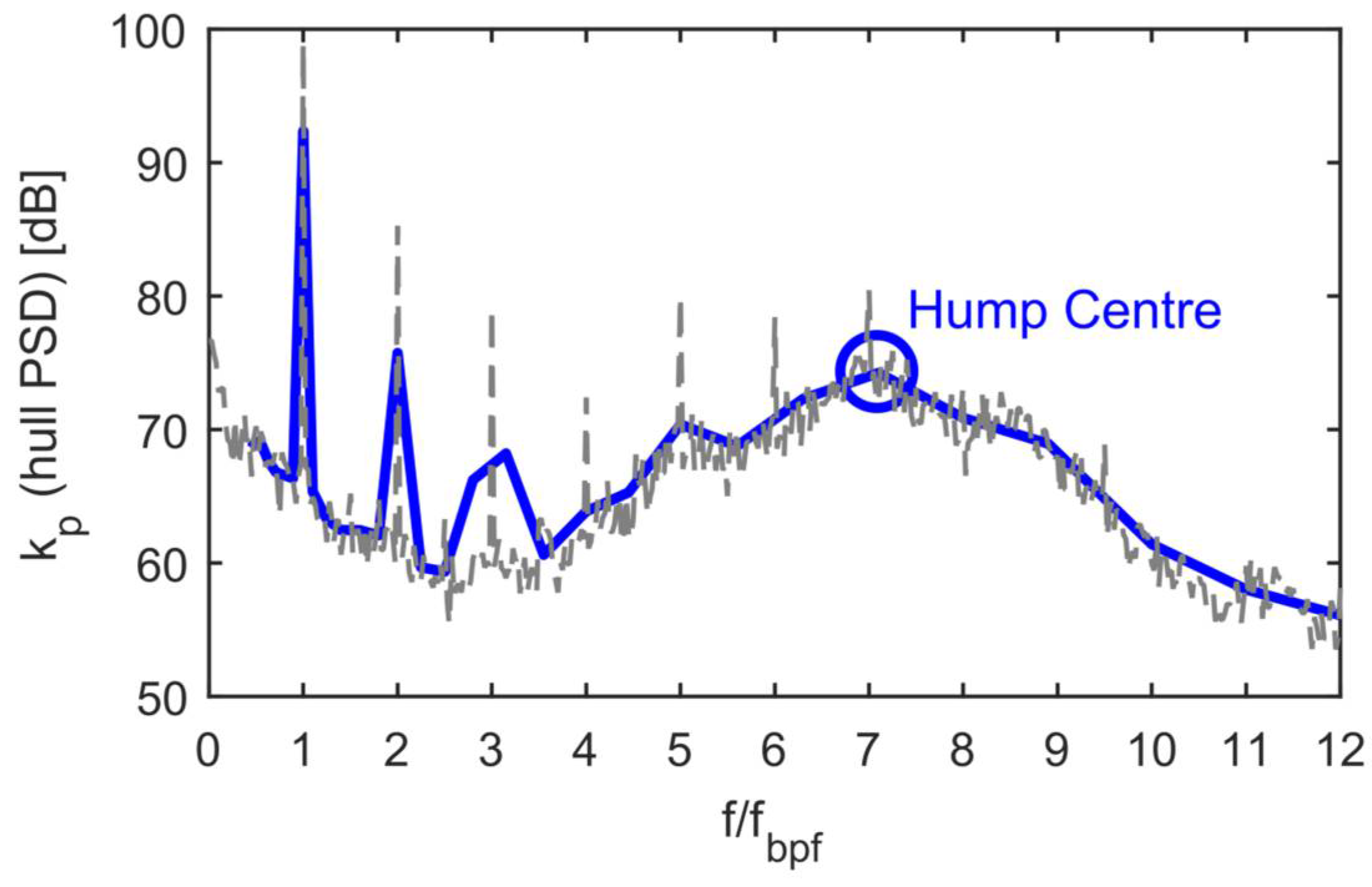
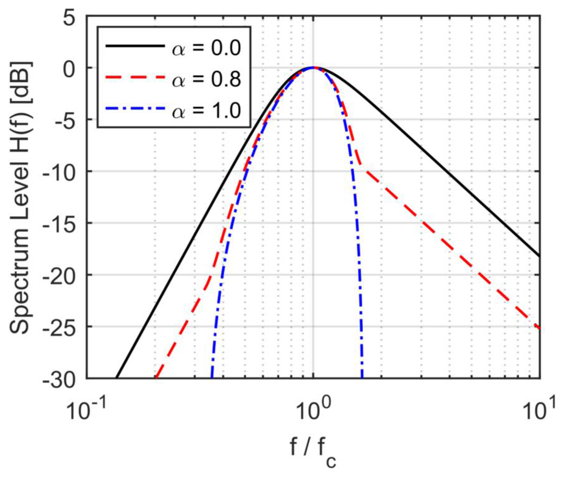
3. Shape of the Spectrum

3.1. Source Level

The shape of the spectrum of cavitation noise is described by e.g., [35,36,37]. The spectrum can be divided in a low-frequency part and a high-frequency part. The low-frequency part is characterized by a hump due to the overall growth, collapse and rebounds of the cavity. The high frequency part is related to the final phase of the collapse process during which velocities may approach or exceed the speed of sound, and compressibility effects become important. The collapse and rebounds of the smaller size bubbles generated by the collapse of the large scale cavity also contribute to the high frequency part.

In the present method, it is assumed that $f_c$ corresponds to a resonance frequency of the cavitating vortex. The related pressure signal can then be interpreted as a damped oscillatory signal, or, in a simplified way, as an oscillatory signal multiplied with a rectangular window. The Fourier transform of the latter is given by a sinc-function. Therefore, the shape of the spectrum, presented in decibel values, has been defined as

$$H_h\left(f\right)=20{\log }_{10}\left\{\mathrm{sinc}\left(\frac{f-f_c}{0.830\hspace{0.17em}\Delta f_{-6dB}}\right)\right\},$$

(15)

where $\Delta f_{-6dB}$ corresponds to the bandwidth of the hump where the pressure amplitude is half the maximum amplitude. A small value for $\Delta f_{-6dB}$ corresponds to a time trace with multiple rebounds (small damping) resulting in a narrow hump in the spectrum. A large value for $\Delta f_{-6dB}$ corresponds to a highly damped system resulting in a wide hump in the spectrum. Analysis of experimental data suggested that $\Delta f_{-6dB}$ is proportional to $f_c$, although the scatter is high.

The shape of the spectrum at much lower and higher frequencies than the centre frequency of the hump is modelled separately. The simple model used here consists of prescribed slopes at low and high frequency in a power density spectrum

$$H_s\left(f\right)=10{\log }_{10}\left\{\frac{2{\left(f/f_c\right)}^{{\alpha }_l}}{1+{\left(f/f_c\right)}^{{\alpha }_l-{\alpha }_h}}\right\},$$

(16)

in which ${\alpha }_h$ corresponds to the slope for high frequency, with typical value ${\alpha }_h=-2$, and ${\alpha }_l$ corresponds to the slope for low frequency, for which a value ${\alpha }_l=4$ is used as suggested in [35]. For different values of ${\alpha }_l$ and ${\alpha }_h$, the maximum value of $H_s$ is different from 0 dB, which needs to be corrected for.

The resulting spectrum is then taken as a weighted sum of powers of the two spectral functions

$$H\left(f\right)=10{\log }_{10}\left\{\alpha {10}^{H_h\left(f\right)/10}+\left(1-\alpha \right){10}^{H_s\left(f\right)/10}\right\},$$

(17)

where $\alpha$ is a user defined parameter. For practical applications, this parameter is computed from

$$\Delta L_{\alpha }=10{\log }_{10}\left(1-\alpha \right),$$

(18)

with $\Delta L_{\alpha }$ the difference in noise level between the maximum of the two-slope function and the maximum of the sinc function.

Examples of the shape of the spectrum for the source level are given in Figure 9 for three values of $\alpha$, where the curve for $\alpha =0.0$ corresponds to the spectrum for the two-slope function and the curve for $\alpha =1.0$ corresponds to the spectrum by the sinc function. In its current version, the default value is $\alpha =0.8$. For some cases, however, the default values do not give a good representation of the measured spectrum. It is remarked that the maximum absolute value of the argument of the sinc function has been limited to avoid the presence of ‘sidelobes’ in the spectrum.

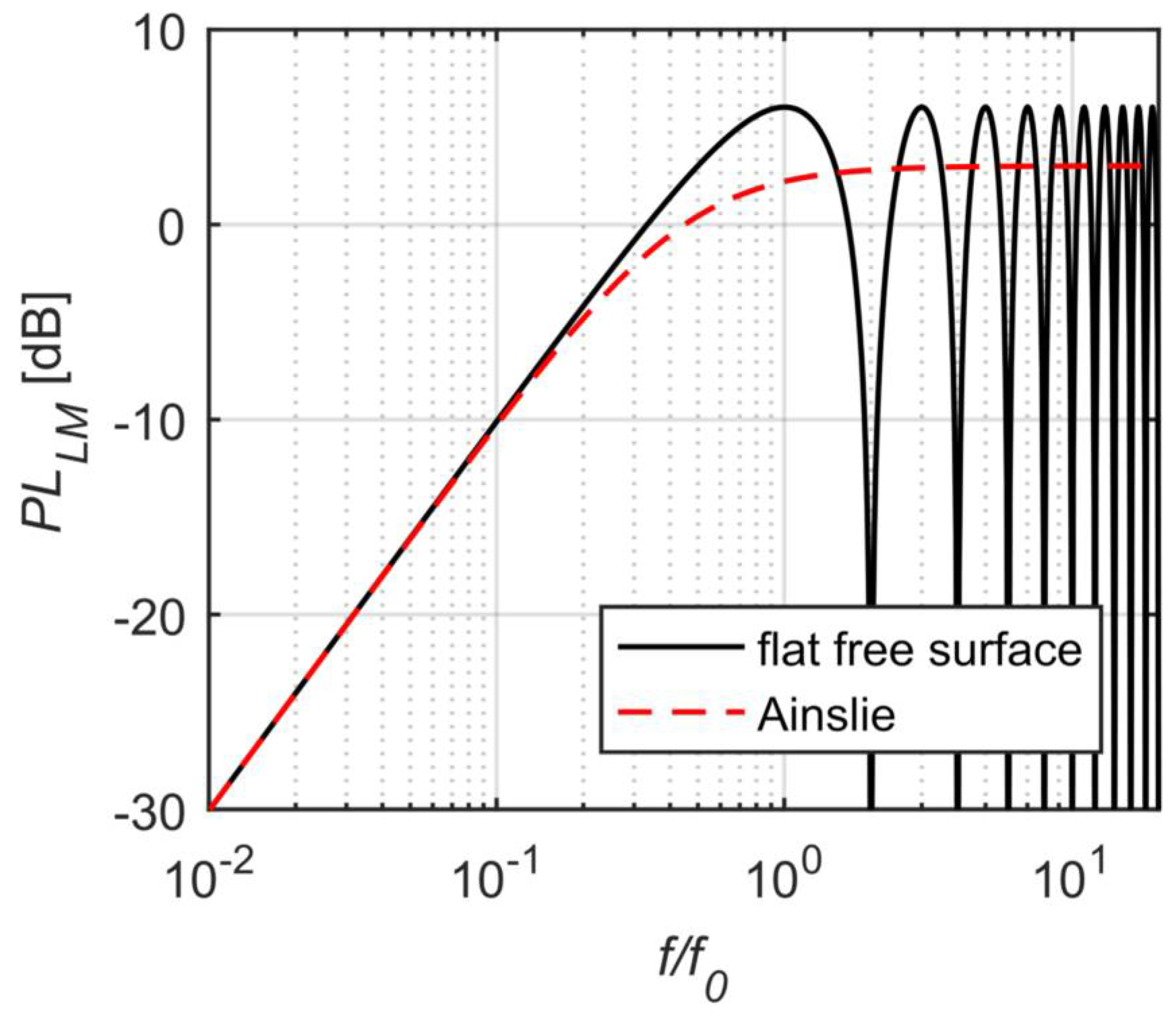
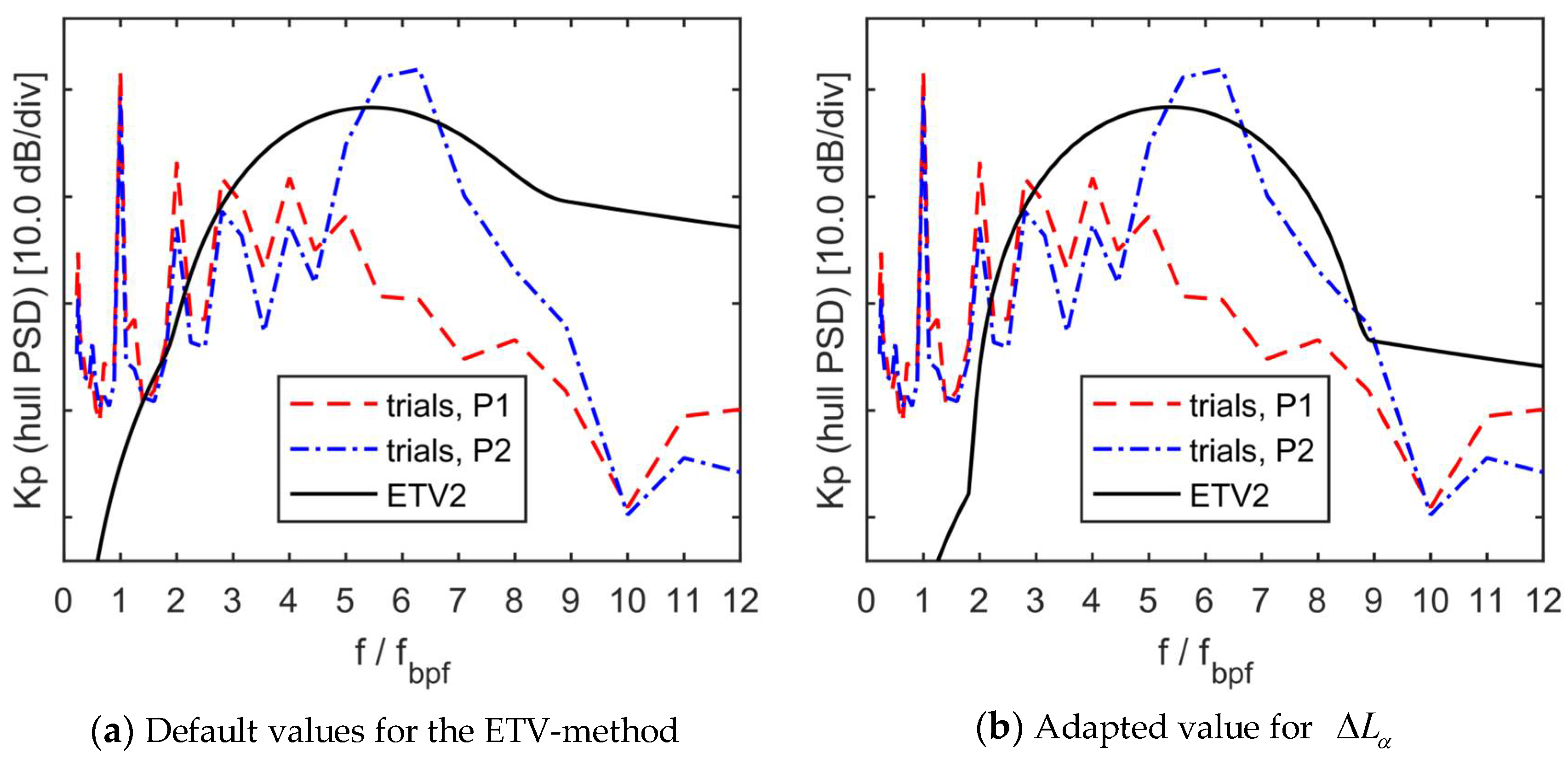
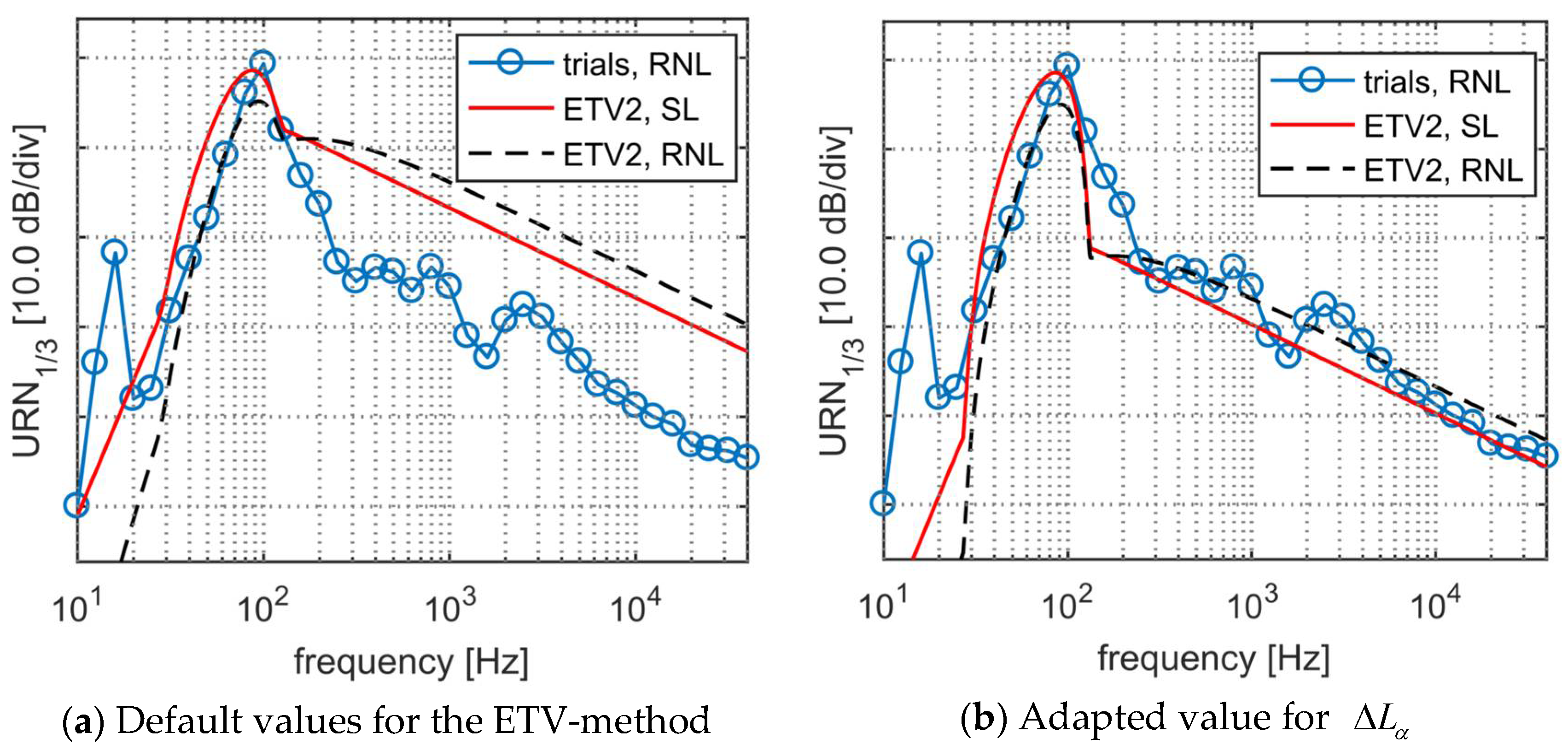
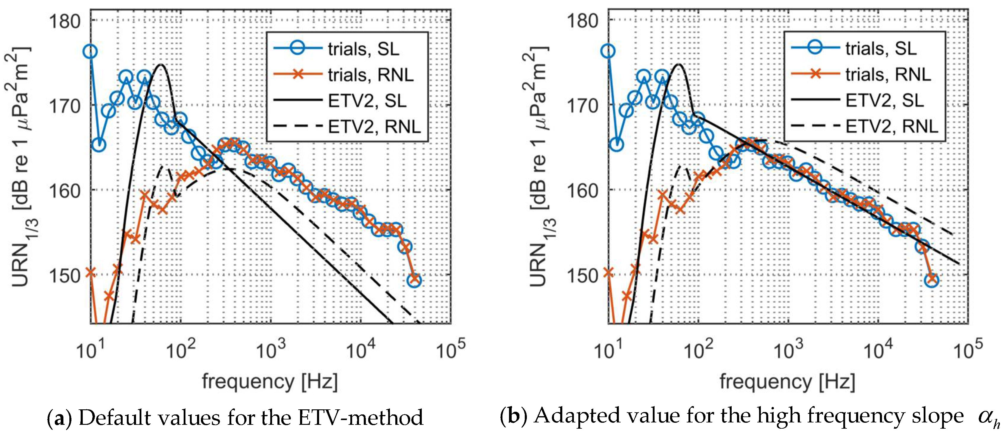
3.2. Hull-Pressure and URN Spectra

The hull-pressure spectrum is obtained from the source level spectrum by correcting for a solid boundary factor and for the propeller-hull clearance. The spectrum of the URN levels is obtained from the source level spectrum by correcting for the interference with the free surface (Lloyd’s mirror). A simple formula to correct for the propagation loss (PL) due to Lloyd’s mirror is given by Ainslie [38]

$$P{L}_{LM}=-10{\log }_{10}\left[\frac{1}{2}+\frac{1}{4k^2{d}_s^2{\sin }^2\theta }\right],$$

(19)

where $k$ corresponds to the acoustic wave number, $k=2\pi f/c$ with $c$ the speed of sound, $d_s$ to the submergence depth of the cavity collapse and $\theta$ to the hydrophone depression angle. The function is compared in Figure 10 to the theoretical formulation of the Lloyd’s mirror effect for a flat free surface [39]. The frequency in Figure 10 is made non-dimensional with the critical frequency $f_0$,

$$f_0=\frac{c}{4d_s\sin \theta }.$$

(20)

The interference patterns at frequencies above the critical frequency are usually not observed in ship noise data because of the presence of waves and bubbles near the free surface and the varying position between ship and hydrophone. For that reason, the Ainslie model assumes that, at high frequencies, the free surface leads to an uncorrelated image source.

The source level spectrum (SL) can now be defined as

$$SL\left(f\right)=L_{p,\max }+H\left(f\right)\hspace{1em}\left[\mathrm{dB},\hspace{0.17em}\hspace{0.17em}\mathrm{re}\hspace{0.17em}{1\mathsf{\mu }\mathrm{Pa}}^2{\mathrm{m}}^2/\mathrm{Hz}\right],$$

(21)

with $L_{p,\max }$ the maximum level of the hump of the power density spectrum, which is the dimensional value of $k_{p,\max }$. The spectrum of the underwater radiated noise level (RNL) is computed from the SL by correcting for Lloyd’s mirror

$$RNL\left(f\right)=SL\left(f\right)+P{L}_{LM}\left(f\right)\hspace{0.17em}\left[\mathrm{dB},\hspace{0.17em}\hspace{0.17em}\mathrm{re}\hspace{0.17em}{1\mathsf{\mu }\mathrm{Pa}}^2{\mathrm{m}}^2/\mathrm{Hz}\right].$$

(22)

The RNL levels, or URN levels in general, are often presented in one-third-octave band levels denoted by $RN{L}_{1/3}$ and $UR{N}_{1/3}$, respectively. The present model is referred to as ETV-2, the 2nd version of the Empirical Tip Vortex cavity model.

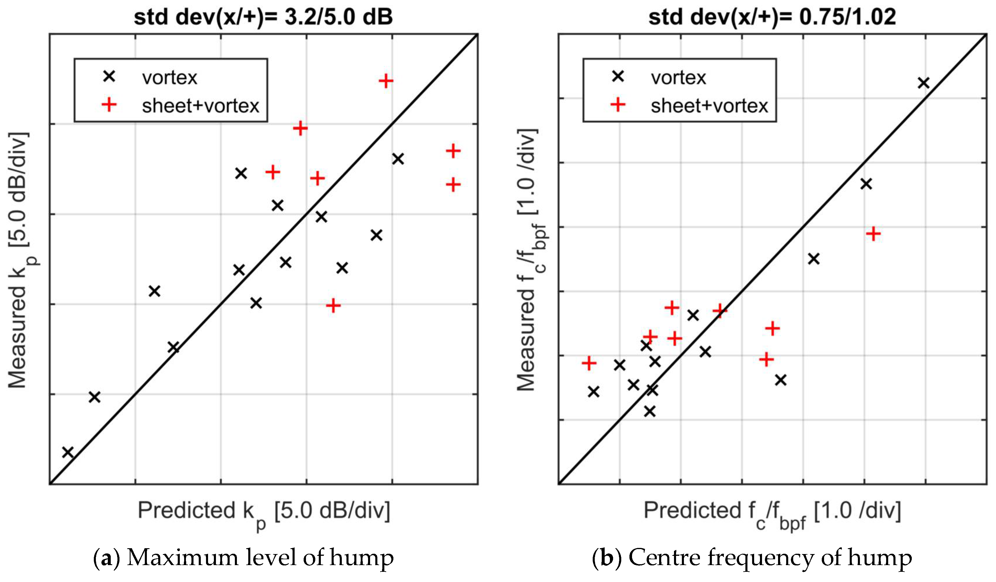
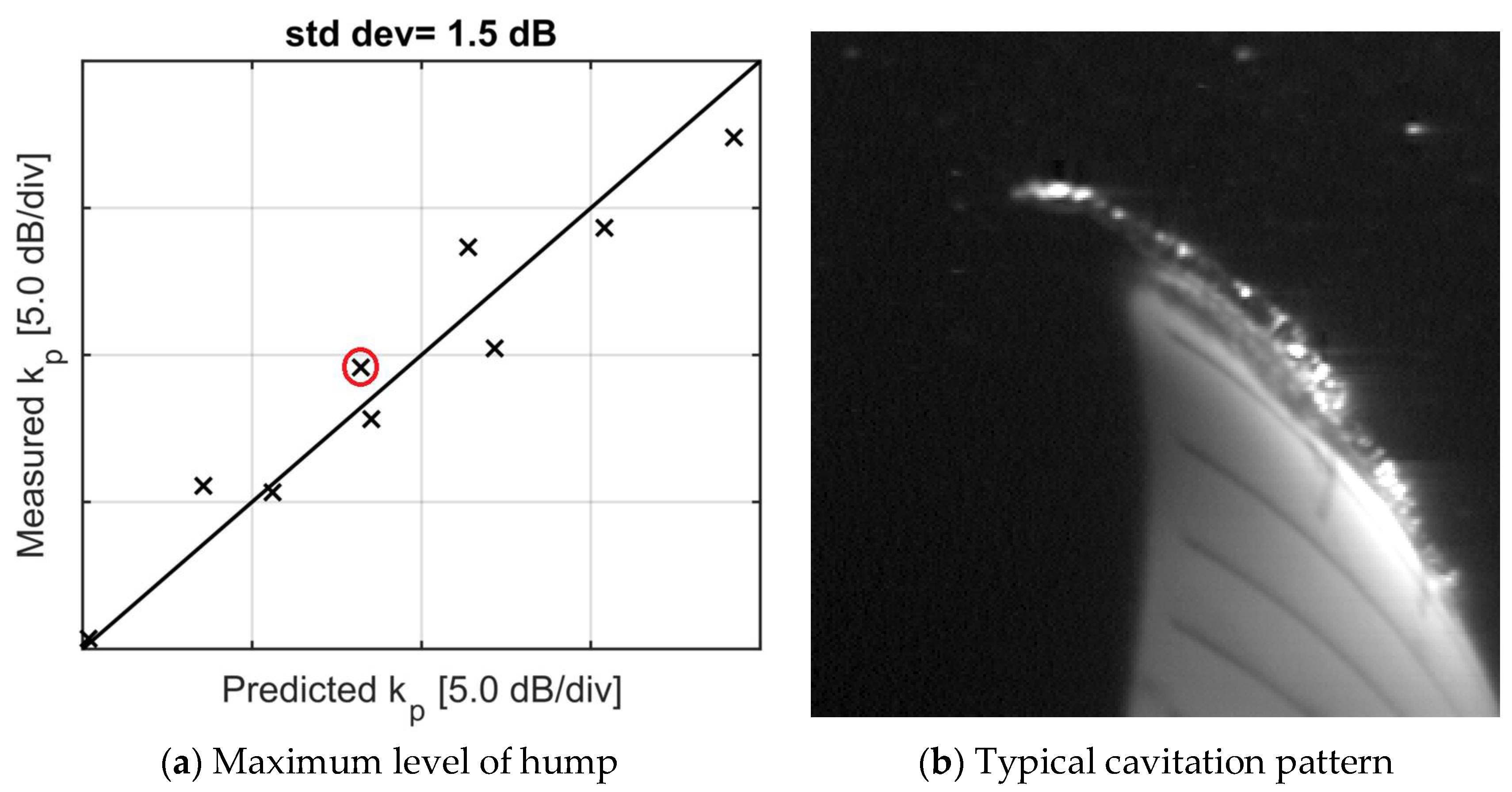
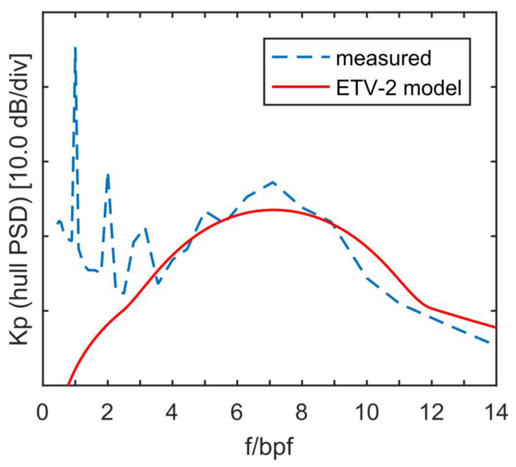
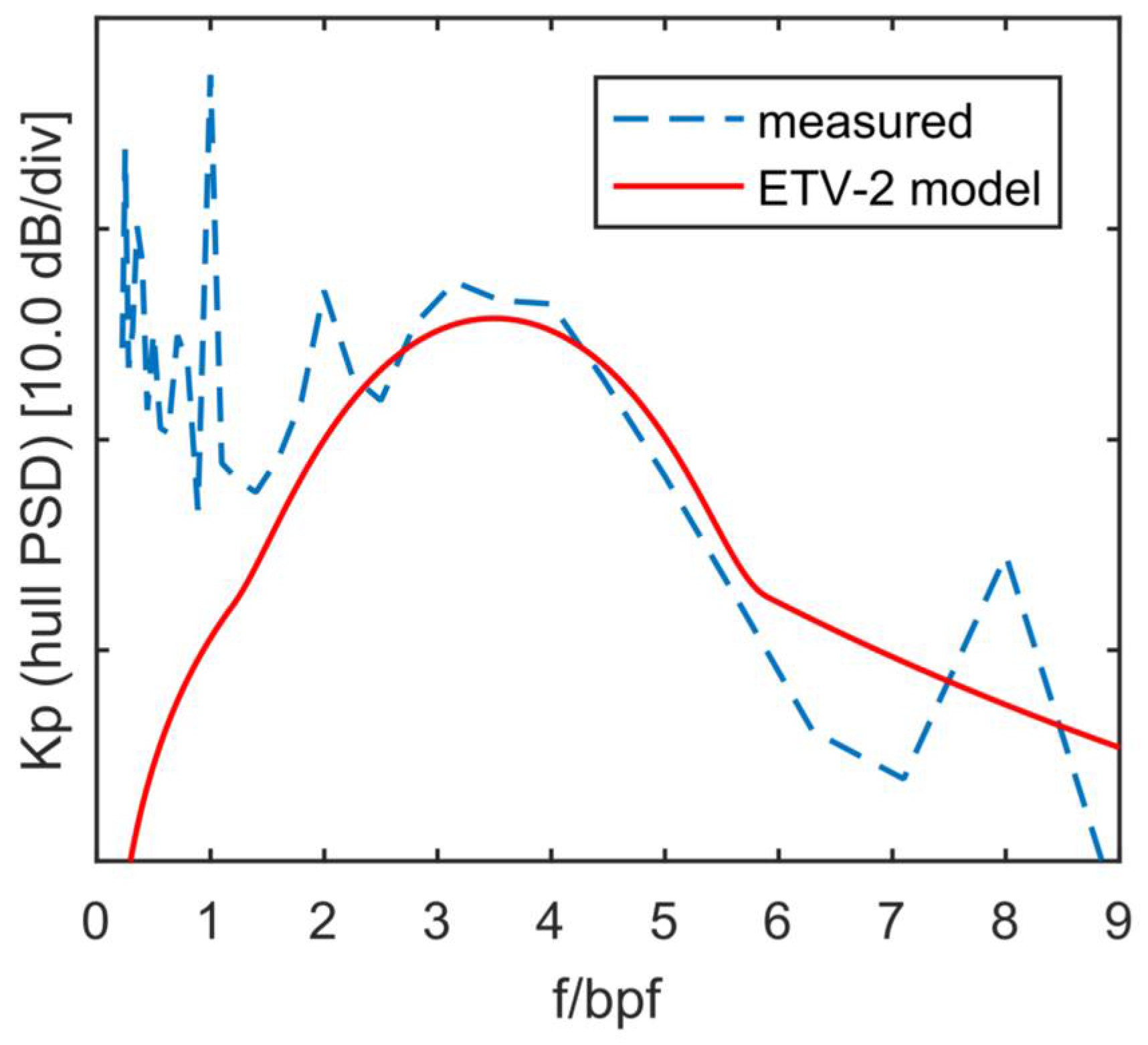
4. Comparison of Predicted and Measured Hull Pressures and URN

An example of the resulting spectrum of hull pressures predicted by the ETV model for the two-bladed research propeller is presented in Figure 11. Overall, the hump is well represented by the default spectral shape. The values of the empirical parameters for the maximum level and centre frequency were obtained from a dedicated fit to the test series for this propeller. The comparison between the resulting predicted and measured levels is given in Figure 8.

Examples of spectra for ship configurations used in the database are presented for model- and full scale in Figure 12 and Figure 13, respectively. Both cases are part of the vortex-cavitation group for which results are presented in Figure 7. The model- test results show some disturbance at the eighth harmonic of the blade passage frequency generated by the propeller drive train. However, this frequency is located at a much higher frequency than the broadband hump due to the cavitating tip vortex. Both figures are examples of cases that are well predicted by the model. As shown in Figure 7, there are also some cases for which the maximum level and centre frequency are predicted less accurately.

The model- and full-scale data are all made non-dimensional using Equation (8). Since no significant differences in the trend of the maximum level and centre frequency with scale could be discerned, it is concluded that Equation (8) can be used to scale the broadband pressure spectra from model scale to full scale. In fact, the equation can also be obtained by rewriting the formulation that is used to scale the (low-frequency) URN by cavitation as presented by e.g., Strasberg [40] and Bark [41].

The ETV-model has also been applied to predict the broadband hull-pressure levels on an 85 m combi freighter equipped with a single controllable pitch propeller. This ship was not in the database and, being a single screw vessel, it also does not resemble any ship in the data base. The sea trials for the ship, which included URN measurements in deep water, were performed by DAMEN, DNV-GL and MARIN and were financed by the CRS BROADBAND2 working group. The effective wake field for the PROCAL computation was obtained from a coupled RANS-BEM procedure [42,43]. Details of this data set are given in [44], which shows a comparison of the full-scale URN levels with predictions from model tests in the DWB. The cavitation pattern on the propeller was characterized by strong tip vortex cavitation. The values for the empirical constants derived using the complete database were used in the ETV method.

The comparison of broadband hull pressures as predicted by the ETV method and as measured during the sea trial at 10 knots is reasonable, as illustrated in Figure 14a. It is notable that the hump for this single screw ship is overpredicted by the ETV method. The URN of this vessel is dominated by a very pronounced hump that will be discussed later. This hump is not so obvious in the pressures measured by the centre transducer (P1) but can clearly be seen in the spectrum of the pressure sensor located closer to the collapse of the cavity (transducer P2).

In general, the results were considered to be quite acceptable for a range of pitch settings and shaft rotation rates as long as the cavitation was present on the back side of the blade. In its present form, the model was not capable of predicting the broadband pressure spectrum due to face side cavitation for a low pitch setting.

The model that was developed using data for hull pressures has also been applied to predict the URN due to propeller cavitation. The first test case considered for the prediction of URN is the single-screw combi freighter discussed above. The noise levels are presented in Figure 15a using the default values. The centre of the hump is well predicted in terms of level and frequency, but, at high frequencies, the predicted noise levels are approximately 10 dB too high. It is seen that the hump is very pronounced. The difference in noise levels between the hump and the high frequency region can easily be adjusted with the parameter $\Delta L_{\alpha }.$ Results for $\Delta L_{\alpha }=-20\hspace{0.17em}\hspace{0.17em}\mathrm{dB}$ are presented in Figure 15b. The default value for the slope of the spectrum at high frequencies is in good agreement with the sea-trial data. The hull-pressure prediction for this setting is also in better agreement with the experimental data (see Figure 14b).

The second data set analyzed is that of the (twin-screw) cruise vessel Statendam as reported by Kipple [45]. The length between perpendiculars is 182 m and the ship is driven by controllable pitch propellers. The URN measurements were performed in deep water. The measured SL are directly taken from [45] and the RNL are computed from the received noise levels at 500 yards as reported in [45]. All measured levels are converted to levels at 1 m distance assuming spherical spreading loss. The applied formulation in [45] to compute the source levels from the measured radiated noise levels is unknown, but the applied propagation loss is similar to Equation (19), except for high frequencies where the applied correction is 0 dB instead of 3 dB.

Results with default values are presented in Figure 16a. The maximum level is very well predicted, but the measured values in that frequency region are reported to be mainly due to machinery noise. At high frequencies, the agreement is not as good because the assumed slope of the spectrum is smaller than in the experiments. Adjustment of the high frequency slope to ${\alpha }_h=-1.6$ gives good agreement (see Figure 16b).

5. Discussion

The ETV-method has been developed to predict the broadband noise by propeller tip-vortex cavitation as present on propellers of twin screw vessels. Both model- and full-scale hull-pressure data were used for this purpose. The tip-vortex cavity is attached to the blade and might also be interpreted as an attached leading-edge vortex cavity that is directly connected to the tip vortex.

The majority of the test conditions were at or close to the design condition of the propeller. This restriction in variability of conditions was deemed necessary to avoid the influence of sheet cavitation on the measured hull-pressure data. Nevertheless, the cavitation observations showed that, for some of the cases, a combination of tip vortex cavitation and sheet cavitation was present. This sheet cavity detaches from the leading edge upstream of the blade tip. Due to the skew of the blade, the re-entrant jet flow at the cavity closure has a strong radial component, which is why it is sometimes called a side-entrant jet [46]. This side-entrant jet forms a cavity closure vortex [47] that is chordwise oriented in the tip region and that collapses when the blade leaves the wake peak. The propellers with such a cavitation pattern have been considered as a separate group.

The broadband noise levels for the propellers with such sheet and vortex cavitation was significantly higher than for propellers with vortex cavitation alone, requiring adjustment of the empirical parameter for the maximum level of the hump. Surprisingly, the adopted methodology still seems to apply to such a cavitation pattern indicating that the noise due to the collapse of the sheet-cavity closure vortex follows a similar trend as for the tip-vortex cavity. Another possibility is that the collapse of the closure vortex excites the cavitating tip-vortex and that the tip-vortex cavity is still responsible for the broadband hump. The standard deviation of the fit for this small group of propellers with sheet cavitation was higher than for the group with tip-vortex cavitation alone. Due to the two groups of tuning parameters, some information on the expected propeller cavitation pattern is required in the application of the method. This information can for instance be obtained from a sheet cavitation computation by the applied boundary element method. Such information can probably also be used to improve the fit for the group of propellers with sheet cavitation.

The test-cases used for the development of the method were all twin-screw vessels. Despite the limited variability of wake fields for these ships, the broadband hump was also well predicted for a single-screw vessel equipped with skewed propeller blades. This gives some confidence that the method is applicable to a wider range of wake fields. The most important limitation of the method is that it only describes the noise due to tip-vortex cavitation and, as discussed above, due to a sheet-cavity closure vortex in the tip region. The method is therefore mostly suited for the analysis of tip-unloaded (and skewed) propeller blades and is not expected to work for heavy-loaded propellers with extensive sheet cavitation.

The shape of the spectrum was not studied in much detail in the present study and requires further research. This not only holds for the higher frequency part of the spectrum, as shown by the URN prediction of the two test-cases shown, but also for the width of the broadband hump.

6. Conclusions

A semi-empirical method to predict broadband hull-pressure fluctuations and radiated noise by cavitating tip vortices on tip-unloaded propeller blades has been presented. The method makes use of results obtained by a boundary element method and can therefore very easily be used for propeller noise evaluation, for instance in a propeller design process. The principal parameter in the method is the vortex cavity size from which the maximum noise level and the centre frequency of the broadband hump was computed.

The standard deviation of the model fit was about 3 dB for the maximum level and 0.75 for the non-dimensional centre frequency, as long as no sheet cavitation was present on the propeller. When sheet cavitation was present in the tip area, the methodology could still be used, but the empirical parameter to predict the maximum of the hump had to be adjusted. The standard deviation of the model fit was higher than for the group with only tip-vortex cavitation.

The method was also applied to predict hull pressure fluctuations and URN of two vessels that were not used to develop the empirical relations. A good prediction was obtained for the broadband hump, but the high frequency region of the URN required adjustment of the empirical parameters that describe the spectral shape.

During the development and application of the method, a number of issues were identified that require further investigation. An important aspect is the contribution of sheet cavitation and the interaction between the sheet-cavity closure vortex and the tip-vortex cavity in the generation of the broadband hump. Another aspect is the overall shape of the spectrum, in particular the relation between the levels of the hump and the levels in the high-frequency part. Physical aspects that influence the shape of the hump and the slope of the high frequency noise also require further investigation.

References

1. Brubakk, E.; Smogeli, H. QE2 from turbine to diesel—Consequences for noise and vibration. In Proceedings of the IMAS Conference on the Design and Development of Passenger Ships, London, UK, 18–20 May 1988. [Google Scholar]
2. Carlton, J.S. Broadband cavitation excitation in ships. Ships Offshore Struct. 2015, 10, 302–307. [Google Scholar] [CrossRef]
3. Bosschers, J. Investigation of hull pressure fluctuations generated by cavitating vortices. In Proceedings of the First International Symposium on Marine Propulsors (SMP’09), Trondheim, Norway, 24–29 June 2009. [Google Scholar]
4. Pennings, P.C.; Bosschers, J.; Westerweel, J.; van Terwisga, T.J.C. Dynamics of isolated vortex cavitation. J. Fluid Mech. 2015, 778, 288–313. [Google Scholar] [CrossRef]
5. Bosschers, J. On the relation between tonal and broadband content of hull pressure spectra due to cavitating ship propellers. In Proceedings of the 9th International Conference on Cavitation (CAV2015), Lausanne, Switzerland, 6–10 December 2015. [Google Scholar]
6. Newman, M.; Abrahamsen, K. Measurement of underwater noise. In Proceedings of the Ship Noise and Vibration Conference, London, UK, 28–30 June 2007. [Google Scholar]
7. Foeth, E.J.; Bosschers, J. Localization and source-strength estimation of propeller cavitation noise using hull-mounted pressure transducers. In Proceedings of the 31st Symposium on Naval Hydrodynamics, Monterey, CA, USA, 11–16 September 2016. [Google Scholar]
8. Van Wijngaarden, H.C.J. Prediction of Propeller-Induced Hull-Pressure Fluctuations; Delft University of Technology: Delft, The Netherlands, 2011. [Google Scholar]
9. Johannsen, C.; van Wijngaarden, E.; Lücke, T.; Streckwall, H.; Bosschers, J. Investigation of hull pressure pulses, making use of two large scale cavitation test facilities. In Proceedings of the 8th International Symposium on Cavitation CAV2012, Singapore, 13–16 August 2012. [Google Scholar]
10. Bosschers, J.; Lafeber, F.H.; de Boer, J.; Bosman, R.; Bouvy, A. Underwater radiated noise measurements with a silent towing carriage in the Depressurized Wave Basin. In Proceedings of the 3rd International Conference on Advanced Measurement Technology for the maritime industry (AMT’13), Gdansk, Poland, 17–18 September 2013. [Google Scholar]
11. Tani, G.; Viviani, M.; Hallander, J.; Johansson, T.; Rizzuto, E. Propeller underwater radiated noise: A comparison between model scale measurements in two different facilities and full scale measurements. Appl. Ocean Res. 2016, 56, 48–66. [Google Scholar] [CrossRef]
12. Lafeber, F.H.; Bosschers, J. Validation of computational and experimental prediction methods for the underwater radiated noise of a small research vessel. In Proceedings of the PRADS2016, Copenhagen, Denmark, 4–8 September 2016. [Google Scholar]
13. Seol, H.; Suh, J.; Lee, S. Development of hybrid method for the prediction of underwater propeller noise. J. Sound Vib. 2005, 288, 345–360. [Google Scholar] [CrossRef]
14. Bosschers, J.; Vaz, G.; Starke, A.R.; van Wijngaarden, E. Computational analysis of propeller sheet cavitation and propeller-ship interaction. In Proceedings of the RINA MARINE CFD Conference, Southampton, UK, 26–27 March 2008. [Google Scholar]
15. Salvatore, F.; Testa, C.; Greco, L. Coupled hydrodynamics–Hydroacoustics BEM modelling of marine propellers operating in a Wakefield. In Proceedings of the First International Symposium on Marine Propulsors (SMP’09), Trondheim, Norway, 22–24 June 2009. [Google Scholar]
16. Matusiak, J. Pressure and Noise Induced by a Cavitating Marine Screw Propeller; Helsinki University of Technology: Espoo, Finland, 1992. [Google Scholar]
17. Brown, N.A. Thruster noise. In Proceedings of the Dynamic Positioning Conference of the Marine Technology Society, Houston, TX, USA, 12–13 October 1999. [Google Scholar]
18. Ligneul, P. Theory of tip vortex cavitation noise of a screw propeller operating in a wake. In Proceedings of the 17th Symposium on Naval Hydrodynamics, The Hague, The Netherlands, 13–14 June 1988. [Google Scholar]
19. Koronowicz, T.; Szantyr, J.A. Vortex cavitation as a source of high level acoustic pressure generated by ship propellers. Acta Acust. United Acust. 2006, 92, 175–177. [Google Scholar]
20. Berger, S.; Gosda, R.; Scharf, M.; Klose, R.; Greitsch, L.; Abdel-Maksoud, M. Efficient Numerical Investigation of Propeller Cavitation Phenomena causing Higher-Order Hull Pressure Fluctuations. In Proceedings of the 31st Symposium on Naval Hydrodynamics, Monterey, CA, USA, 11–16 September 2016. [Google Scholar]
21. Raestad, E. Tip Vortex Index—An Engineering Approach to Propeller Noise Prediction; Naval Architect; British Maritime Technology: London, UK, 1996; pp. 11–16. [Google Scholar]
22. Yamada, T.; Sato, K.; Kawakita, C.; Oshima, A. Study on prediction of underwater radiated noise from propeller tip vortex cavitation. In Proceedings of the 9th International Conference on Cavitation (CAV2015), Lausanne, Switzerland, 6–10 December 2015. [Google Scholar]
23. Vaz, G.; Bosschers, J. Modeling three dimensional sheet cavitation on marine propellers using a boundary element method. In Proceedings of the 6th International Symposium on Cavitation CAV2006, Wageningen, The Netherlands, 11–15 September 2006. [Google Scholar]
24. Bosschers, J.; Willemsen, C.; Peddle, A.; Rijpkema, D. Analysis of ducted propellers by combining potential flow and RANS methods. In Proceedings of the 4th International Symposium on Marine Propulsors (SMP’15), Austin, TX, USA, 31 May–4 June 2015. [Google Scholar]
25. Hommes, T.; Bosschers, J.; Hoeijmakers, H.W.M. Evaluation of the radial pressure distribution of vortex models and comparison with experimental data. In Proceedings of the 9th International Symposium on Cavitation (CAV2015), Lausanne, Switzerland, 6–10 December 2015. [Google Scholar]
26. Bosschers, J. An analytical and semi-empirical model for the viscous flow around a vortex cavity. Int. J. Multiph. Flow 2018, in press. [Google Scholar] [CrossRef]
27. Lamb, H. Hydrodynamics, 6th ed.; Cambridge University Press: Cambridge, UK, 1932. [Google Scholar]
28. Proctor, F.; Ahmad, N.; Switzer, G.; Duparcmeur, F.L. Three-phased wake vortex decay. In Proceedings of the AIAA 2010-7991: AIAA Atmospheric and Space Environments Conference, Toronto, ON, Canada, 2–5 August 2010. [Google Scholar]
29. Pennings, P.C.; Westerweel, J.; van Terwisga, T.J.C. Flow field measurement around vortex cavitation. Exp. Fluids 2015, 56, 1–13. [Google Scholar] [CrossRef]
30. Kuiper, G. Cavitation Inception on Ship Propeller Models. Ph.D. Thesis, Delft University of Technology, Delft, The Netherlands, 1981. [Google Scholar]
31. Jessup, S.D. An Experimental Investigation of Viscous Aspects of Propeller Blade Flow; The Catholic University of America: Washington, DC, USA, 1989. [Google Scholar]
32. McCormick, B.W. On cavitation produced by a vortex trailing from a lifting surface. J. Basic Eng. 1962, 84, 369–379. [Google Scholar] [CrossRef]
33. Shen, Y.T.; Gowing, S.; Jessup, S. Tip vortex cavitation inception scaling for high Reynolds number applications. J. Fluids Eng. 2009, 131, 071301. [Google Scholar] [CrossRef]
34. Hally, D. User ’s Guide for PIF-WAKE: The CRS PIF Wake Scaling Program for Single and Twin Screw Forms; Technical Report; DRDC Atlantic: Ottawa, ON, Canada, 2002. [Google Scholar]
35. Fitzpatrick, H.M.; Strasberg, M. Hydrodynamic sources of sound. In Proceedings of the First Symposium on Naval Hydrodynamics, Washington, DC, USA, 24–28 September 1956; pp. 241–280. [Google Scholar]
36. Lövik, A. Scaling of propeller cavitation noise. In Noise Sources in Ships; Nordforsk: Stockholm, Sweden, 1981. [Google Scholar]
37. Blake, W.K. Mechanics of Flow-Induced Sound and Vibration; Academic Press Inc.: Cambridge, MA, USA, 1986. [Google Scholar]
38. Ainslie, M. Principles of Sonar Performance; Springer: Berlin, Germany, 2010. [Google Scholar]
39. Clay, C.C.; Medwin, H. Acoustical Oceanography: Principles and Applications; John Wiley & Sons Ltd.: Hoboken, NJ, USA, 1977. [Google Scholar]
40. Strasberg, M. Propeller cavitation noise after 35 years of study. In Proceedings of the ASME Noise and Fluids Engineering, Altanta, GA, USA, 27 November–2 December 1977. [Google Scholar]
41. Bark, G. Prediction of Propeller Cavitation Noise From Model Tests and Its Comparison With Full Scale Data. J. Fluids Eng. 1985, 107, 112–120. [Google Scholar] [CrossRef]
42. Starke, B.; Bosschers, J. Analysis of scale effects in ship powering performance using a hybrid RANS-BEM approach. In Proceedings of the 26th Symposium on Naval Hydrodynamics, Gothenburg, Sweden, 26–31 August 2012. [Google Scholar]
43. Rijpkema, D.; Starke, B.; Bosschers, J. Numerical simulation of propeller-hull interaction and determination of the effective wake field using a hybrid RANS-BEM approach. In Proceedings of the 3rd International Symposium on Marine Propulsors (SMP’13), Launceston, Australia, 5–8 May 2013. [Google Scholar]
44. Lloyd, T.; Lafeber, F.H.; Bosschers, J. Investigation and validation of procedures for cavitation noise prediction from model-scale measurements. In Proceedings of the 32nd Symposium on Naval Hydrodynamics, Hamburg, Germany, 5–10 August 2018. [Google Scholar]
45. Kipple, B. Southeast Alaska Cruise Ship Underwater Acoustic Noise; NSWCCD-71-TR-2002/S74; Naval Surface Warfare Center—Detachment Bremerton: Washington, DC, USA, 2002. [Google Scholar]
46. Foeth, E.-J.; van Terwisga, T.; van Doorne, C. On the Collapse Structure of an Attached Cavity on a Three-Dimensional Hydrofoil. J. Fluids Eng. 2008, 130, 071303. [Google Scholar] [CrossRef]
47. Bark, G.; Bensow, R.E. Hydrodynamic mechanisms controlling cavitation erosion. In Proceedings of the 29th Symposium on Naval Hydrodynamics, Gothenburg, Sweden, 26–31 August 2012. [Google Scholar]
Figure 1. Flow chart of the Empirical Tip Vortex cavity (ETV) model for broadband hull pressure fluctuations and underwater radiated noise.
Jmse 06 00049 g001
Figure 2. Comparison between various vortex models. The reference values are taken from the values for the inviscid vortex at r = r v .
Jmse 06 00049 g002
Figure 3. Measured and fitted azimuthal velocity distribution and cavity size variation for a wing of elliptical planform at 7 deg angle of attack. Experiments by Pennings et al. [29].
Jmse 06 00049 g003
Figure 4. Measured and fitted cavity size variation for a propeller at two advance ratios. Experiments by Kuiper [30], Re n 1 = 1.38 × 10 6 , Re n 2 = 2.76 × 10 6 .
Jmse 06 00049 g004
Figure 5. Example of a non-dimensional hull pressure power density spectrum of a two-bladed research propeller. The solid line is the 1/6 octave band smoothened spectrum.
Jmse 06 00049 g005
Figure 6. Examples of cavitation patterns on the propellers used for the development of the method.
Jmse 06 00049 g006
Figure 7. Comparison between measured and predicted levels and frequency of the centre of the hump for the cases used in the development of the method.
Jmse 06 00049 g007
Figure 8. Comparison between measured and predicted maximum level of the hump for a two-bladed research propeller tested at various advance ratios and cavitation numbers. The cavitation pattern corresponding to the encircled symbol is shown on the right.
Jmse 06 00049 g008
Figure 9. Examples of the shape of the spectrum for different values of α .
Jmse 06 00049 g009
Figure 10. Propagation loss due to the Lloyd’s mirror effect.
Jmse 06 00049 g010
Figure 11. Example of the measured and predicted non-dimensional hull pressure spectrum for a two-bladed research propeller.
Jmse 06 00049 g011
Figure 12. Example of the measured and predicted non-dimensional hull pressure spectrum for a ship propeller of the database tested at model scale.
Jmse 06 00049 g012
Figure 13. Example of the measured and predicted non-dimensional hull pressure spectrum for a ship propeller of the database tested at full scale.
Jmse 06 00049 g013
Figure 14. Measured and predicted non-dimensional hull pressure spectrum for the combi-freighter at a ship speed of 10 knots. P1 corresponds to the centre transducer and P2 is located closer to the cavity collapse. Experimental data measured by DAMEN and MARIN.
Jmse 06 00049 g014
Figure 15. Measured and predicted radiated noise spectrum in one-third octave band levels for the combi-freighter at a ship speed of 10 knots. Experimental data by DNV-GL.
Jmse 06 00049 g015
Figure 16. Measured and predicted radiated noise spectrum in one-third octave band levels for the cruise vessel at a ship speed of 18 knots. Experimental data by Kipple [45].
Jmse 06 00049 g016