Fault-Tolerant Control for ROVs Using Control Reallocation and Power Isolation

Abstract

This paper describes a novel thruster fault-tolerant control system (FTC) for open-frame remotely operated vehicles (ROVs). The proposed FTC consists of two subsystems: a model-free thruster fault detection and isolation subsystem (FDI) and a fault accommodation subsystem (FA). The FDI subsystem employs fault detection units (FDUs), associated with each thruster, to monitor their state. The robust, reliable and adaptive FDUs use a model-free pattern recognition neural network (PRNN) to detect internal and external faulty states of the thrusters in real time. The FA subsystem combines information provided by the FDI subsystem with predefined, user-configurable actions to accommodate partial and total faults and to perform an appropriate control reallocation. Software-level actions include penalisation of faulty thrusters in solution of control allocation problem and reallocation of control energy among the operable thrusters. Hardware-level actions include power isolation of faulty thrusters (total faults only) such that the entire ROV power system is not compromised. The proposed FTC system is implemented as a LabVIEW virtual instrument (VI) and evaluated in virtual (simulated) and real-world environments. The proposed FTC module can be used for open frame ROVs with up to 12 thrusters: eight horizontal thrusters configured in two horizontal layers of four thrusters each, and four vertical thrusters configured in one vertical layer. Results from both environments show that the ROV control system, enhanced with the FDI and FA subsystems, is capable of maintaining full 6 DOF control of the ROV in the presence of up to 6 simultaneous total faults in the thrusters. With the FDI and FA subsystems in place the control energy distribution of the healthy thrusters is optimised so that the ROV can still operate in difficult conditions under fault scenarios.

1. Introduction

Over the past decades, the use of remotely operated vehicles (ROVs) has become more widespread. This is due to the reduction in costs driven by military and oil and gas research, making the technology available for other commercial and scientific purposes [1]. In more recent years ROVs have been employed for survey contracts and, with the push in the marine renewable energy (MRE) sector, ROVs will need to be capable of operating in more difficult environments to carry out close quarters inspections of the MRE devices and structures, thus reducing operational costs within the sector. The environment in which ROVs operate can be unpredictable, with the external parts of the system being subjected to seawater, changes in temperature, high pressures and interactions with solids drifting through the water column. These factors all contribute toward possibilities of thrusters becoming damaged or developing faults in their dynamic parts. In the past, it was common to abort a mission if a fault occurred in a thruster. Due to reduced weather windows at the sites of MRE converters [2], the expensive nature of ROV operations and the drive to reduce costs this method should be avoided, if possible. Fault-tolerant control system (FTC) within ROVs can be utilised to combat this. To accommodate faults and allow ROVs to manoeuvre in difficult environments they are usually designed so that they are over actuated. This increases the robustness of the system. Podder et al. utilised this configuration in a novel underwater vehicle approach for thruster force redistribution in the case of a fault [3]. Due to the particular advantages of FTC in ROV applications, many different techniques have been proposed:

Caccia et al. implemented thruster fault diagnosis by monitoring the motor current and revolutions per minute (RPM). If the monitored variables increased above a set threshold accommodation was performed by inhibiting the faulty thruster and by reconfiguring the distribution of the control actions cancelling the corresponding column in the thruster control matrix (TCM) [4].

Kim and Beale made use of Hotelling’s T2 statistic to diagnosis a fault in an underwater vehicle. They compared measured variable basis data used for training, with actual variable data and carried out statistical analysis. If the results of the statistical analysis were above a certain threshold then a fault was present. Further analysis determined if the fault occurred in the stern plane (vertical) or rudder (horizontal). The system was designed so that the controller was reconfigurable, meaning that the type of fault in the system determined the type of controller to be utilised. Their tests were carried out in simulations and found that noise can increase fault detection times [5].

Montazeri et al. proposed fault diagnosis in the steering system of an autonomous underwater vehicle (AUV) through the use of two different neural network systems (multi-layer perceptron (MLP) and Adaline). This method, validated using simulations, was capable of detecting both partial and full faults. Results found that the speed of the MLP fault detection was lower than the Adaline method due to its larger complexity [6]. Zhu et al. utilised a neural network to increase the performance of on-line fault detection in thrusters on an open-frame ROV and provide appropriate control reallocation. This approach was tested in simulations but only total faults of the thruster were taken into consideration, which was different from the simulated fault situation of the thrusters [7].

A combination of tools was employed by Hai et al. for a fault-tolerable control scheme for an open-frame ROV. The methods combined were a petri network and a recurrent fuzzy neural network (PRFNN). This approach combines the advantages of low level learning, high level reasoning and reduced calculations. Simulation and experiments proved that the ROV FTC could accurately detect partial and full faults and accommodate this in the control [8].

Another previous approach was to integrate self-organizing maps and fuzzy logic clustering to achieve fault diagnosis. Upon diagnosing the fault a novel weighted pseudo-inverse scheme compensated in the control [9].

Liu and Zhu conducted thruster external fault diagnosis on an ROV by comparing expected heading values with actual heading values for a given control voltage and referencing it back to a fault code table [10]. Akmal et al. developed a fuzzy based thruster fault diagnosis and accommodation system, which monitored voltage and current, and compared it to pre-measured values. The values of the resulting residuals were then used to compare to a fuzzy fault code table, assigning PWM control constraints to the thrusters, depending on their state. This simple approach was successful but was unable to distinguish if there was an internal or external fault [11].

The FTC system for an ROV, proposed in [12], used a modified version of the Moore-Penrose pseudo inverse to redistribute the control effort to healthy thrusters if a fault occurs.

In the literature the majority of the fault-tolerant control methods proposed for underwater vehicles have been integrated and evaluated in a simulated environment. As a first step for evaluation this approach is beneficial but, when practical and affordable, real-world trials should be conducted to evaluate the system in the environment in which it is expected to operate. Real-world trials have been conducted in some cases to evaluate the FTC of the ROV [4,12], generating more accurate results.

This paper presents an active fault-tolerant control system for an ROV using a combination of thruster fault detection and isolation, faulty thruster power isolation and fault accommodation in the control of the ROV. The word “active” means that the method is based on active monitoring of relevant signals from the thrusters (currents, shaft speeds, applied voltages and temperatures of windings). For thrusters that cannot provide these signals, the authors are currently working on novel “passive” method for fault detection and isolation. It is expected to publish the main features of the “passive” method and comparison table of both methods in Spring 2018.

Most underwater vehicle fault detection schemes are model-based, and concern the dynamic relationship between actuators and vehicle behaviour or the specific input-output thruster dynamics [13]. The proposed thruster fault detection and isolation (FDI) approach is a model-free scheme based on a pattern recognition neural network, trained with simulated and real-world data. New features of the proposed FTC includes separation of the virtual control space into vertical and horizontal thruster subspaces (planes) and real-world implementation in the real-time ROV control system for various thruster configurations. The thruster FA subsystem receives thruster state data from the FDI and, in the case of a fault, reallocates thruster forces by reducing the saturation bounds of the faulty thruster (software-level action A). At the same time, in case of total faults, the thruster power is switched off (hardware-level action B), in order to prevent a threat to full power system and reduce the risk of damage to other ROV components.

The proposed FTC system has been successfully tested in a virtual environment (using a real time ROV simulator, created at CRIS, in the University of Limerick (UL)) and a real world environment (using VM5 thrusters from VideoRay in Pottstown, PA, USA) in a test tank at UL. The proposed FTC system is part of the OceanRINGS+ ROV smart control system, currently under development at CRIS, UL.

The paper outline is provided as follows. In Section 2 background information is provided, including links with other research projects and a short description of Inspection ROV (IROV). The architecture of the FTC, including description and implementation of the FDI & FA subsystems, is described in Section 3. Section 4 presents the testing and evaluation results of the proposed FTC in real-world and virtual (simulated) environments. Finally, concluding remarks and directions for future work are provided in Section 5.

2. Background

2.1. OceanRINGS⁺

OceanRINGS is an Internet/Ethernet-enabled ROV control system, based on robust control algorithms, deterministic network-oriented hardware and flexible, 3-layer software architecture [14]. ROV LATIS is a prototype platform developed at UL to test and validate OceanRINGS [15]. System validation and technology demonstration has been performed over the last eight years through a series of test trials with different support vessels. Operations include subsea cable inspection/survey, wave energy farm cable to shore routing, shipwreck survey, ROV-ship synchronisation and oil spill/HNS incident response.

Currently, researchers at UL are developing the next generation of the ROV control system (OceanRINGS⁺, the extended version of OceanRINGS). The highly adaptive 3-layer software architecture of OceanRINGS⁺ includes fault-tolerant control allocation algorithms in the bottom layer, transparent interface between an ROV and supporting platforms (surface platforms, surface/subsea garages and/or supporting vessels) in the middle layer and assistive tools for mission execution/monitoring/supervision in the top layer. Software modules have been developed for advanced control modes, such as auto compensation of ocean currents based on ROV absolute motion, robust speed/course controller with independent heading control, semi and full auto pilot capabilities, auto-tuning procedure for low-level controllers, ROV high precision dynamic position & motion control in absolute earth-fixed frame, or relative to target or support platform/vessel. This paper is focused on the description of the FTC, the module at the bottom layer of the full OceanRINGS⁺ control architecture.

2.2. Inspection-Class Remotely Operated Vehicle (I-ROV)

As part of the ongoing MaREI research project “Smart Inspection ROVs for Use in Challenging Conditions”, researchers at the Centre for Robotics & Intelligent Systems (CRIS), University of Limerick have designed and developed a reconfigurable, inspection-class ROV (I-ROV) in the period of 2014–2018, aimed to perform periodic and post storm inspection of offshore MRE converters, moorings and foundations, reducing the need for commercial divers to be employed in this difficult and potentially dangerous environment. The I-ROV (Figure 1) is a reconfigurable system with the option to utilise two types of thrusters in different configurations.

The reconfigurable propulsion system of I-ROV includes two thruster configurations (

Table 1. Thruster configurations.

Configuration 1: 8 × M5 Thrusters	Configuration 2: 12 × T200 Thrusters
Horizontal Layer: HT1, HT2, HT3, HT4	Horizontal Layer (L0): HT1, HT2, HT3, HT4
	Horizontal Layer (L1): HT1, HT2, HT3, HT4
Vertical Layer: VT1, VT2, VT3, VT4	Vertical Layer: VT1, VT2, VT3, VT4

):

• Configuration 1: Eight VideoRay M5 thrusters configured in two layers: Horizontal Layer with four thrusters and Vertical Layer with four thrusters. These thrusters provide active monitoring of relevant signals from thrusters (currents, shaft speeds, applied voltages and temperatures of windings).
• Configuration 2: Twelve Blue Robotics T200 thrusters configured in three layers: Horizontal Layers L0 and L1 with four thrusters each and Vertical Layer with four thrusters. These thrusters cannot provide monitoring of relevant signals and the passive FTC system for this class of thruster is under development.

It should be emphasized that the OceanRINGS⁺ control architecture has been designed to be generic, i.e., not limited to exclusive use by IROV, but any ROV with standard physical layout of thrusters. Although testing and validation of proposed FTC is performed with IROV configured as Configuration 1, the active FTC proposed in this paper and implemented as part of OceanRINGS⁺ is applicable to open-frame ROVs with a maximum of 12 thrusters subject to the constraint that each thruster can provide measurement of relevant signals (currents, shaft speeds, applied voltages and temperatures of windings). The FDI subsystem detects faults in thrusters regardless of their physical layout. However, for successful fault accommodation, the physical layout of thrusters plays an important role.

3. Fault-Tolerant Control (FTC) System

3.1. FTC Architecture

The overall functional architecture of the proposed FTC system is shown in Figure 2. The description of the architecture is provided in a hierarchical manner, such that the general description and the main idea are introduced first, while more details about individual components can be found in the following subsections. This architecture is an extension of the control architecture proposed in [16].

In contrast to the Fault Diagnosis and Accommodation System (FDAS), proposed in [17] and implemented in the original version of OceanRINGS, there are a number of new features in the FTC architecture shown in Figure 2 and implemented in OceanRINGS⁺. Firstly, there is a clear separation between horizontal and vertical thrusters using decomposition of motion into horizontal and vertical subspaces (planes). Secondly, there is provision for two layers of horizontal thrusters and one layer of vertical thrusters. Thirdly, the Fault Detection Units utilize a pattern recognition neural network for real-time fault detection instead of self-organising maps.

The virtual control input τ for the control allocation is a normalised vector of forces and moments: $\tau ={\left[\begin{array}{cccccc}{\tau }_X& {\tau }_Y& {\tau }_Z& {\tau }_K& {\tau }_M& {\tau }_N\end{array}\right]}^T$, where ${\tau }_X$ is surge force, ${\tau }_Y$ is sway force, ${\tau }_Z$ is heave force, ${\tau }_K$ is roll moment, ${\tau }_M$ is pitch moment, and ${\tau }_N$ is yaw moment. Decomposition of this vector into the horizontal and vertical planes is presented in

Table 2. Decomposition into Horizontal and Vertical Subspaces (Planes).

Virtual Control Input	Horizontal Plane ${\mathit{\tau }}_{\mathit{H}\mathit{T}}$		Vertical Plane ${\mathit{\tau }}_{\mathit{V}\mathit{T}}$
$\tau =\left[\begin{array}{c}{\tau }_X\\ {\tau }_Y\\ {\tau }_Z\\ {\tau }_K\\ {\tau }_M\\ {\tau }_N\end{array}\right]$	${\tau }_{HT}=\left[\begin{array}{c}{\tau }_X\\ {\tau }_Y\\ {\tau }_N\end{array}\right]$	${\tau }_X$—Surge Force	${\tau }_{VT}=\left[\begin{array}{c}{\tau }_Z\\ {\tau }_K\\ {\tau }_M\end{array}\right]$	${\tau }_Z$—Heave Force
		${\tau }_Y$—Sway Force		${\tau }_K$—Roll Moment
		${\tau }_N$—Yaw Moment		${\tau }_M$—Pitch Moment

.

The Control Clusters (Figure 2 and Table 2) are links between the FTC module in the bottom layer and upper layers in control architecture. The HT Control Cluster consists of two subclusters: Virtual Joystick (to mimic direct surge & sway forces and yaw moment generated by human or virtual pilot) and a set of settings for Low-Level Controllers (set points for surge speed $u_d$ (m/s), sway speed $v_d$ (m/s) and heading $Y_d$ (°), feed-forward inputs and on/off switches to enable/disable individual controllers). The VT Control Cluster has two subclusters: Virtual Joystick (to mimic direct heave force and roll & pitch moments generated by human or virtual pilot) and a set of settings for Low-Level Controllers (set points for depth/altitude $z_d$ (m), roll $R_d$ (°) and pitch $P_d$ (°), feed-forward inputs and on/off switches to enable/disable individual controllers). Inside the Synthesis module the LLC Settings subclusters are used as one of the inputs to the LLC loops (the other inputs are navigation data and parameters of controllers). There is a single controller for each degree of freedom (DOF). Surge and Sway controllers are velocity controllers, while Heave, Roll, Pitch & Yaw are position controllers. Further information about the internal structure of LLC loops can be found in [9]. Individual outputs of LLC loops are bundled into vectors ${\tau }_{LLC}$. The final outputs of the Synthesis module are vectors ${\tau }_{HT}$ and ${\tau }_{VT}$, obtained by summation and normalisation of corresponding vectors ${\tau }_{VJ}$ and ${\tau }_{LLC}$ for each subspace, respectively.

Each layer of horizontal thrusters has its own FDI, FA and Control Allocator module. It should be emphasized that both layers of horizontal thrusters are independent from each other, i.e., they can have a different physical layout and number of thrusters. In the Horizontal Plane, both layers have the same input (vector τ_HT), which is the output of HT Synthesis module.

3.2. Fault Detection and Isolation (FDI) Subsystem

3.2.1. Fault Classification

Thrusters are liable to different fault types during the underwater mission e.g., propellers can be jammed, broken or lost, water can penetrate inside the thruster enclosure, communication between the thruster and the master node can be lost, applied voltage or temperature of the winding can exceed the threshold, etc. Some of these faults (partial faults) are not critical and the thruster is able to continue operation in the presence of a fault with the restricted usage, i.e., reduced maximum velocity. In other cases (total faults—failures) the thruster must be switched off and the mission has to be continued with remaining operable thrusters. Thruster faults are classified into two main classes:

• Internal faults (e.g., temperature of the windings is out of range, drop in bus voltage etc.),
• External faults (e.g., lightly jammed, jammed, heavily jammed, lost or broken propeller).

3.2.2. Fault Code Table

Relationships between thruster states, fault types and remedial actions are stored in the thruster fault code table (

Table 3. Thruster Fault Code Table.

Thruster State	Class	Type	Action A: Saturation Bounds	Action B: Thruster Power
Invalid	-	-	1.00	ON
Healthy	-	-	1.00	ON
Lightly Jammed	External	Partial	0.75	ON
Jammed	External	Partial	0.25	ON
Heavily Jammed	External	Total	0.00	OFF
Broken Propeller	External	Total	0.00	OFF
Unknown	External	Total	0.00	OFF
Voltage outside threshold	Internal	Total	0.00	OFF
Temp. outside threshold	Internal	Total	0.00	OFF

). It must be emphasized, at this point, that this fault code table is just a suggestion, intended to reveal the main ideas of the proposed FTC system. New states (rows) can be added, and the existing relationships can be changed, in order to accommodate specific requirements and available thruster data. For example, other faults like thruster shaft misalignment or damaged bearings can cause excessive vibration, increased temperature and, in worst case scenarios, cause flooding through broken shaft or damaged enclosure [18].

3.3.3. Fault Detection Unit (FDU)

It is assumed that each thruster is driven by a Thruster Control Unit (TCU), with integrated power amplifiers and a microcontroller (Figure 3). The input to the TCU is desired shaft speed $n_d$ (%). The outputs are current $I$ (A), shaft speed $n$ (rpm), bus voltage $V$ (V) and temperature $T$ (°C) of windings. The outputs of each thruster are sent to the associated FDI module in real-time. The FDI module utilises the Fault Detection Units (FDUs) to monitor the state of the thrusters. The FDU is a software module associated with the thruster, able to detect internal faults and external faults. The output of the FDU is a fault state vector $f_i$. Connections between the FDU and the TCU for an arbitrary thruster $T_i$ are indicated in Figure 3.

Signals for detection of internal faults are already available in existing TCUs for VideoRay thrusters M5. In particular, the communication protocol for the M5 provides monitoring of the winding temperature T (°C) and bus voltage V (V) of each thruster. In order to build a universal FDU, able to detect both internal and external faults, it is necessary to augment the existing internal protection with a software module for fast and reliable detection of external faults.

For detection of external faults available signals are desired: shaft speed $n_d$ (%), actual shaft speed $n$ (rpm) and current consumption $I$ (A) of the thruster. By monitoring $n$ and $I$, together with desired shaft speed $n_d$, obtained as the output of the Control Allocation, the FDU is designed to detect, isolate and categorise external thruster faults using Pattern Recognition Neural Network (PRNN).

Finally, the universal FDU integrates both parts (internal and external) into one unit, which is able to detect both internal and external faults (Figure 3). Integration includes a priority scheme, where total faults have higher priority than partial faults. The fault state vector $f_i$, the output of the FDU, is the code of the fault.

3.3.4. Implementation

Implementation involves two phases: off-line training and on-line fault detection.

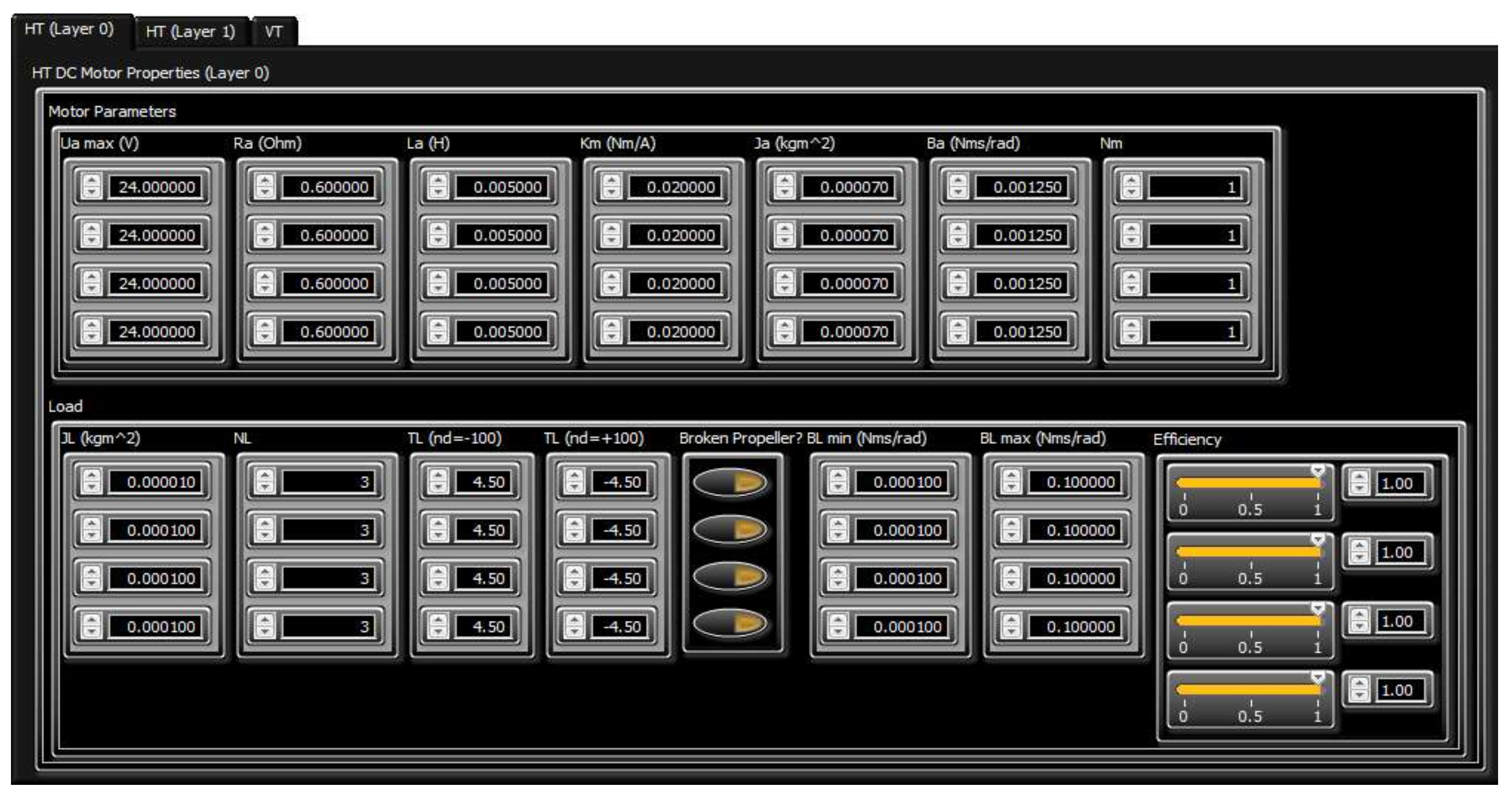
Off-Line Training Phase

The first stage in the training phase is acquisition of training data. In the virtual environment, thruster faults are simulated by varying properties of the thruster dynamic model (load, friction, etc.) inside the propulsion subsystem of the ROV dynamics simulator. In the real-world environment, various jammed propeller faults are simulated such that the objects of different sizes, shapes and weights were attached to the blades, while a broken propeller was simulated with all blades removed from the shaft. Further details about acquisition of training data in real-world environment is given in the following. A normal state and four different fault cases were considered (lightly jammed, jammed, heavily jammed and broken (lost) propeller). A test rig has been set up and thruster mounted in a test tank in the University of Limerick. To mimic the jammed thruster states various objects (“blockages”) have been attached to the thruster propeller during tests. The thruster test setup and “blockages” are shown in Figure 4. Each “blockage” reduces efficiency of the thruster due to increased load on the shaft and reduced flow of the water through the duct.

The relationship between the thruster states and setup for real-world data acquisition is given in

Table 4. Thruster states & setup for real-world data acquisition.

Thruster State	Setup
Healthy	No blockage
Lightly Jammed	Blockage (30% area)
Jammed	Blockage (60% area)
Heavily Jammed	Blockage (90% area)
Broken Propeller	Propeller detached

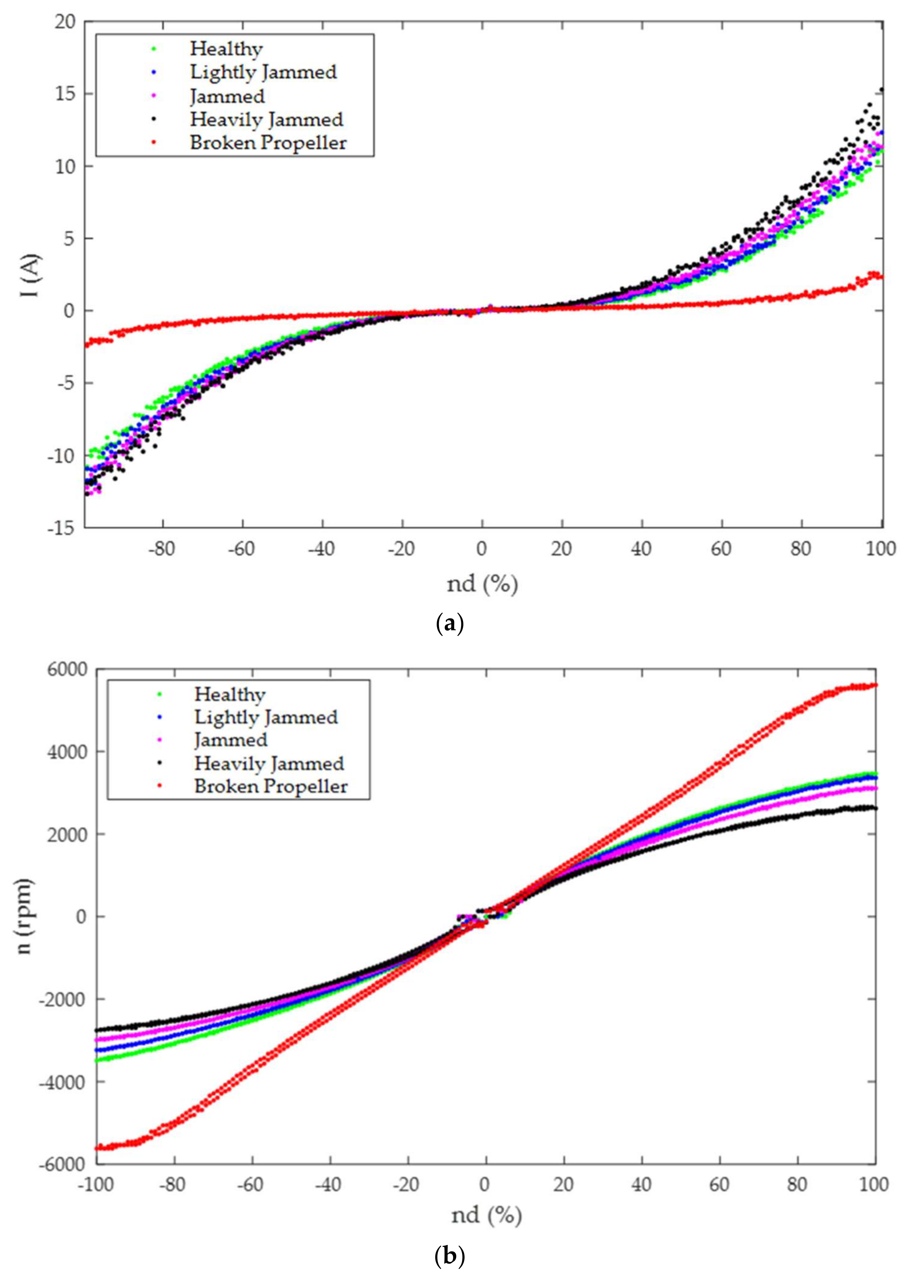
. For each state in Table 4, the thruster was actuated with a saw-like command signal $n_d$ (%) with the following pattern: 0% » MAX% » 0% » −MAX% » 0%, with a step size 1%. The total duration of signal was 20 s, sampling period 50 ms and max. value MAX = 100%. In each iteration the desired shaft speed $n_d$ (%), actual shaft speed $n$ (rpm) and current consumption $I$ (A) have been logged. The real-world raw data acquired for each thruster state are presented in Figure 5.

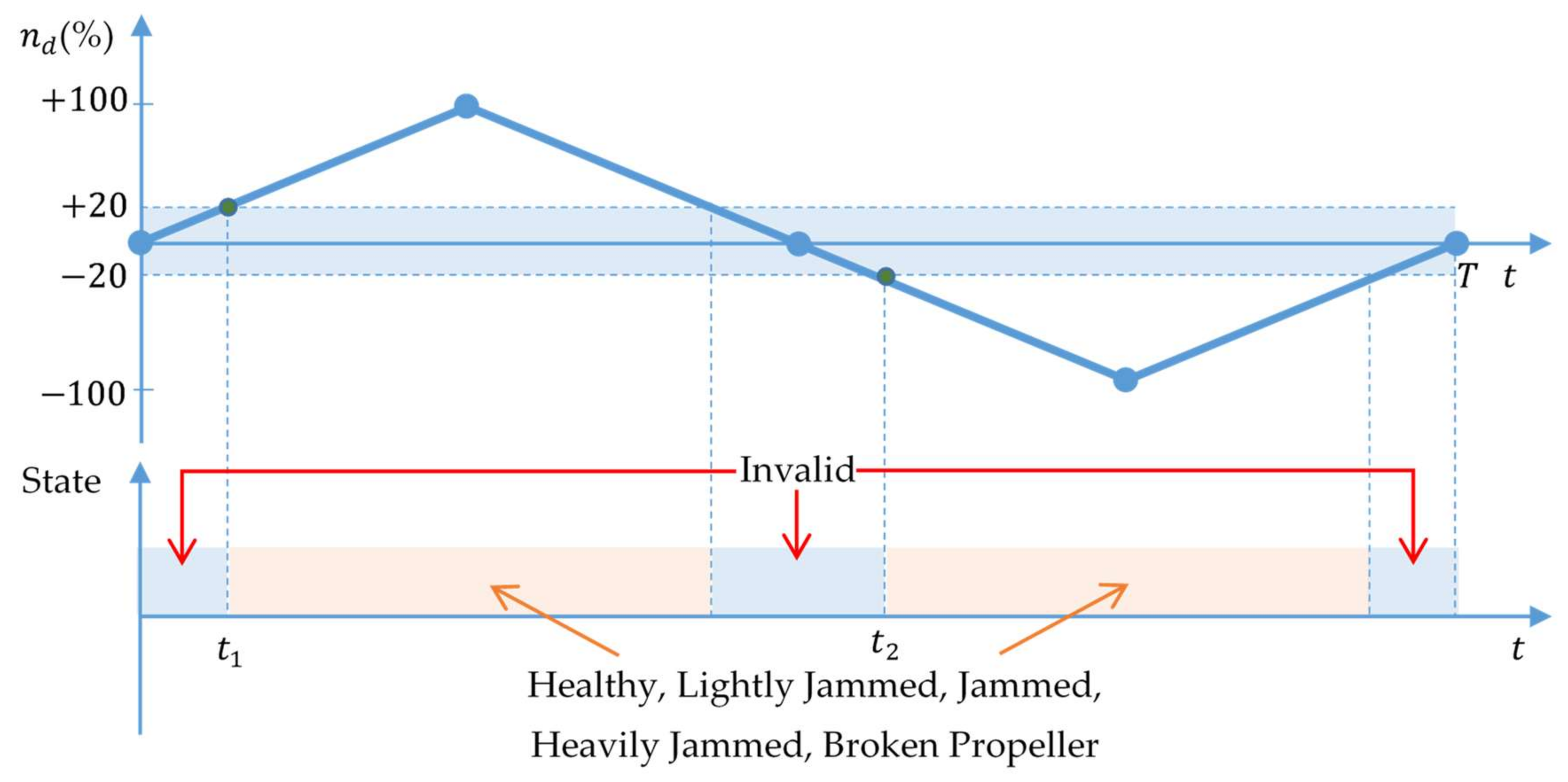
Analysing the distribution of the training data in Figure 5, the first feature that can be noticed is that each fault type creates a certain pattern. The presence of measurement noise is noticeable in acquired data for currents, resulting in patterns which exhibit a fuzzy (“cloudy”) look. The second feature is that it is very difficult to distinguish individual patterns in the zone around $n_d\approx 0$ (called the critical zone). This makes successful fault detection and isolation in the critical zone difficult to achieve. In particular, for the near-zero velocity case $n_d\approx 0$ the thruster does not rotate or rotates very slowly, reliable fault detection is impossible. The solution to this issue is the exclusion of the critical zone from FDI during the on-line fault detection phase. For this reason, the critical zone is called the forbidden zone with associated “Invalid” thruster state. When desired shaft speed is in this zone, the FDI algorithm goes to sleep mode and outputs the “Invalid” state without any action.

Each fault type in Figure 5 is characterised by specific features, which makes them different from the other types. These features are discussed in the following. In general, all the variables ($n_d$, $I$ and $n$) are correlated, i.e., they tend to rise and fall together in a non-linear way. For lightly jammed, jammed and heavily jammed propeller states, objects (“blockages”) attached to the blades generate an additional load for the motor, leading to higher current $I$ and lower $n$ than in the fault-free case for the same value of $n_d$. 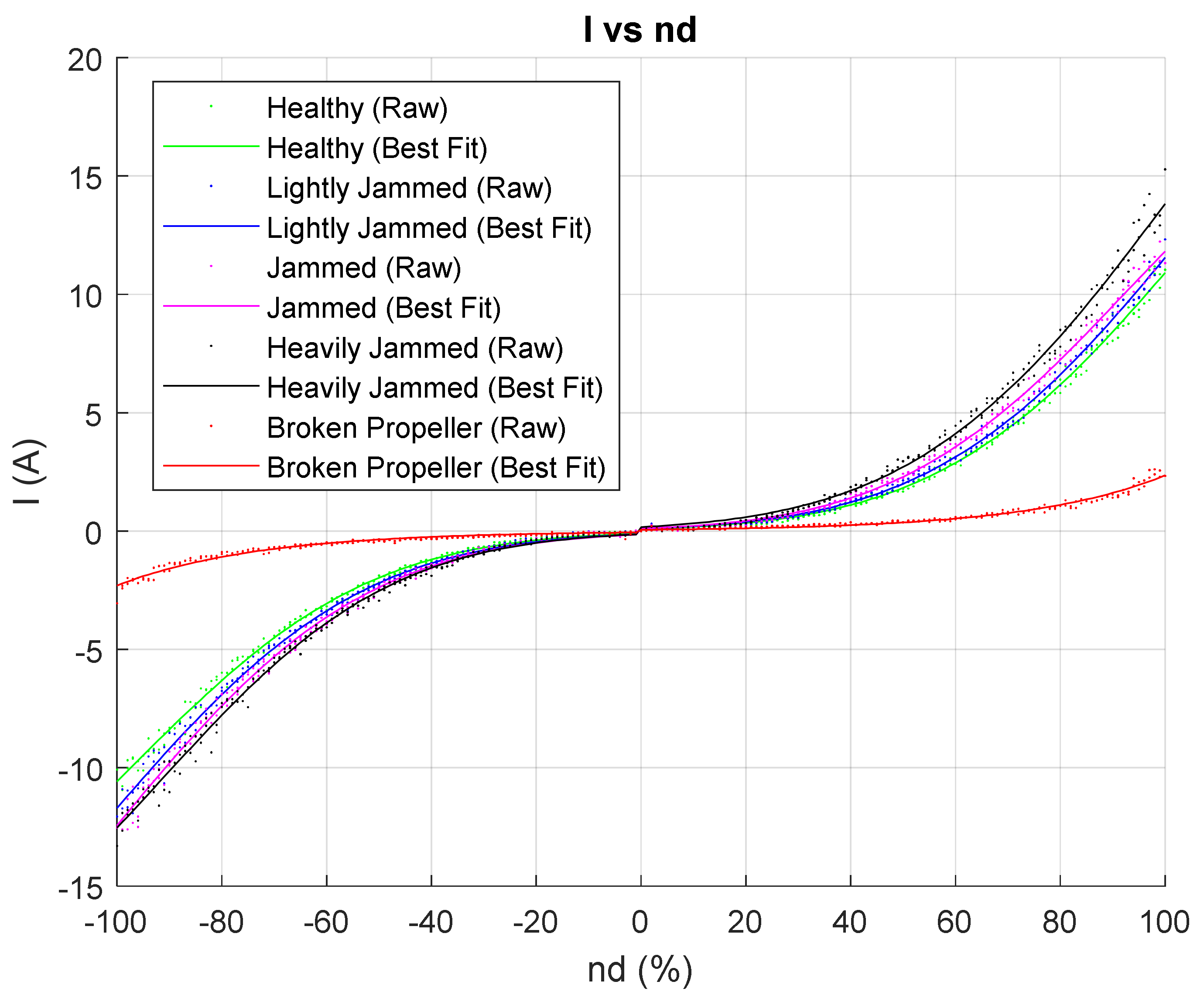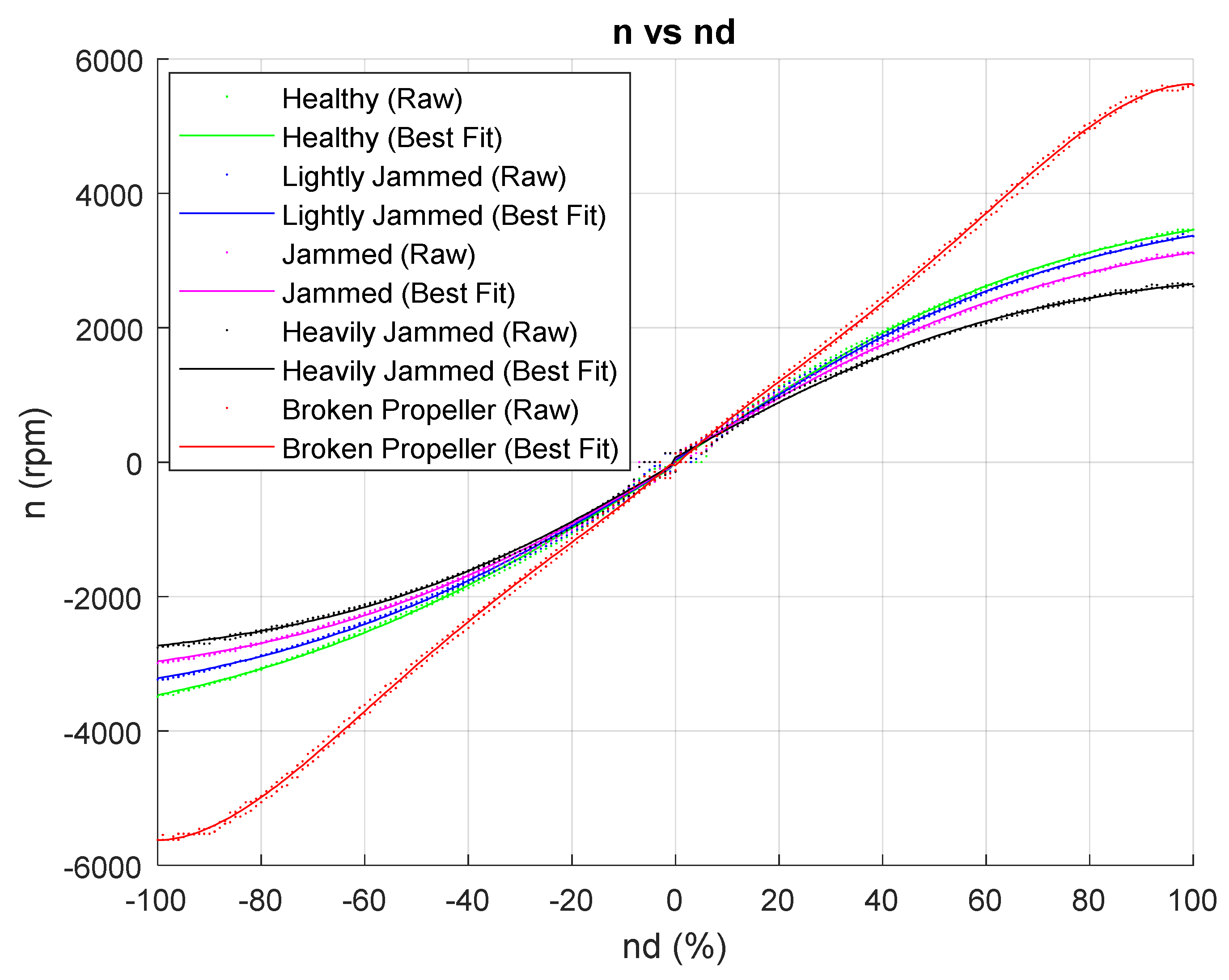In the case of a broken propeller, the absence of the blades means that the load for the motor is much smaller than in other cases, yielding a reduction in current consumption and a significant increase in shaft speed. However, the thruster does not generate any propulsion force in this case.

The main idea of the second stage in the training phase is to use the acquired data from the first stage to train a Pattern Recognition Neural Network (PRNN). In order to improve the PRNN classification accuracy, the raw data shown in Figure 5 have been first replaced with best fit curves, as shown in Figure 6 and Figure 7, before creating input-output data sets for NN training. The MATLAB App “Curve Fitting” has been employed to generate best fit curves. Details of the Curve Fitting functions and their parameters can be found in

Table 5. Curve Fitting functions for thruster states.

Thruster State Dataset Plot	Curve Fitting Function Type	Curve Fitting Function	Coefficients
Healthy I v $n_d$ positive	Gaussian	f(x) = a ∗ exp(−((x − b)/c)2)	a = 19.15
			b = 147.8
			c = 63.78
Healthy I v $n_d$ negative	Gaussian	f(x) = a ∗ exp(−((x − b)/c)2)	a = −16.07
			b = −140.2
			c = 62.24
Healthy n v $n_d$ positive	Hyperbolic tangent	f(x) = a ∗ tanh(b ∗ x) + c	a = 4008
			b = 0.01298
			c = 7.086
Healthy n v $n_d$ negative	Hyperbolic tangent	f(x) = a ∗ tanh(b ∗ x) + c	a = 4212
			b = 0.01134
			c = −42.63
Lightly Jammed I v $n_d$ positive	Gaussian	f(x) = a ∗ exp(−((x − b)/c)2)	a = 20.04
			b = 147.8
			c = 64.41
Lightly Jammed I v $n_d$ negative	Gaussian	f(x) = a ∗ exp(−((x − b)/c)2)	a = −19.26
			b = −145.9
			c = 65.05
Lightly Jammed n v $n_d$ positive	Hyperbolic tangent	f(x) = a ∗ tanh(b ∗ x) + c	a = 3908
			b = 0.01274
			c = 30.12
Lightly Jammed n v $n_d$ negative	Hyperbolic tangent	f(x) = a ∗ tanh(b ∗ x) + c	a = 3764
			b = 0.01237
			c = −37.82
Jammed I v $n_d$ positive	Gaussian	f(x) = a ∗ exp(−((x − b)/c)2)	a = 16.27
			b = 133.9
			c = 59.91
Jammed I v $n_d$ negative	Gaussian	f(x) = a ∗ exp(−((x − b)/c)2)	a = −20.4
			b = −146.1
			c = −65.54
Jammed n v $n_d$ positive	Hyperbolic tangent	f(x) = a ∗ tanh(b ∗ x) + c	a = 3565
			b = 0.01289
			c = 60.38
Jammed n v $n_d$ negative	Hyperbolic tangent	f(x) = a ∗ tanh(b ∗ x) + c	a = 3352
			b = 0.01355
			c = −29.18
Heavily Jammed I v $n_d$ positive	Gaussian	f(x) = a ∗ exp(−((x − b)/c)2)	a = 22.92
			b = 147.3
			c = 66.57
Heavily Jammed I v $n_d$ negative	Gaussian	f(x) = a ∗ exp(−((x − b)/c)2)	a = −17.17
			b = −134
			c = 60.65
Heavily Jammed n v positive	Hyperbolic tangent	f(x) = a ∗ tanh(b ∗ x) + c	a = 2875
			b = 0.01468
			c = 68.49
Heavily Jammed n v negative	Hyperbolic tangent	f(x) = a ∗ tanh(b ∗ x) + c	a = 3007
			b = 0.01488
			c = −14.55
Broken Propeller I v $n_d$ positive	Exponential	f(x) = a ∗ exp(b ∗ x)	a = 0.05542
			b = 0.03747
Broken Propeller I v $n_d$ negative	Exponential	f(x) = a ∗ exp(b ∗ x)	a = −0.05494
			$\mathrm{b}=-0.03735$
Broken Propeller n v $n_d$ positive	Polynomial	f(x) = p1 ∗ x4 + p2 ∗ x3 + p3 ∗ x2 + p4 ∗ x + p5	p1 = −0.0001074
			p2 = 0.01742
			p3 = −0.8264
			p4 = 72.56
			p5 = −46.07
Broken Propeller n v $n_d$ negative	Polynomial	f(x) = p1 ∗ x4 + p2 ∗ x3 + p3 ∗ x2 + p4 ∗ x + p5	p1 = 0.0001022
			p2 = 0.0163
			p3 = 0.7478
			p4 = 70.58
			p5 = 34.14

.

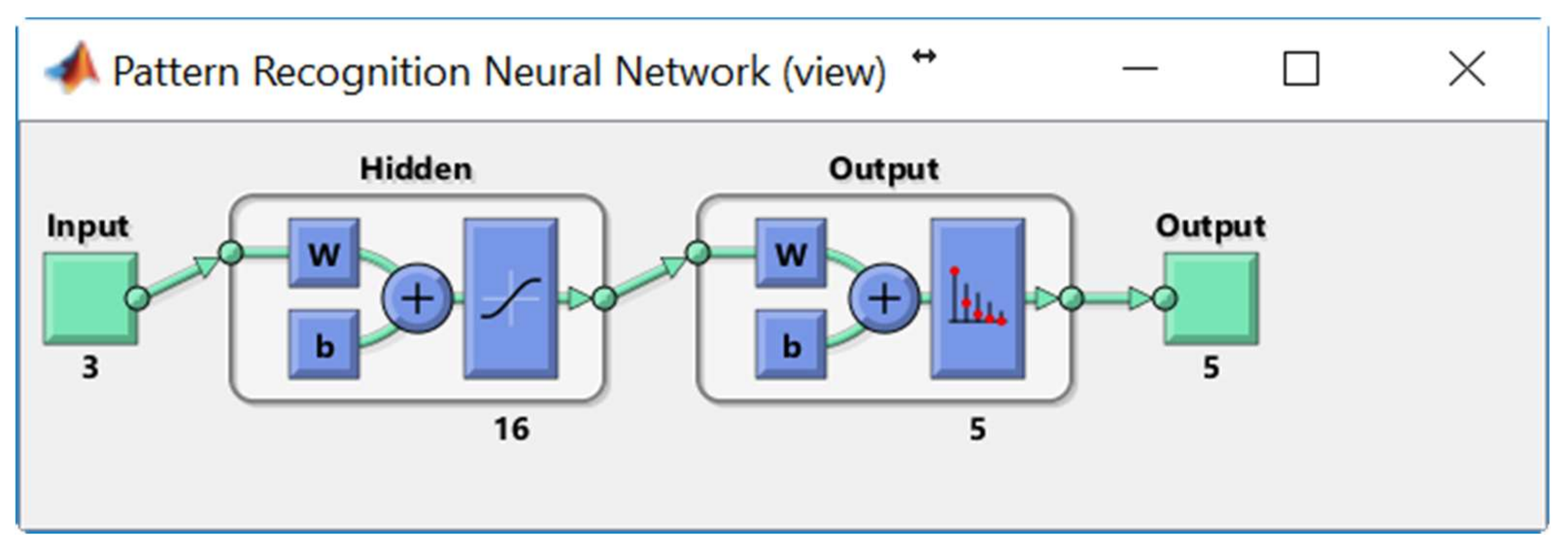
A two-layer feed-forward network, with 16 sigmoid hidden and 5 softmax output neurons has been trained to classify input vectors. The architecture of the Pattern Recognition Neural Network is shown in Figure 8.

As indicated in Table 4, there are five classes (Healthy, Lightly Jammed, Jammed, Heavily Jammed and Broken Propeller). The input data set (matrix thrusterInputs_RWE) has dimension 3 × 1005 and consists of five Input Blocks: thrusterInputs0_RWE, thrusterInputs1_RWE, thrusterInputs4_RWE (one block for each class, see

Table 6. Structure of the input training data set thrusterInputs_RWE.

Class	Input Block	Size	Column(j)
Healthy	thrusterInputs0_RWE	3 × 201	$n_d\left(j\right)$; $I\left(j\right)$; $n\left(j\right)$
Lightly Jammed	thrusterInputs1_RWE	3 × 201	$n_d\left(j\right)$; $I\left(j\right)$; $n\left(j\right)$
Jammed	thrusterInputs2_RWE	3 × 201	$n_d\left(j\right)$; $I\left(j\right)$; $n\left(j\right)$
Heavily Jammed	thrusterInputs3_RWE	3 × 201	$n_d\left(j\right)$; $I\left(j\right)$; $n\left(j\right)$
Broken Propeller	thrusterInputs4_RWE	3 × 201	$n_d\left(j\right)$; $I\left(j\right)$; $n\left(j\right)$

). Network inputs are stored in columns of the matrix thrusterInputs_RWE. For each class, values of $n_d$ are −100, −99, +99, +100.

The target data set (matrix thrusterTargets_RWE) has dimension 5 × 1005 and consists of five Target Blocks: thrusterTargets0_RWE, thrusterTargets1_RWE, thrusterTargets4_RWE (one block for each class, see

Table 7. Structure of the output training data set thrusterTargets_RWE.

Class	Target Block	Size	Column
Healthy	thrusterTargets0_RWE	5 × 201	1; 0; 0; 0; 0
Lightly Jammed	thrusterTargets1_RWE	5 × 201	0; 1; 0; 0; 0
Jammed	thrusterTargets2_RWE	5 × 201	0; 0; 1; 0; 0
Heavily Jammed	thrusterTargets3_RWE	5 × 201	0; 0; 0; 1; 0
Broken Propeller	thrusterTargets4_RWE	5 × 201	0; 0; 0; 0; 1

). For class k columns of corresponding Target Block have 1 at position k, while all other column elements have value 0.

Algorithms used in PRNN training are provided in

Table 8. Pattern Recognition Neural Network training algorithms.

Algorithms
Data Division	Random (dividerand)
Training	Scaled Conjugate Gradient (trainscg)
Performance	Cross-Entropy (crossentropy)
Calculations	MEX

.

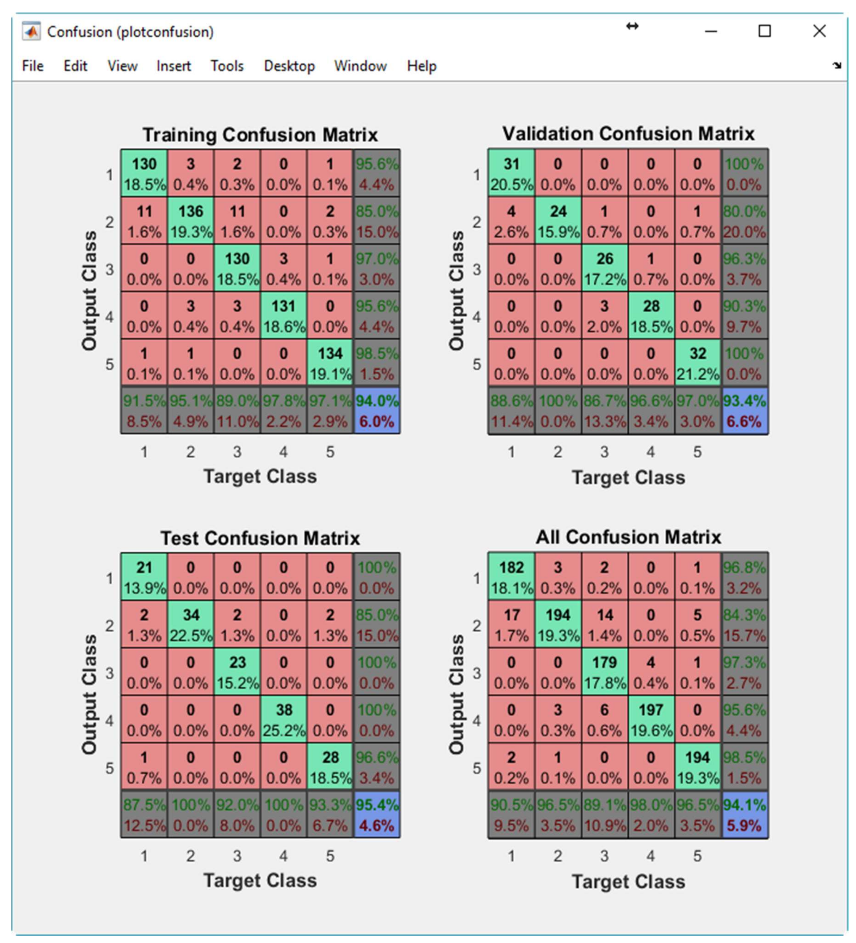
The input matrix thrusterInputs_RWE has been randomly divided up into training samples (70%), Validation samples (15%) and Testing samples (15%). These samples were presented to the network during training, and the network was adjusted according to its error. Validation samples were used to measure network generalization, and to halt training when the generalization stops improving. The testing samples have no effect on training and provide an independent measure of network performance during and after training. The training, Validation and Confusion Matrices are shown in Figure 9. On the confusion matrix plot, the rows correspond to the predicted class (Output Class), and the columns show the true class (Target Class). The diagonal cells show for how many (and what percentage) of the examples the trained network correctly estimates the classes of observations. That is, it shows what percentage of the true and predicted classes match. The off diagonal cells show where the classifier has made mistakes. The column on the far right of the plot presents the accuracy for each predicted class, while the row at the bottom of the plot shows the accuracy for each true class. The cell in the bottom right of the plot shows the overall accuracy.

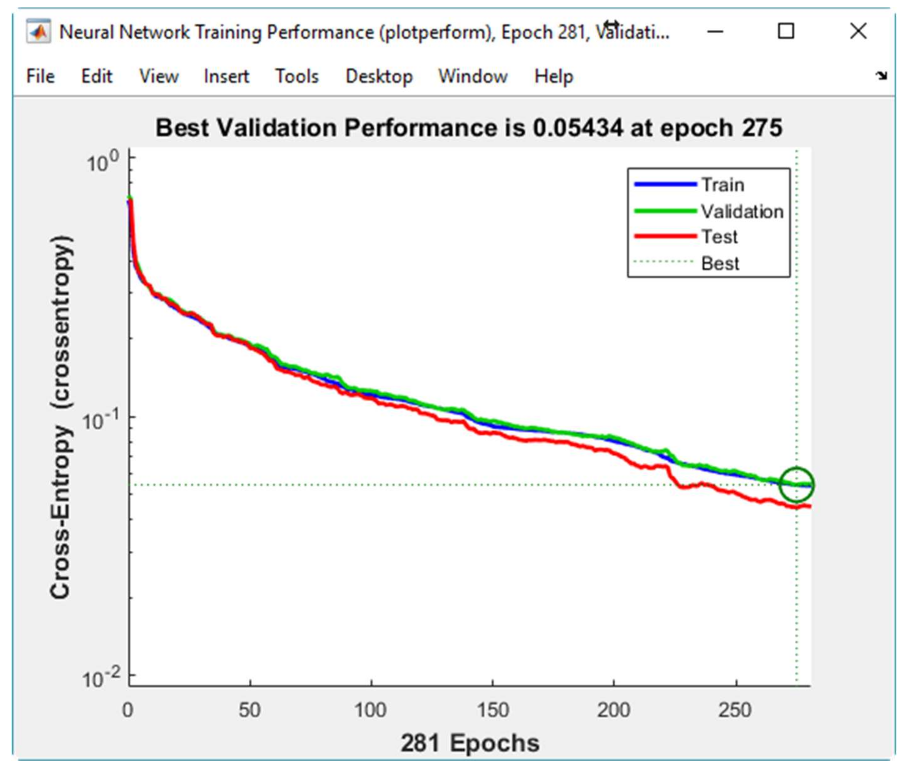
Figure 10 displays the Neural Network Cross-Entropy and Performance plots. Minimizing Cross-Entropy within the neural network results in enhanced classification.

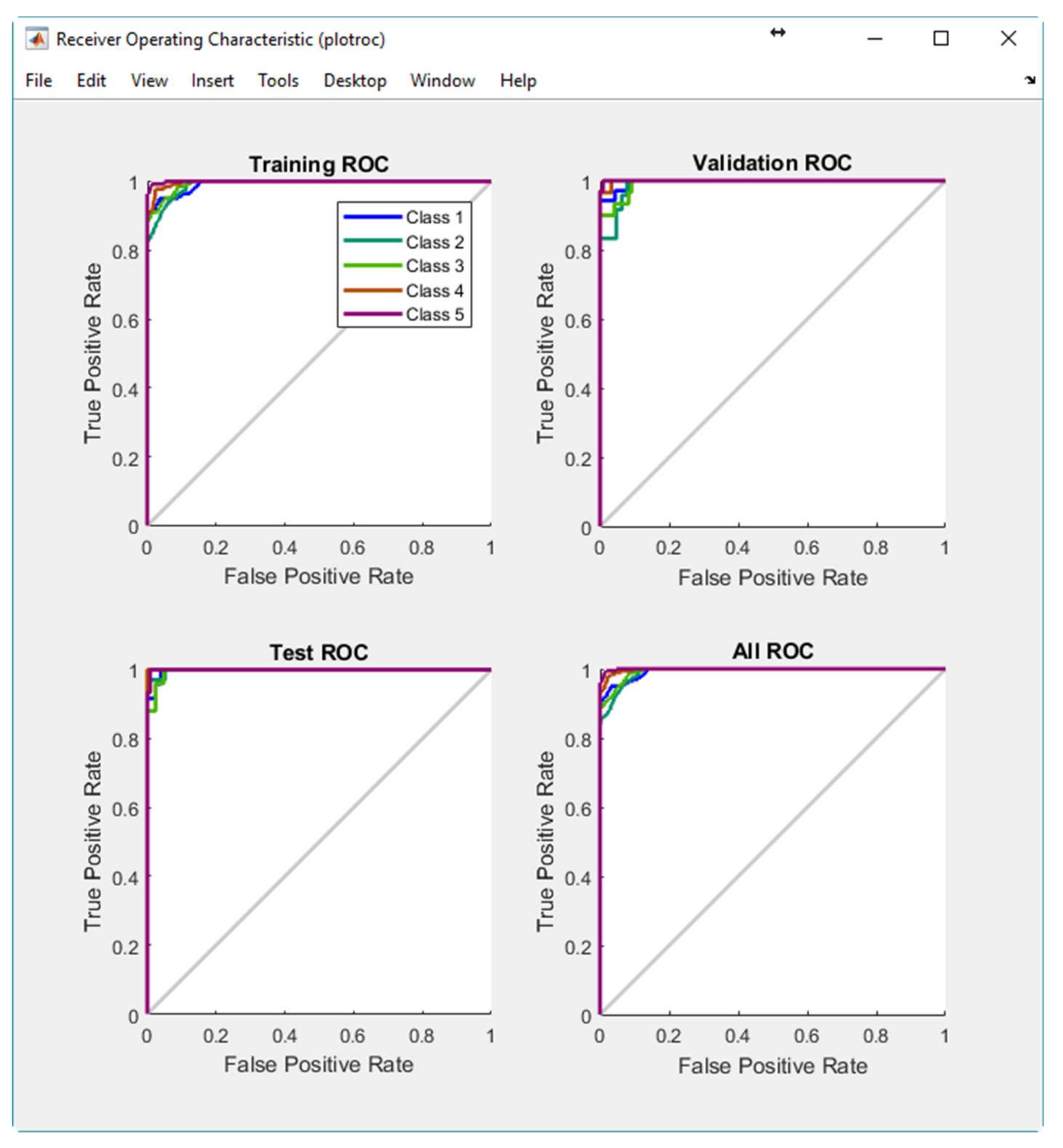
The Receiver Operating Characteristic (ROC) is a metric employed to check the quality of classifiers. For each class of a classifier, the ROC applies threshold values across the interval [0, 1] to outputs. For each threshold, two values are calculated, the True Positive Ratio (TPR) and the False Positive Ratio (FPR). For a particular class i, the TPR is the number of outputs whose actual and predicted class is class i, divided by the number of outputs whose predicted class is class i. The FPR is the number of outputs whose actual class is not class i, but predicted class is class i, divided by the number of outputs whose predicted class is not class i. Figure 11 displays the ROC for each output class of PRNN. The more each curve hugs the left and top edges of the plot, the better the classification.

The classification performance of the PRNN in the real-world environment is verified in Section 4.

In the third and last stage of the training phase, the structure of the trained PRNN is saved as a MATLAB function nn_pr_16_RWE on the hard disk for future use. In this way, time consuming training calculations are performed off-line, during the training phase, which enables fast and efficient detection during the on-line phase.

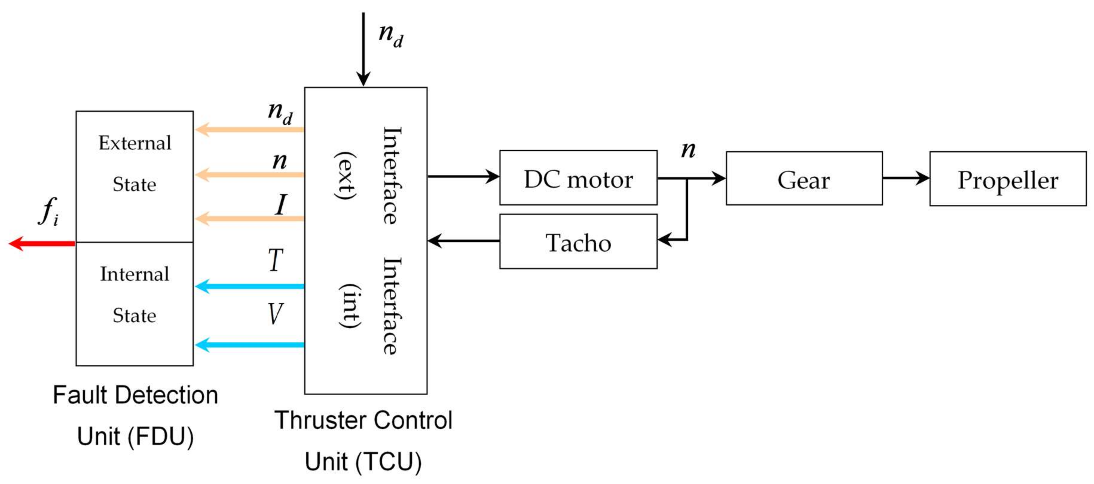
On-Line Fault Detection Phase

From the preceding discussion, the problem of thruster fault detection is considered as a pattern recognition problem. An original method for on-line fault detection, adapted to the specific features of the underlying pattern recognition problem, will now be described.

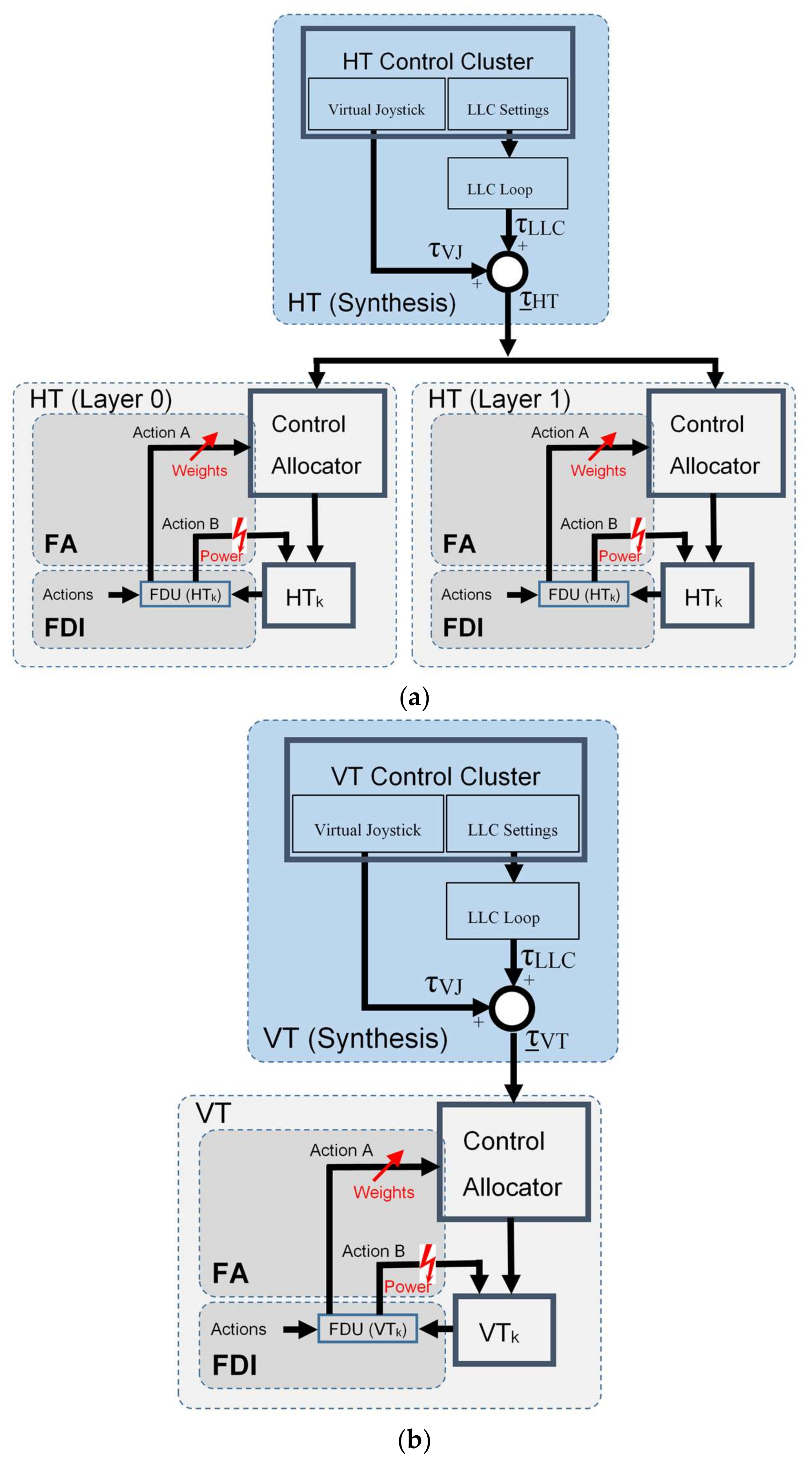
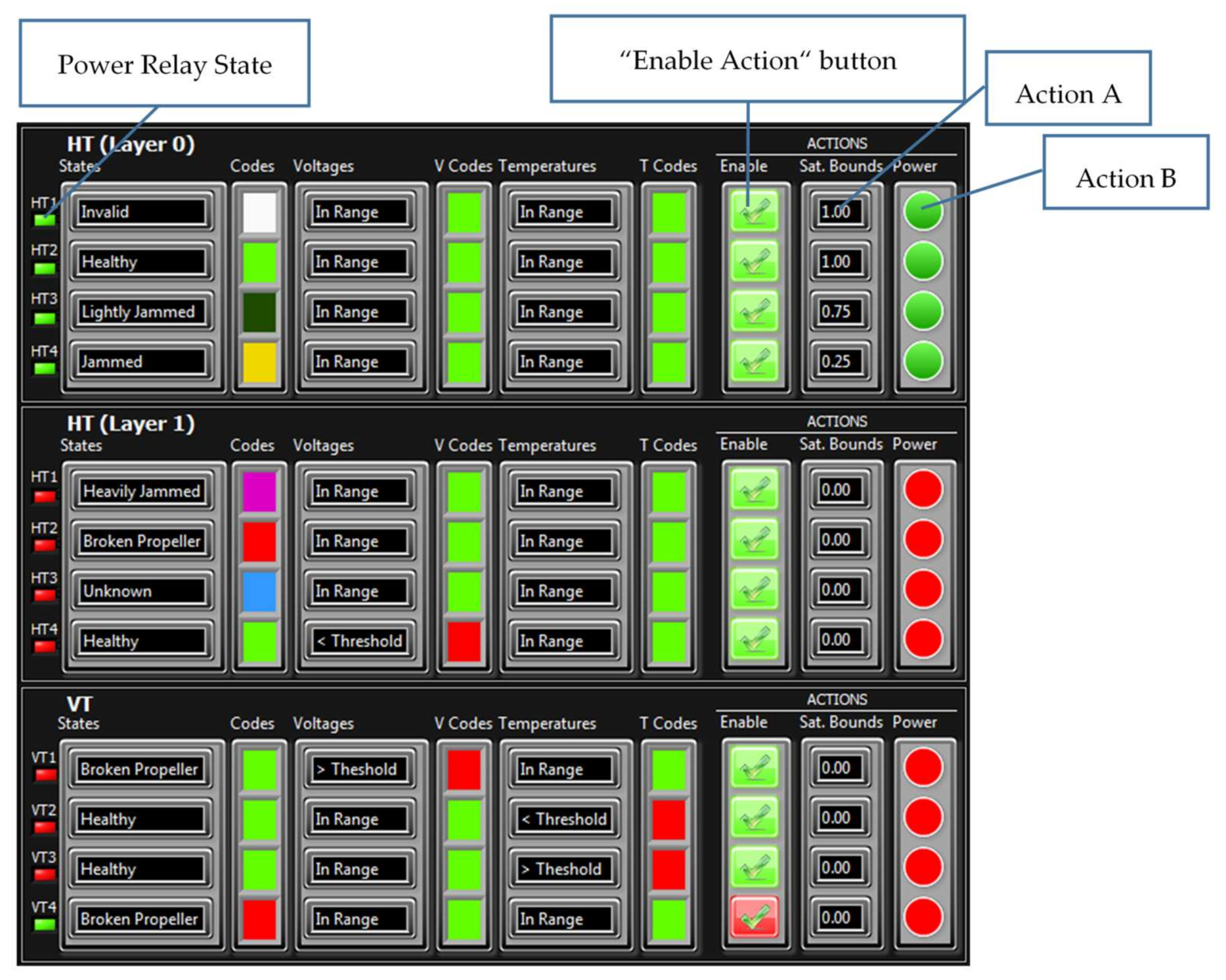
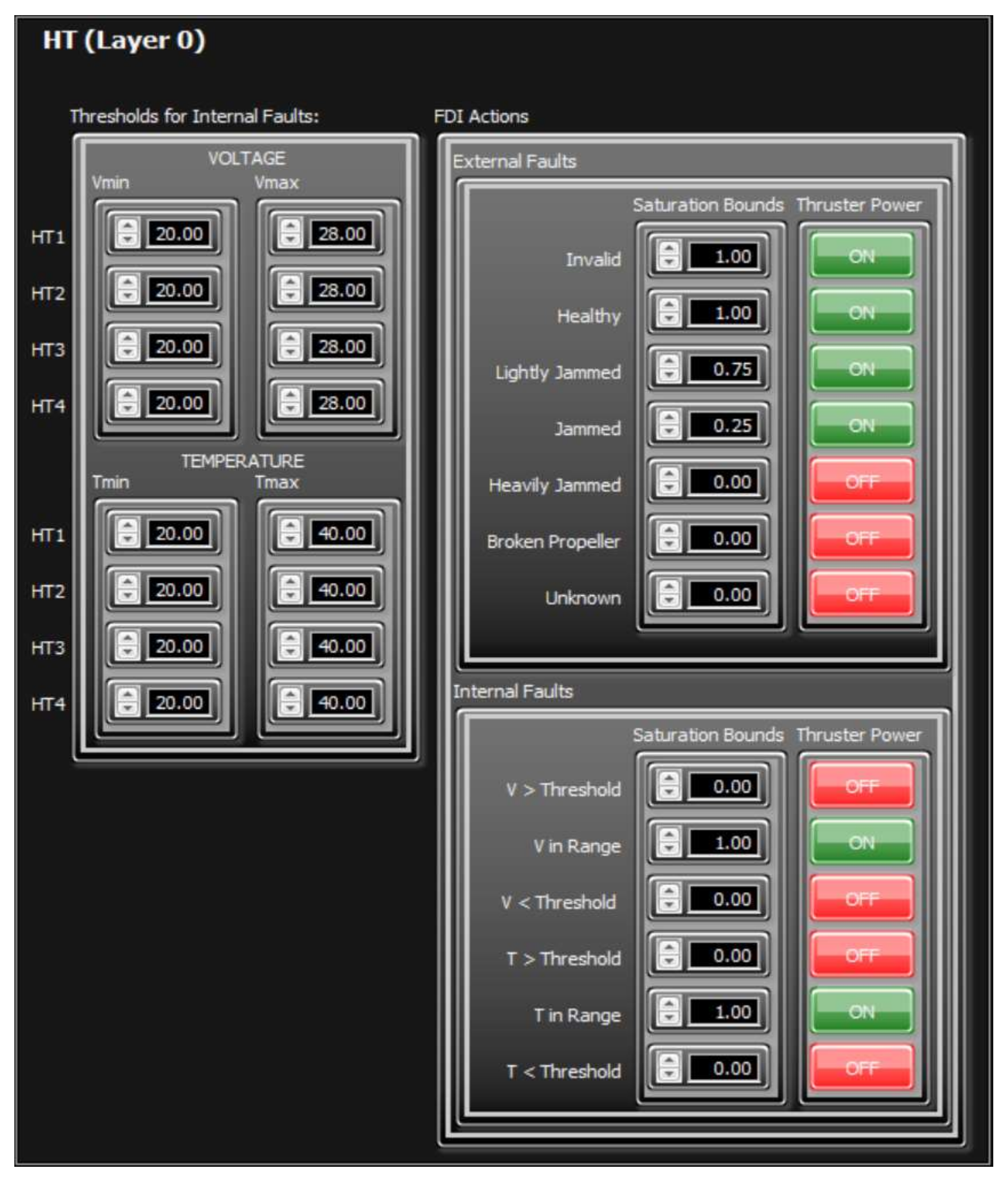
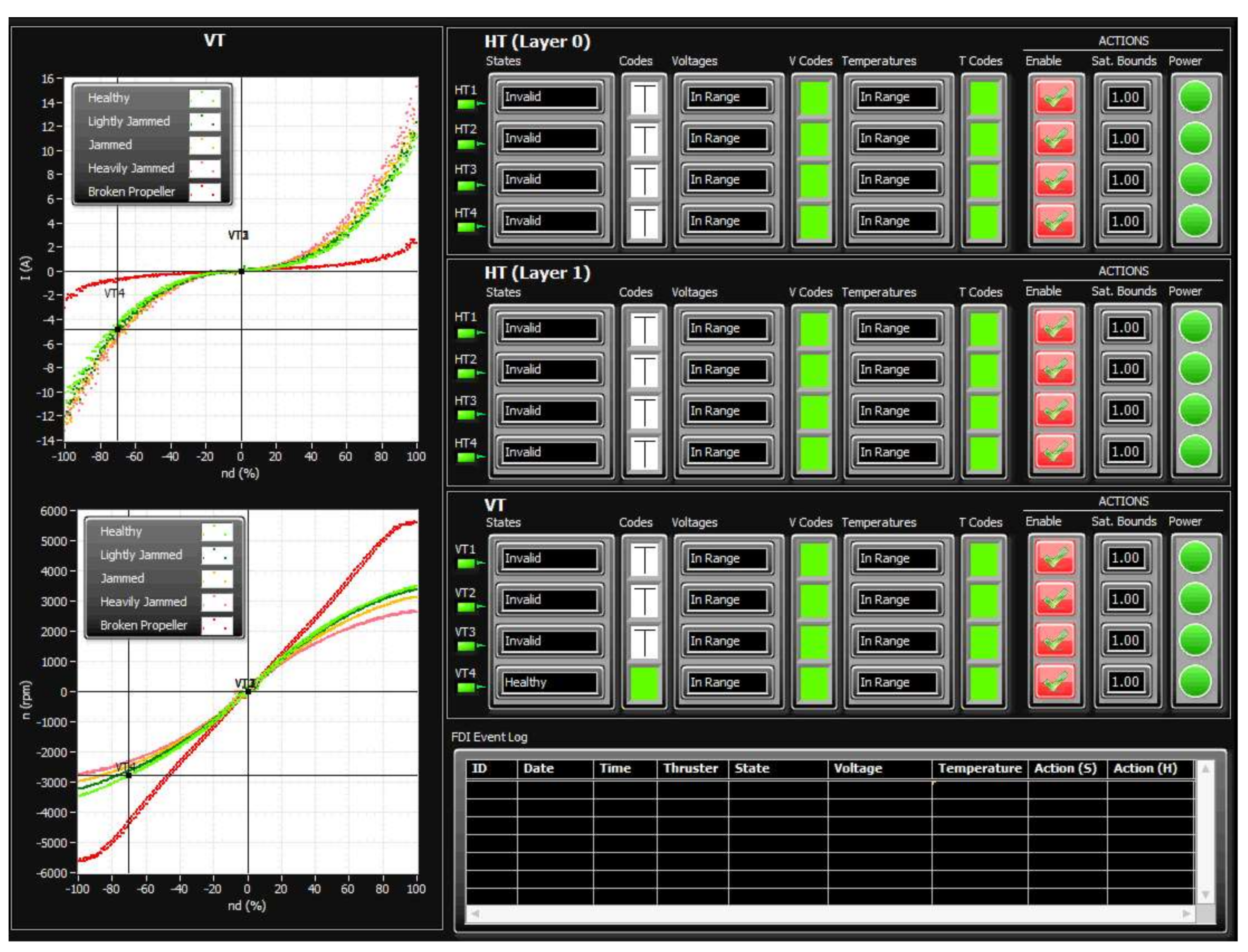
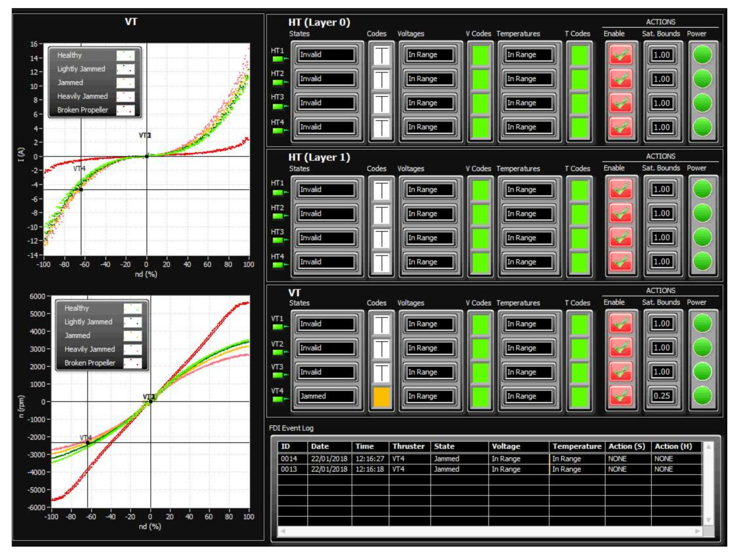
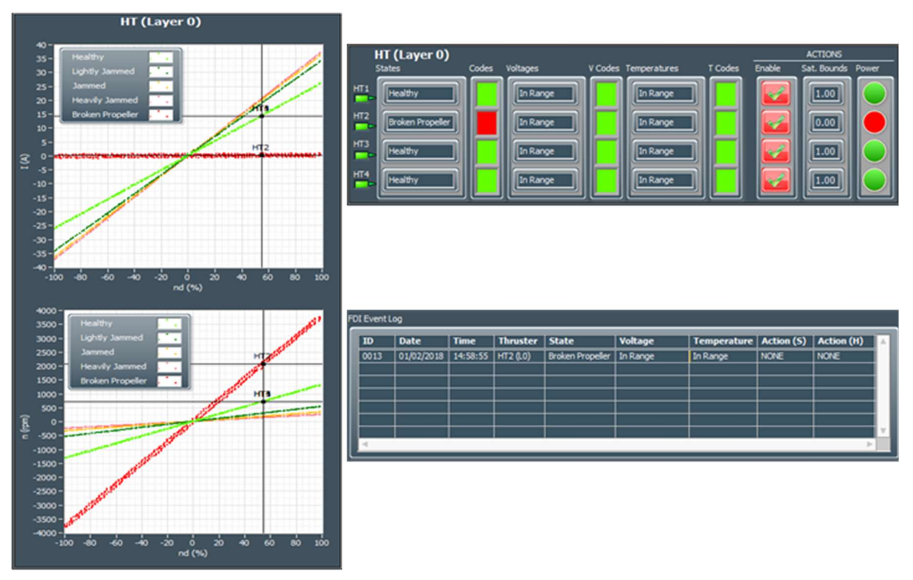
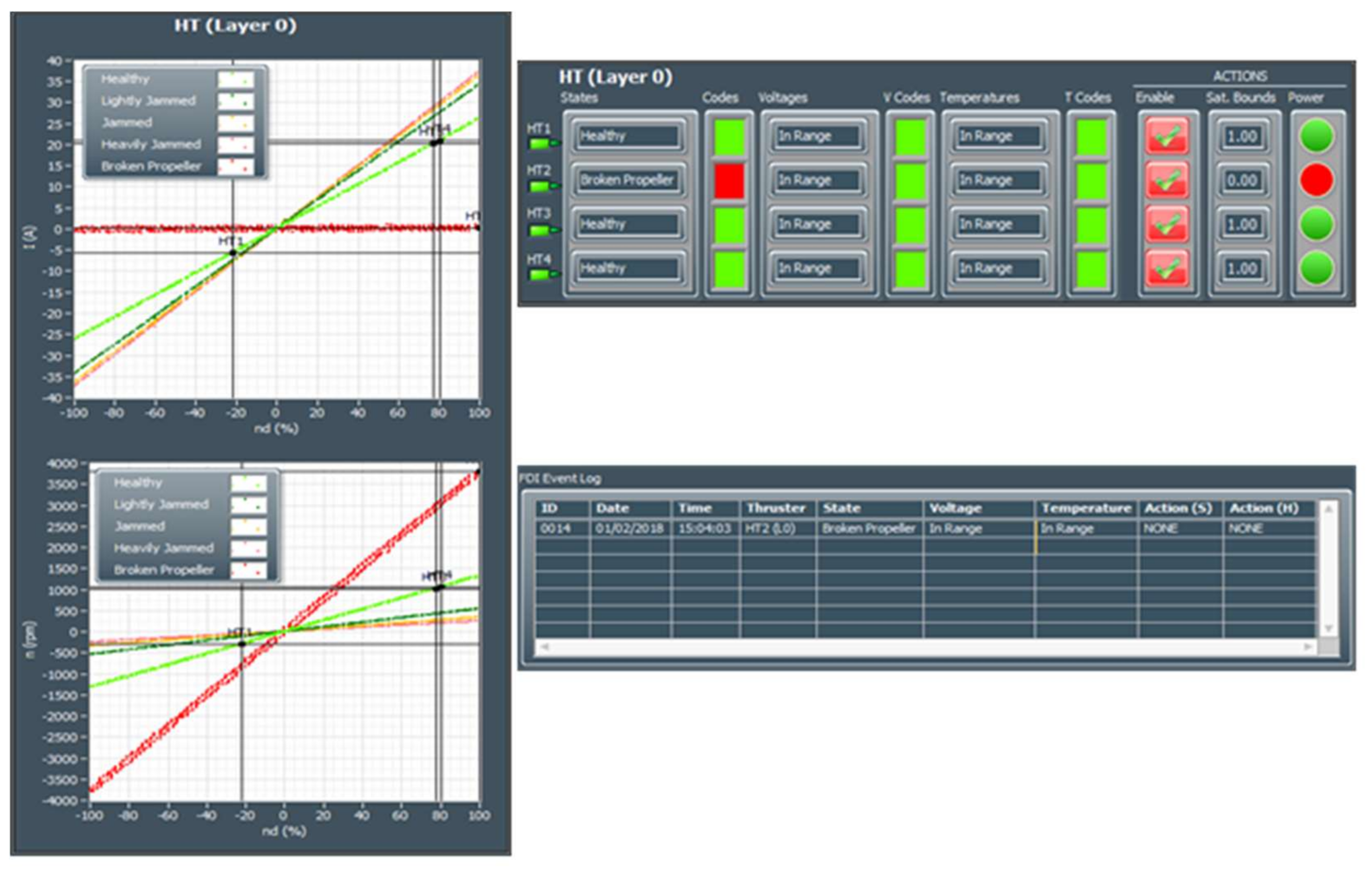
During the initialisation stage of the on-line fault detection phase, training data for each class (acquired in the off-line training phase) are loaded into memory and displayed as separate static background plots $I$ versus $n_d$ and $n$ versus $n_d$ for each layer (HT Layer 0, HT Layer 1 and VT Layer). These plots are utilised to represent the relationship between variables for different thruster states and for visualisation of actual thruster measurements in real-time. Additional activities during initialisation phase include memory allocation for buffers, reading fault code table settings from file and the creation of action lists.

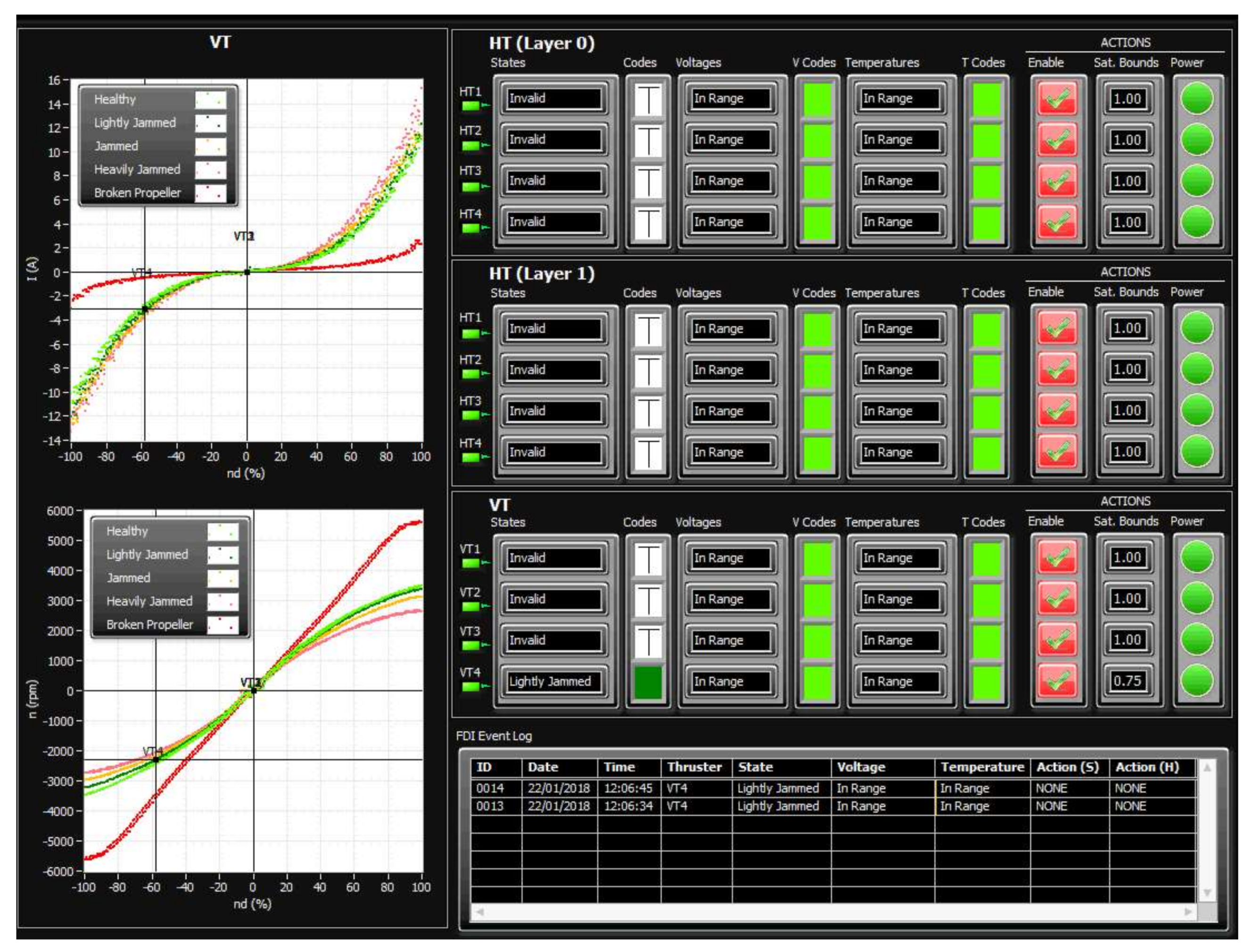
After the initialisation is finished, the fault detection is performed by repeating the steps from the FDU Algorithm (

Table 9. FDU Algorithm—On-line fault detection.

FDU Algorithm
1	Read values for external faults ($n_d$, $I$ and $n$) and internal faults ($V$ and $T$) from TCU.
2	Create vector $x={\left[\begin{array}{ccc}{n}_d& I& n\end{array}\right]}^T$ and execute $y=\mathrm{nn}\_\mathrm{pr}\_16\_\mathrm{RWE}\left(x\right); y=round\left(y\right);$ 1
3	Combine fault code table (Table 3) and thruster target table (Table 6) to determine thruster external fault state and corresponding actions A & B.
4	Determine internal fault state and actions A & B from thruster fault code table by examining if values of $V$ and $T$ exceed the limits.
5	(Optional) Use prioritisation scheme to resolve simultaneous appearance of external and internal faults: total faults have higher priority than partial faults.
6	Deliver the final thruster state and actions A & B as output.

¹ Vector y will have one of the following six values: [1; 0; 0; 0; 0], [0; 1; 0; 0; 0], [0; 0; 1; 0; 0], [0; 0; 0; 1; 0], [0; 0; 0; 0; 1], [0; 0; 0; 0; 0]. The last value is obtained in cases when a thruster operates in an unknown regime i.e., out-of-normal regime, different from faulty cases shown in Table 5. Typical examples for this case from the real-world environment include propeller jammed with rope or seaweed. The thruster state associated with value y = [0; 0; 0; 0; 0] is “Unknown” (see Thruster Fault Code Table in Table 3).

) for each thruster at each programme cycle.

It should be mentioned that, in order to avoid false detection due to outliers and measurement noise, the outputs of FDU Algorithm are buffered i.e., the final decision about thruster fault is not derived from a single measurement, but is accomplished using present and past thruster states (FDU Algorithm outputs), which are stored in the buffer. This buffer operates similar to the shift register: when the new state is pushed into the buffer, the other states are pushed (shifted) down and the ″oldest″ state is pushed (shifted) out. Elements of the buffer are compared to each other, and if all buffer elements have the same value (state), then the aggregate thruster state is set to this value. Otherwise, the previous value is kept as the aggregate state.

3.3. Fault Accommodation (FA) Subsystem

The proposed FA subsystem is an extension of the hybrid approach for control allocation based on integration of the pseudoinverse and the fixed-point iteration method which compensates the thruster fault effect [15,16]. It is implemented as a two-step process. The pseudoinverse solution is found in the first step. Then the feasibility of the solution is examined, analysing its individual components. If violation of actuator constraint(s) is detected, the fixed-point iteration method is activated in the second step. In this way, the hybrid approach is able to allocate the exact solution, optimal in the l₂ sense, inside the entire attainable command set. This solution minimises a control energy cost function, the most suitable criteria for underwater applications.

As stated in Section 3.1, the HT Synthesis and VT Synthesis modules create virtual control vectors ${\tau }_{HT}$ and ${\tau }_{VT}$. These vectors represent the total control effort (normalised forces and moments) to be produced by the actuators (thrusters). Control Allocators in Figure 2 find individual actuator settings (true control vectors $u_{HT}$ and $u_{VT}$ for horizontal and vertical thrusters, respectively) to be applied in order to produce desired control effort. The Fault Accommodation (FA) subsystem uses FDI outputs (aggregate thruster states) and associated software-level actions (action A) and hardware-level actions (action B) to solve the control allocation problem for each thruster layer in presence of partial/total thruster faults. Action A (see Table 3) includes penalisation of faulty thruster in the solution of control allocation problem by restricting saturation bounds i.e., by increasing the corresponding weight in the weighting matrix [16]. Action B includes power isolation of faulty thrusters (total faults only in Table 3) such that the entire ROV power system is not compromised. Hence, if the aggregated thruster state is a partial fault, the thruster is penalised, but will continue to operate. However, in the case of a total fault, the thruster is removed from the control allocation process, and its power is switched off in parallel.

3.4. Software Implementation

The proposed FTC has been implemented as a LabVIEW VI named “Thruster Active FDI”, which is a software module integrated with other OceanRINGS⁺ modules. The user interface, which shows FDI results, is presented in Figure 12. This image is just an example; it has been artificially generated by injecting faults in the simulated thruster models, and it is intended to illustrate various options available in the software to detect, isolate and accommodate faults. The display is divided into 3 groups: horizontal thrusters (Layer 0 & Layer 1) and vertical thrusters. Each state has an associated colour code box. The external faults are represented with a column named “States”, while internal faults are displayed as columns named “Voltages” and “Temperatures”. The fault code table for the individual layers can be edited on the configuration tab of the main application. The fault code table for the horizontal thrusters (Layer 0) can be viewed in Figure 13.

In order to increase the flexibility of the proposed FTC scheme, each thruster has associated individual “Enable Action” buttons. If the “Enable Action” is true, actions A & B will be applied. If the “Enable Action” is false, no actions will be applied i.e., the FDI subsystem will detect fault, but no action will be executed by the FA subsystem.

Thrusters HT1, HT2, HT3 & HT4 in Layer 0 in Figure 12 have “Enable Action” buttons set to true. The FDI subsystem has detected external faults (partial faults) in HT3 (Lightly Jammed) and HT4 (Jammed) and no presence of internal faults. All four thrusters remain powered on, while the software-level actions resulted in Saturation Bounds set to 0.75 and 0.25 for HT3 and HT4, respectively.

In a similar way, thrusters HT1, HT2, HT3 & HT4 in Layer 1 in Figure 12 have “Enable Action” buttons set to true. In this case, the FDI has detected external faults (total faults) in HT1 (Heavily Jammed), HT2 (Broken) and HT3 (Unknown), and presence of an internal fault in HT4 (Voltage < Threshold). Hardware-level actions resulted that the power to all four thrusters is switched off (as was confirmed by the power relay states for HT1–HT4, Layer 1), while software-level actions resulted in Saturation Bounds set to 0 for all four thrusters.

Finally, thrusters VT1, VT2 & VT3 have “Enable Action” buttons set to true. The FDI has detected external fault (total fault) in VT1 (Broken Propeller), and internal faults (total faults) in VT2 (Temperature < Threshold) and VT3 (Temperature > Threshold). Hardware-level actions resulted that the power to all three thrusters is switched off (as confirmed by Power Relay States), while software-level actions resulted in Saturation Bounds set to 0 for all three thrusters. Thruster VT4 has “Enable Action” button set to false. The FDI has detected an external fault (total fault) in VT4 (Broken Propeller) and no presence of internal faults. However, the FA subsystem did not execute action A (set Saturation Bounds to 0) and action B (switch off power to the thruster, as confirmed with power relay state for VT4).

An event log table is used to log Fault Detection and Isolation (FDI) events i.e., details of thruster external and internal faults as they occur. The FDI Event Log Table data includes event I.D., date and timestamp of fault occurrence, thruster in which fault occurred, type of external and internal fault and, if the “Enable Action” button is set to true, the software-level and hardware-level actions that were applied. An example of the FDI Event Log Table is shown in Figure 14.

4. Testing and Evaluation of the FTC

The performance of the FTC, proposed and described in Section 3, is evaluated and tested in a real-world and virtual (simulated) environment. In the real-world environment, a single M5 VideoRay thruster has been utilised to evaluate the FTC performance for various fault conditions. In the virtual (simulated) environment, various thruster fault conditions were simulated in order to examine the behaviour of the FTC in different situations (open-loop/closed-loop control performance with enabled/disabled FA actions).

4.1. Evaluation of the FTC in Real-World Environment

A single M5 VideoRay thruster, configured as VT4, has been used for post-training validation of the trained PRNN and to evaluate the performance of the FTC in fault-free mode (no object attached to the propeller) and faulty modes (with “blockages” of various sizes and shapes attached to the blades, see Figure 4). The main objective was to evaluate the capability of the FDI subsystem to detect thruster states for external faults only, with a disabled FA subsystem (the “Enable Action” button set to false for VT4). The thruster was actuated with the same signal that has been used to acquire training data (Figure 15) i.e., with saw-like command signal $n_d$ (%) with the following pattern: 0% » MAX% » 0% » −MAX% » 0%, step size 1%. The total duration of signal was T = 20 s, sampling period 50 ms and max. value MAX = 100%. The critical (forbidden) zone has been set to $n_d\in \left[-20\%, 20\%\right]$. Screenshots of the FDI results for various thruster states are shown in Figure 16, Figure 17, Figure 18, Figure 19 and Figure 20. Note that the results are for VT4 only. All other thruster states are shown as Invalid.

The FDI subsystem registers events only when the command signal $n_d$ leaves the critical (forbidden) zone. Two events have been logged for each fault: the Event 1 with timestamp $t_1$ (time instance when the command signal $n_d$ left the critical zone for the first time, see Figure 15), and the Event 2 with timestamp $t_2$ (time instance when the command signal $n_d$ left the forbidden zone for the second time). While passing through the forbidden zone, the FDI subsystem went to “sleep” mode indicating a thruster state = “Invalid”. The PRNN correctly recognised a thruster state outside the forbidden zone in all five cases. Test results confirmed that the PRNN has 100% classification accuracy outside the forbidden zone, and that the miss-classification appears exclusively inside the critical (forbidden) zone, as predicted in Section 3.1.

4.2. Evaluation of the FTC in Virtual (Simulated) Environment

As mentioned in Section 3.2, in the virtual (simulated) environment thruster faults are simulated by varying properties of the thruster dynamic model (load, friction, etc.) inside the propulsion subsystem of the ROV dynamics simulator. Off-line training and on-line fault detection phases are performed in the same way as described in Section 3.2 for the real-time environment but, in this case, faults are simulated by varying efficiency of thruster or by pushing the “Broken Propeller” button on the Thruster Configuration tab, shown in Figure 21.

A description of the simulation test cases, presented in this section, is given in

Table 10. Description of simulation tests.

ID	Type	LLC Settings	Thruster	Fault	“Enable Action”
1	Open-Loop		HT2 (L0)	Broken Propeller	False
	${\tau }_X\left(VJ\right)=0.3$	Heading: OFF
	${\tau }_Y\left(VJ\right)=0.0$	Surge Speed: OFF
	${\tau }_N\left(VJ\right)=0.0$	Sway Speed: OFF
2	Closed-Loop	vd = proj(SOGd)y	HT2 (L0)	Broken Propeller	False
	$SO{G}_d=0.54 \mathrm{m}/\mathrm{s}$	ud = proj(SOGd)x
	$CO{G}_d={60}^{°}$	Yd = COGd
3	Closed-Loop	Yd = COGd	HT2 (L0)	Broken Propeller	True
	$SO{G}_d=0.54 \mathrm{m}/\mathrm{s}$	ud = proj(SOGd)x
	$CO{G}_d={60}^{°}$	vd = proj(SOGd)y

.

The test cases described in Table 10 enable investigation of the influence of thruster faults on the overall control performance of the ROV and demonstrate the ability of the FTC to accommodate the faults and minimise the negative impact on control performance. It should be emphasized that similar test cases have been conducted with total and partial faults in vertical thrusters, and the main conclusion is that the ROV control system with active FDI and FA subsystems is capable of maintaining full 3 DOF in the vertical plane in the presence of a partial or total fault in a single vertical thruster.

4.2.1. Test 1: Impact of “Broken Propeller” in Open-Loop Mode with Disabled Fault Accommodation

In this case, the Surge, the Sway and the Yaw LLCs are disabled and the virtual control vector ${\tau }_{HT}={\left[\begin{array}{ccc}0.3& 0.0& 0.0\end{array}\right]}^T$ is constant during the duration of the test. At time instance $t_0$ the “Broken Propeller” fault occurs in HT2, Layer 0. The FDI subsystem detects the fault and logs the FDI event, but the FA subsystem does not perform any action, since the “Enable Action” button is set to false (Figure 22). For this reason, the Control Allocator still assumes that the thruster HT2 is healthy and does not modify the solution of the control allocation problem. However, since HT2 does not produce any thrust/moment, the ROV drifts to the right side, with continuous change in heading (Figure 23).

4.2.2. Test 2: Impact of “Broken Propeller” in Closed-Loop Mode with Disabled Fault Accommodation

In this case, the Surge, the Sway and the Yaw LLCs are enabled, while all components of the Virtual Joystick vector are set to zero. The Speed Mode is set to SM2 (Follow Speed and Course) and the Heading Mode is set to HM2 (Follow Course). The Desired Speed Over Ground (SOG_d) is set to 0.54 m/s, and Desired Course Over Ground (COG_d) is set to 60°. The set points u_d for Surge Speed LLC and v_d for Sway Speed LLC are found as projections of the velocity vector in the horizontal plane on the x and y axis of the body-fixed {b} frame. At time instance $t_0$ the “Broken Propeller” fault occurs in HT2, Layer 0. The FDI subsystem detects the fault and logs the FDI event, but the FA subsystem does not perform any action, since the “Enable Action” button is set to false (Figure 24). Similar to Test 1, the Control Allocator still assumes that the thruster HT2 is healthy. However, robustness of closed-loop low-level controllers limit the ROV drift to the starboard side with a heading offset of 4.833° (Figure 25).

4.2.3. Test 3: Impact of “Broken Propeller” in Closed-Loop Mode with Enabled Fault Accommodation

Similar to Test 2, the Surge, the Sway and the Yaw LLCs are enabled, all components of Virtual Joystick vector are set to zero, the Speed Mode is set to SM2 (Follow Speed and Course) and the Heading Mode is set to HM2 (Follow Course). At time instance $t_0$ the “Broken Propeller” fault occurs in HT2, Layer 0. Since the “Enable Action” button is set to true (Figure 26), the FDI subsystem detects the fault and logs the FDI event, and the FA subsystem sets Saturation Bounds to zero for HT2 (action A) and switches off the thruster power (action B). The Control Allocator penalises (excludes) the faulty thruster in the solution of the control allocation problem and reallocates control energy among the operable thrusters (Figure 27). Small changes in the surge & sway speeds and heading are visible during the transient stage. The appearance of these transients is unavoidable, since operable thrusters need time to spin to new setpoints. However, after a short time period, all these changes diminish and the ROV continues in a straight-line motion, following the desired speed and course without error (Figure 27).

5. Conclusions and Future Work

This paper described a novel thruster fault-tolerant control system (FTC) for open-frame remotely operated vehicles (ROVs), developed by researchers at the Centre for Robotics & Intelligent Systems (CRIS), University of Limerick. The proposed FTC system is part of the OceanRINGS+ ROV smart control system, currently under development.

The proposed FTC consists of two subsystems: a model-free thruster fault detection and isolation subsystem (FDI) and a fault accommodation subsystem (FA). The FDI subsystem employs fault detection units (FDUs), associated with each thruster, to monitor their state. The robust, reliable and adaptive FDUs use a model-free pattern recognition neural network (PRNN) to detect internal and external faulty states of thrusters in real time. The FA subsystem combines information provided by the FDI subsystem with predefined, user-configurable actions to accommodate partial and total faults and to perform an appropriate control reallocation. Software-level actions include penalisation of faulty thrusters in solution of the control allocation problem and reallocation of control energy among the operable thrusters. Hardware-level actions include power isolation of faulty thrusters (total faults only) such that the entire ROV power system is not compromised.

Using simulations and real-world tests, the performance of the FTC was evaluated through a series of representative test cases, in order to examine the behaviour of the FTC in fault-free and faulty conditions. In the real-world environment, a single M5 VideoRay thruster has been used to evaluate the FTC performance for various fault conditions. Test results confirmed that the PRNN has 100% classification accuracy outside the forbidden zone, and that the miss-classification appears exclusively inside the critical (forbidden) zone. In the virtual (simulated) environment, various thruster fault conditions were simulated in order to examine the behaviour of the FTC in different situations (open-loop/closed-loop control performance with enabled/disabled FA actions). Simulation results show that the FTC provides automatic reallocation in faulty conditions, keeping all the DOF in the horizontal plane fully controllable and providing the opportunity to continue the mission with a minimal loss of control performance.

In the worst case scenario, the proposed FTC is able to maintain full 6 DOF control of the ROV in presence of up to 6 simultaneous total faults in thrusters (one layer with four horizontal thrusters fully disabled plus one disabled thruster in the other layer of horizontal thrusters plus one disabled vertical thruster).

Future work includes extension of the proposed FTC to interface with other ROVs and development of a “passive” method for fault detection and isolation for ROVs with thrusters that cannot provide active real-time monitoring of relevant signals from thrusters (currents, shaft speeds, applied voltages and temperatures of windings).

References

1. Capocci, R.; Dooly, G.; Omerdić, E.; Coleman, J.; Newe, T.; Toal, D. Inspection-class remotely operated vehicles—A review. J. Mar. Sci. Eng. 2017, 5, 13. [Google Scholar] [CrossRef]
2. O’Connor, M.; Lewis, T.; Dalton, G. Weather window analysis of Irish west coast wave data with relevance to operations & maintenance of marine renewables. Renew. Energy 2013, 52, 57–66. [Google Scholar]
3. Podder, T.K.; Antonelli, G.; Sarkar, N. Fault tolerant control of an autonomous underwater vehicle under thruster redundancy: Simulations and experiments. In Proceedings of the 2000 ICRA, IEEE International Conference on Robotics and Automation, Millennium Conference, Symposia Proceedings (Cat. No. 00CH37065), San Francisco, CA, USA, 24–28 April 2000; Volume 2, pp. 1251–1256. [Google Scholar]
4. Caccia, M.; Bono, R.; Bruzzone, G.; Bruzzone, G.; Spirandelli, E.; Veruggio, G. Experiences on Actuator Fault Detection, Diagnosis and Accommodation for ROVs. In International Symposium Unmanned Untethered Submersible Technology; University of New Hampshire, Marine Systems Engineering Laboratory: Durham, NH, USA, 2001. [Google Scholar]
5. Kim, J.H.; Beale, G.O. Fault Detection and Classification in Underwater Vehicles Using the T2 Statistic. Autom. J. Control Meas. Electron. Comput. Commun. 2002, 43, 29–37. [Google Scholar]
6. Montazeri, M.; Kamali, R.; Askari, J. Fault diagnosis of autonomous underwater vehicle using neural network. In Proceedings of the 2014 22nd Iranian Conference on Electrical Engineering (ICEE), Tehran, Iran, 20–22 May 2014; pp. 1273–1277. [Google Scholar]
7. Zhu, D.; Liu, Q.; Yang, Y. An Active Fault-Tolerant Control Method of Unmanned Underwater Vehicles with Continuous and Uncertain Faults. Int. J. Adv. Robot. Syst. 2008, 5, 1729–8806. [Google Scholar] [CrossRef]
8. Huang, H.; Wan, L.; Chang, W.-T.; Pang, Y.-J.; Jiang, S.-Q. A Fault-tolerable Control Scheme for an Open-frame Underwater Vehicle Regular Paper. Int. J. Adv. Robot. Syst. 2014, 11, 77. [Google Scholar]
9. Omerdić, E.; Roberts, G. Thruster fault diagnosis and accommodation for open-frame underwater vehicles. Control Eng. Pract. 2004, 12, 1575–1598. [Google Scholar] [CrossRef]
10. Liu, Q.; Zhu, D. Fault-tolerant Control of Unmanned Underwater Vehicles with Continuous Faults: Simulations and Experiments. Int. J. Adv. Robot. Syst. 2009, 6, 1729–8806. [Google Scholar] [CrossRef]
11. Yusoff, M.A.M.; Arshad, M.R. Active Fault Tolerant Control of a Remotely Operated Vehicle Propulsion System. Procedia Eng. 2012, 41, 622–628. [Google Scholar]
12. Baldini, A.; Ciabattoni, L.; Felicetti, R.; Ferracuti, F.; Monteriù, A.; Fasano, A.; Freddi, A. Active fault tolerant control of remotely operated vehicles via control effort redistribution. In Proceedings of the ASME Design Engineering Technical Conference, Cleveland, OH, USA, 6–9 August 2017; Volume 9, pp. 1–7. [Google Scholar]
13. Antonelli, G. A Survey of Fault Detection/Tolerance Strategies for AUVs and ROVs. In Fault Diagnosis and Fault Tolerance for Mechatronic Systems: Recent Advances; Caccavale, F., Villani, L., Eds.; Springer: Berlin/Heidelberg, Germany, 2003; pp. 109–127. [Google Scholar]
14. Omerdic, E.; Toal, D.; Dooly, G. OceanRINGS: Smart Technologies for Subsea Operations. In Advanced in Marine Robotics; Lambert Academic Publishing: Salbruggen, Germany, 2013. [Google Scholar]
15. Omerdic, E.; Toal, D.; Nolan, S.; Ahmad, H. ROV LATIS: Next Generation Smart Underwater Vehicle. In Further Advances in Unmanned Marine Vehicles; Institution of Engineering & Technology: Stevenage, UK, 2012; Chapter 2. [Google Scholar]
16. Omerdic, E.; Roberts, G. Extension of Feasible Region of Control Allocation for Open-frame Underwater Vehicles. In Proceedings of the IFAC Conference on Control Applications in Marine Systems (CAMS 2004), Ancona, Italy, 7–9 July 2014. [Google Scholar]
17. Omerdic, E.; Toal, D.; Nolan, S.; Ahmad, H. Smart ROV LATIS: Control Architecture. In Proceedings of the UKACC International Conference on CONTROL 2010, Coventry, UK, 7–10 September 2010. [Google Scholar]
18. U.S. Department of Energy. The Importance of Motor Shaft Alignment; U.S. Department of Energy: Washington, DC, USA, 2012.
Figure 1. Inspection-class remotely operated vehicle (I-ROV), developed at the Centre for Robotics & Intelligent Systems (CRIS) researchers, University of Limerick (UL).
Jmse 06 00040 g001
Figure 2. Architecture of the Fault Tolerant Control (FTC) system: (a) Horizontal Subspace (Plane); (b) Vertical Subspace (Plane).
Jmse 06 00040 g002
Figure 3. Block diagram showing connections between the fault detection unit (FDU) and the thruster control unit (TCU) for thruster T i .
Jmse 06 00040 g003
Figure 4. Thruster setup for acquisition of real-world data: (a) 30% area “blockage”; (b) 60% area “blockage”; (c) 90% area “blockage”.
Jmse 06 00040 g004
Figure 5. Diagrams of raw training data: (a): I versus n d plot; (b) n versus n d plot.
Jmse 06 00040 g005
Figure 6. Diagrams of raw & best fit training data: I versus nd plot.
Jmse 06 00040 g006
Figure 7. Diagrams of raw & best fit training data: n versus nd plot.
Jmse 06 00040 g007
Figure 8. The architecture of Pattern Recognition Neural Network.
Jmse 06 00040 g008
Figure 9. Plots of Training, Validation, Test and All Confusion Matrices.
Jmse 06 00040 g009
Figure 10. Neural Network Cross-Entropy and Performance plots.
Jmse 06 00040 g010
Figure 11. Receiver Operating Characteristic plots.
Jmse 06 00040 g011
Figure 12. User Interface showing thruster FDI states and actions.
Jmse 06 00040 g012
Figure 13. Fault Code Table for horizontal thrusters (Layer 0).
Jmse 06 00040 g013
Figure 14. Thruster Fault Detection and Isolation (FDI) Event Log table.
Jmse 06 00040 g014
Figure 15. Time responses of command signal and thruster states.
Jmse 06 00040 g015
Figure 16. Thruster FDI result for thruster state = “Healthy”.
Jmse 06 00040 g016
Figure 17. Thruster FDI result for thruster state = “Lightly Jammed”.
Jmse 06 00040 g017
Figure 18. Thruster FDI result for thruster state = “Jammed”.
Jmse 06 00040 g018
Figure 19. Thruster FDI result for thruster state = “Heavily Jammed”.
Jmse 06 00040 g019
Figure 20. Thruster FDI result for thruster state = “Broken Propeller”.
Jmse 06 00040 g020
Figure 21. Thruster Configuration tab for horizontal thrusters (Layer 0) in the ROV dynamics simulator.
Jmse 06 00040 g021
Figure 22. Test 1 (Open-Loop): Total fault in HT2 (“Broken Propeller”) with disabled fault accommodation.
Jmse 06 00040 g022
Figure 23. Test 1 (Open-Loop): Total fault in HT2 (“Broken Propeller”) occurred at t0; the lack of fault accommodation causes the ROV to drift with continuous change in heading.
Jmse 06 00040 g023
Figure 24. Test 2 (Closed-Loop): Total fault in HT2 (“Broken Propeller”) with disabled fault accommodation.
Jmse 06 00040 g024
Figure 25. Test 2 (Closed-Loop): Total fault in HT2 (“Broken Propeller”) occurred at t0; the lack of fault accommodation and robustness of the closed-loop controllers causes limited drift to the starboard side with a heading offset of 4.833°.
Jmse 06 00040 g025
Figure 26. Test 3 (Closed-Loop): Total fault in HT2 (“Broken Propeller”) with enabled fault accommodation.
Jmse 06 00040 g026
Figure 27. Test 3 (Closed-Loop): Total fault in HT2 (“Broken Propeller”) occurred at t0; excellent control performance is achieved due to fault accommodation and robustness of closed-loop controllers.
Jmse 06 00040 g027