1. Introduction
The United Nations recently released a Maritime Transport 2023 report, which mentioned that global maritime trade will rebound by the end of 2023 after being disrupted by the pandemic, but the growth rate is relatively low [
1]. In some countries, container transport connectivity has not yet been restored, and there are challenges such as aging fleets, falling freight rates and difficulties in decarbonization that limit the development of global maritime trade to a higher level. To eliminate the impact of the epidemic on maritime trade, maritime transport accounts for over 80% of global goods transport, with a higher proportion in most developing countries, especially China, where maritime trade accounts for over 90% of import and export cargo volume [
2]. With the promotion of China’s deep-sea strategy, the activities of Chinese warships in the deep sea are becoming more and more common, and military tasks such as aircraft carrier take-off and landing and conventional navigation are essential. However, catastrophic high winds have a huge impact on shipping and military activities [
3,
4,
5,
6]. Catastrophic winds can cause significant damage to offshore maritime trade, with any accident causing irreparable damage to property [
7,
8]. During offshore navigation and operations, vessels with long operating hours and harsh environments are highly vulnerable to the threat of catastrophic high winds. Marine accidents caused by adverse weather conditions are considered one of the serious risks and obstacles in offshore work [
9]. Among other things, wind factors play an important role in offshore operations, navigation and accidents during carrier aircraft takeoffs and landings [
10,
11]. Wind speed not only affects the takeoff and landing of carrier aircraft but wind direction also poses a threat to the takeoff and landing of carrier aircrafts. Wind shear can cause pilot-induced oscillation (PIO) during the landing process of carrier aircrafts, endangering their safety [
12,
13,
14]. Xu et al. [
15] created a mathematical simulation model for the entry and landing of carrier-based aircrafts in complex environments and assumed that the maximum crosswind strength that the carrier-based aircraft can withstand under certain entry conditions is 10 m/s. At this strength, the carrier aircraft barely lands on the ship, but accuracy is poor. Strong winds have a certain influence on the safety factor of ships [
16], ship embarkation and disembarkation [
17], turning ability [
18] and ship navigation [
19].
Due to the lack of land cover, strong winds at sea are often stronger than on land in the open sea. It has greater impact on activities such as ship navigation, aircraft carrier takeoff and landing, and maritime search and rescue. Therefore, it is necessary to study catastrophic high winds at sea to provide technical support and support decision-making for maritime activities. Zuo et al. [
20] constructed an evaluation model for the difficulty of sea search and rescue and pointed out that the difficulty of search and rescue in the South China Sea has a V-shaped distribution, and the difficulty gradually decreases from northeast to southwest. Ma et al. [
21] used NCEP/NCAR reanalysis data to study the winds in the route and sea area during the joint military exercise in the Pacific. They pointed out that between the North Pacific subtropical high and the equator there is a band of wind with wind speeds above level 5 throughout the year. The wind field has a certain influence on military activities, but mastering the properties and laws of the wind field can contribute to the achievement of military goals. A certain angle of crosswind on an aircraft carrier favors the takeoff of carrier-based aircrafts, while the starboard wind favors the port wind, and the smaller the wind direction angle, the more conducive it is to the landing of carrier-based aircrafts [
22]. Zheng et al. [
23] used CCMP wind field data to simulate wave fields and studied the wind and wave characteristics of important islands and reefs, which served as decision support for military activities. Yu et al. [
24] employed ERA–Interim data and Self-Organizing Map (SOM) technology to elucidate a significant correlation between the interannual variability in wind speed over the Southern Ocean and the Antarctic Oscillation (AAO). Their findings suggest that the predominant southeastward winds and the intensity of wind speeds in this region are favorable for wind energy exploitation. Reguero et al. [
25] conducted an analysis of the correlation and statistical interdependence between global wave patterns and sea surface temperatures, deducing that the ocean warming, attributed to global climate change, is altering the worldwide wave climate, resulting in an increase in wave energy potential. Zheng [
26] introduced a dynamic adaptive framework for classifying wave energy, aiming to resolve existing challenges within the wave energy sector. This framework introduced novel concepts, including absolute and relative classification criteria, dynamic mapping of wave energy categories and projections for future energy classifications.
The general rules derived solely from ship accidents cannot effectively ensure ship safety. The problem can only be fundamentally solved through an orientation for ship operations and route planning that is tailored to the frequency and region of strong winds. Starting from the influencing factors themselves, analyzing the characteristics of the influencing factors can provide information on how to avoid risks. Previous studies have examined the influence of climate indices on weather phenomena and found that climate indices influence changes in weather phenomena to some extent [
27,
28,
29,
30,
31].
Shimura et al. [
32] used reanalysis datasets and telecommunications pattern indices to determine the correlation between Northern Hemisphere waves and climate indices. They pointed out that wave height climate responses to telecommunication patterns are more sensitive in the eastern part of the North Pacific and North Atlantic than in the corresponding western parts. They also found that telecommunication pattern indices have the greatest influence on waves in winter. Bromirski et al. [
33] conducted a correlation analysis between waves and PDO (Pacific Decadal Oscillation) simulated by the World War III wave model and pointed out that there is a positive relationship between the increase in wave energy power and the growth of PDO. Mantua et al. [
34] used PDO changes to reveal changes in salmon yield. Stopa et al. [
35] analyzed 31 years of continuous wind and wave field data, uncovering the influence of climatic cycles on extreme events by calculating the correlations between wind fields and climate indices. Ridder [
36] considered multiple hazard Compound Events and computed the probability of their occurrence, defining the hotspots where Compound Events are most likely to happen. Myslenkov et al. [
37] used wind data from NCEP/CFSR to analyze the relationship between storms and the large-scale atmospheric circulation index. They pointed out that, apart from the open distribution of ocean wave energy in the Barents and Bering Seas, the correlation between changes in other inland maritime storms and the global atmospheric index is weak. Storm activity in inland and semi-enclosed seas is influenced by local winds, basin topography, and water depth and has a weak correlation with the global atmospheric index.
However, there is still a lack of research on the assessment indicators of catastrophic winds using climate indices. This study defines indicators for assessing the disaster severity of offshore winds and analyzes the correlation and contribution of climate indices to catastrophic winds. The maximum wind speed affecting search and rescue operations is 11.7 m/s [
20], and the maximum allowable airspeed for takeoff and landing of carrier-based aircrafts is 10 m/s [
15]. This study defines the frequency of wind speeds above 11.7 m/s as strong winds occupancy (SWO), collects global ocean SWO data over the years, conducts climatological analysis and evolutionary trend analysis, calculates key climate indices and their correlations, and calculates the contribution rate based on the correlation coefficient to obtain the climate index contribution affecting catastrophic winds. On this basis, it can help estimate catastrophic winds in the target sea area and plan routes, assess catastrophic winds based on changes in climate indices, better understand the occurrence patterns of catastrophic winds at sea, and prevent catastrophic winds in tasks such as ship navigation, takeoff and landing of carrier aircrafts, naval operations and military exercises.
2. Data and Methods
2.1. Data
Currently, there are various ways to obtain wind field research data, most of which are based on underwater gliders, reanalysis datasets and satellite data inversion. Ferris et al. [
38] used data from underwater gliders in the Southern Ocean to characterize near-surface turbulence under strong wind forcing. Pichugin et al. [
39] studied extreme sea breezes associated with strong temperate winter storms in the North Pacific based on NASA Soil Moisture Active Passive (SMAP) L-band radiometer observations. This study used the ERA5 wind field data from ECMWF (
https://cds.climate.copernicus.eu/cdsapp#!/home, accessed on 24 January 2024) [
40], which is closest to the actual observation data in the dataset [
41,
42,
43,
44]. Previous studies have confirmed this [
44,
45,
46,
47,
48], but the ERA5 data also underestimate extreme weather conditions and fit poorly in areas with significant terrain changes. However, in the current dataset, the accuracy and resolution of ERA5 still dominate [
49]. Wang et al. [
45] compared eight commonly used surface wind datasets and indicated that ERA5 has the closest similarity to the ensemble mean. Laurila [
50] leveraged ERA5 data to examine the climatological patterns, interdecadal variations, and trends associated with 10 m wind speeds. Additionally, the study computed the correlation with Atlantic interdecadal oscillations, thereby uncovering the long-term trends underlying the changes in wind dynamics over the region.
Table 1 display the abbreviations and representative meanings in this study.
In the high wind speed zones of the Southern Ocean, observations have revealed that actual wind velocities exceed those simulated by the European Centre for Medium-Range Weather Forecasts (ECMWF) and the National Centers for Environmental Prediction/National Center for Atmospheric Research (NCEP/NCAR) models. These models may have underestimated the surface wind speeds in these high wind speed regions [
51]. Regarding the global coastal low-level jet (CLLJ) system, the ERA5 dataset has demonstrated enhanced capability in representing vertical profiles of wind speed and temperature, particularly within the boundary layer. This advancement has led to a deeper understanding of CLLJ characteristics, including a higher occurrence frequency and greater wind speed intensity. The maximum wind speeds recorded in ERA5 approach 30 m per second, marking an improvement over the previous reanalysis dataset. This suggests that ERA5 offers more precise estimates of wind speeds under high wind conditions [
52].
ERA5 wind field data cover the whole world, with a resolution of 0.25° × 0.25° for meteorological data. It has various hourly meteorological and oceanic data from 1940 to the present, which can meet the needs of general research. The wind field data selected for this study have a period from 1940 to 2020, a time resolution of 6 h, a global spatial distribution, and a spatial resolution of 0.25°. This study investigates the characteristics of strong winds in the global ocean and the resolution is sufficient to meet the requirements of this study. However, conducting a refined assessment in a specific marine area has a disadvantage, and interpolation processing needs to be combined with measurement data and other data. Various climate indices are from the Physical Sciences Laboratory of the National Oceanic and Atmospheric Administration (NOAA,
https://psl.noaa.gov/data/climateindices/list, accessed on 24 January 2024). The following table shows the abbreviations and representative meanings of various climate indices.
2.2. Methods
This study defines the defined high wind speed (11.7 m/s) in maritime search and rescue as catastrophic high winds [
20] and creates a data set of catastrophic high winds by analyzing the frequency of catastrophic high winds between 1940 and 2020. The formula for
SWO is represented in the following Equation (1):
In Formula (1), represents the frequency of strong winds, represents the frequency of wind speeds greater than or equal to 11.7 m/s and represents the total duration of the year, which is taken as .
Conduct a statistical analysis of this data set to obtain monthly and annual SWO distribution characteristics and use Theil–Sen trends to examine the variation trend of this data set. The Theil–Sen trend method offers the following advantages over traditional linear fitting methods for calculating change trends: it has non-parametric properties that do not require data time series to follow a normal distribution and it is robust, so it is insensitive to time series outliers and missing values and has more stable and reliable trend estimation. Therefore, it is widely used in fields such as meteorology, hydrology, ecology and environmental sciences. Conduct a significance test on the trend calculated by the Theil–Sen method using the MK test to obtain the variation trend of SWO.
The Theil–Sen trend calculation method is as follows:
For a sequence , first determine the size relationship between and in all dual values (set as S). > 0 indicates that the sequence shows an increasing trend in time; < 0 indicates a decreasing trend; = 0 indicates that the sequence trend remains unchanged.
Use the M-K (Mann–Kendall) non parametric statistical method for trend testing of variables, with the following testing method:
In the formula, is the standardized statistic; is the variance; and is the number of data in the sequence.
The correlation between climate indices and
SWO is calculated using the Pearson correlation coefficient method, and the correlation between key climate indices and
SWO is determined by calculating the Pearson correlation. The contribution rate of the climate index [
53] is calculated using the following formula:
where
β is the slope of the regression line;
represents monthly time series;
represents a time series of a climate index; and
μ and
σ represent the mean and standard deviation, respectively.
represents the average variation in strong wind occurrences, is the change in the standardized climate index anomaly, and represents the contribution of risk factors to the abnormal standardized climate index per unit for a specific month m, that is, the contribution rate of the climate index mentioned in this study to SWO.
3. Spatial–Temporal Features
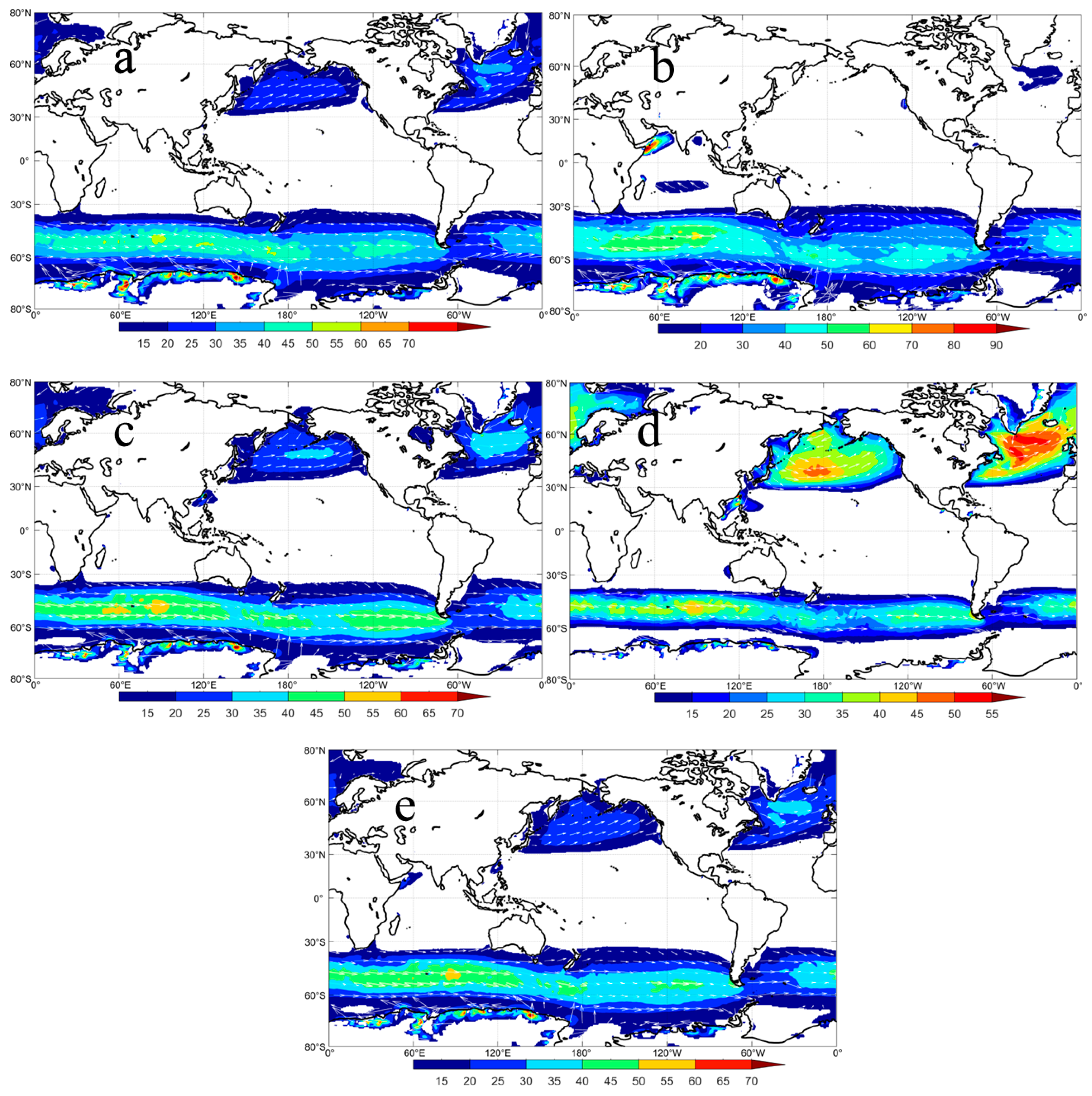
Calculate the global strong wind occurrence (SWO) above 11.7 m/s and determine the spatio–temporal distribution of SWO through climatological statistics, as shown in
Figure 1. Choose 1, 4, 7 and 10 as representative months for the four seasons.
In spring (
Figure 1a), the SWO extreme zone occurred in the westerlies of the Northern and Southern Hemispheres, with the highest value reaching 55% in the North Pacific and North Atlantic and only 45% to 50% in the westerlies of the Southern Ocean. In total, 30% of the area was in the Taiwan Strait and the South China Sea near China. The areas with frequent strong winds in the Southern Hemisphere have a band-like distribution. In summer (
Figure 1b), the extreme center in the Northern Hemisphere disappears or becomes weaker, while the extreme center in the Southern Hemisphere becomes stronger, revealing more than 50% of the area. In total, 90% of the area lies on the edge of Antarctica. In autumn (
Figure 1c), all extreme centers in the Northern Hemisphere disappear and areas with over 90% SWO are frequently affected by strong winds in the Arabian Sea. The SWO in the Southern Hemisphere continues to intensify with an extreme region of around 70%. In winter (
Figure 1d), a high-quality SWO area appears in the Northern Hemisphere westerlies, with only 35% of the high-quality area distributed in the North Pacific and North Atlantic. There are large areas of value in Taiwan, China, and the South China Sea. The intensity of high-value areas in the Southern Hemisphere decreases and the distribution area decreases. Annual average (
Figure 1e): The average annual distribution of SWO is similar to that in October. In total, 20 to 30% of westerly winds occur in the Northern Hemisphere. More than 20% of the area lies near Taiwan, China, China and the Arabian Sea. The Southern Hemisphere westerlies are banded and range between 15 and 45%, and 55% of the extreme value centers are in the southern Indian Ocean.
The weakest season for SWO in the Northern Hemisphere is summer, when Strong Winds are common in the Southern Hemisphere. The Arabian Sea is often exposed to strong winds in summer. In winter, SWO is strongest in the Northern Hemisphere, while SWO in the Southern Hemisphere becomes weaker and its range decreases.
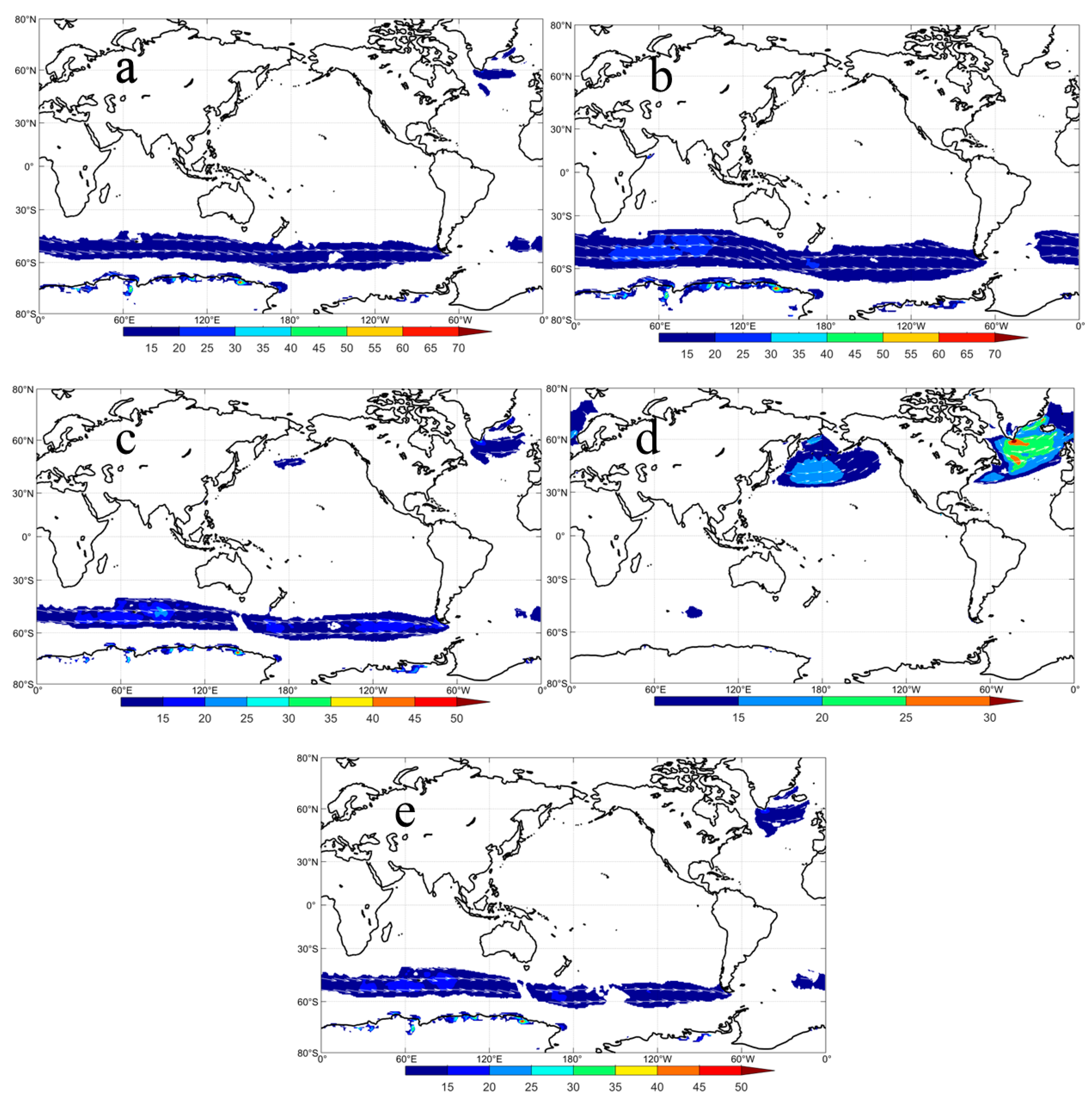
In analyzing the frequency of wind velocities exceeding 15 m/s, as depicted in
Figure 2, it is observed that the global prevalence of such wind speeds exhibits a general decline. Notably, even within the westerly zone of the Southern Ocean, characterized by typically robust wind velocities, the frequency remains below 20%. Higher frequency distributions are primarily concentrated in the Antarctic region, which further underscores the higher wind speeds prevalent in this area. It is particularly noteworthy that during the winter season in the Southern Ocean, occurrences of wind speeds above 15 m/s are sporadic. During this period, the Northern Hemisphere experiences more intense wind conditions, with over 30% of the affected regions being located in the southern Greenland North Atlantic area. Such a concentration of strong wind speeds in this central region is uncommon even in other seasons across the globe.
Figure 3 illustrates the frequency of wind velocities exceeding 20 m/s (
Figure 3a) on a global scale and those surpassing 25 m/s (
Figure 3b). It is evident that regions with wind speeds above 20 m/s are predominantly confined to the maritime areas surrounding Antarctica and in proximity to Greenland. Wind velocities exceeding 25 m/s are classified as extreme weather phenomena and are globally infrequent in their distribution.
4. Variation Trend
The Theil–Sen trend calculation was performed on SWO based on the variation trend, and the global trend of catastrophic wind volume growth was obtained by the MK significance test, as shown in
Figure 2. Choose 1, 4, 7 and 10 as representative months for the four seasons.
In January (
Figure 4a), the global SWO showed an increasing trend, with a significant increase of 0.1% per year in the Northwest Pacific and North Atlantic, an overall increase of 0.1%·yr
−1 in the Southern Hemisphere westerlies, and a significant increase of 0.1%·yr
−1 in the Northwest Pacific and North Atlantic. There was an increase of 0.2–0.3%·yr
−1 in the southern Indian Ocean, southern Australia and near South America. The increase in catastrophic winds in the above areas is not conducive to military activities abroad and the takeoff and landing of carrier aircrafts. In April (
Figure 4b), westerly winds in the Southern Hemisphere increase significantly, similar to January, but the increasing trend weakens. The growing regions in the Northern Hemisphere disappear. Near Antarctica, there is a decreasing area of −0.1%·yr
−1. Significant changes are observed in the Arabian Sea and the Southern Hemisphere westerlies in July (
Figure 4c). In the Arabian Sea, there is a clear decreasing trend of −0.3%·yr
−1 and in the westerly winds of the Southern Hemisphere, there is a clear increasing trend of 0.1~0.2%·yr
−1. In October (
Figure 4d), a waning center of −0.1 to −0.2%·yr
−1 appears near Baffin Gulf and the Aleutian Islands. The increasing trend in the Southern Hemisphere is increasing, with increasing centers of 0.1~0.3%·yr
−1 occurring in the Indian Ocean and the southern Atlantic.
5. Mechanism Analysis
5.1. Mechanism Analysis of the Correlation between Climate Index and SWO
To understand the correlation between SWO and key climate indices, a correlation analysis between both was conducted. The correlation between key climate indices and SWO is shown in
Figure 5.
The climate indices that significantly affect the SWO in the Southern Ocean are AAO and EP-NP and have a significant positive correlation reaching 0.5. There is a significant positive correlation between AAO and the Southern Ocean at 50° S to 65° S, with a band-like pattern. SWO, AAO and 40° S show a negative correlation of −0.3. The correlation between AAO and the Antarctic region is also inconsistent, with a significant negative correlation (−0.2 to −0.3) in southeast Antarctica and a sporadic positive correlation in southwest Antarctica. AAO is a phenomenon of atmospheric mass exchange between middle and high latitudes in the Southern Hemisphere, similar to a seesaw of atmospheric mass between middle and high latitudes. When the AAO is strong, the Southern Hemisphere deepens around the polar low and the westerly wind at mid to high latitudes strengthens [
54].
Previous studies [
55,
56] have found that due to the effects of global warming, the westerlies in the Southern Hemisphere are moving southward and their intensity is increasing, resulting in a significant positive correlation between the westerlies and AAO in the Southern Hemisphere, while a significant negative correlation is observed between them will be mid to low latitudes and AAO. EP-NP exhibits a long-range connectivity mechanism for SWO in the Southern Hemisphere, with a significant positive correlation between 0.3 and 0.5 in the Southern Hemisphere, especially in the waters near Antarctica. In the Northern Hemisphere, there is a significant negative correlation between −0.3 and −0.5. The EP-NP climate index is a model that reflects changes in spring, summer and autumn with three anomalous centers. Its positive phase features positive height anomalies over Alaska/Western Canada, while negative anomalies occur in the central North Pacific and eastern North America. When EP-NP is in the positive phase, the Pacific jet stream from East Asia to the Northeast Pacific moves southward and strengthens, resulting in an increase in the anticyclonic circulation over western North America, an increase in easterly winds and a decrease in westerly wind speeds, one decrease in SWO and a negative correlation.
The strengthening of the cyclonic circulation in the eastern part of North America is negatively correlated with a decrease in the SWO in the North Atlantic. AAO dominates the occurrence of SWO in the westerly zone of the Southern Hemisphere, while EP-NP dominates the enhancement in the Southern Hemisphere and the weakening in the Northern Hemisphere. The regions significantly correlated with AO are distributed across the Northwest Pacific, Greenland, North Atlantic and Mediterranean regions, with correlation coefficients ranging from −0.2 to −0.3. The positively correlated regions are distributed across the Norwegian peninsula, the New Territories and southern Greenland (0.2~0.3). Based on the AO changes, the SWO trend in the Northern Hemisphere can be determined. Additionally, a positive AO phase, deepening of the polar low pressure, strengthening of the pressure gradient, positive correlation in the Arctic and North Atlantic and negative correlation in mid-to-low latitudes can be observed.
ENSO is considered a representative climate phenomenon of global climate anomalies, with the Nino3.4 index and the SOI index representing different types of ENSO measurement. The Nino3.4 index and SWO show a correlation of 0.1~0.2 in the central Pacific, a negative correlation of −0.2 in western South America, a correlation of −0.15 near China and Australia and a correlation of 0.15 in South Australia. The correlation distribution of SOI is fundamentally opposite to the Nino3.4 index, with a negative correlation of −0.2 to −0.3 in the Pacific and southern Australia and a positive correlation of 0.2 in western South America, off the coast of China and in the Australian regions.
When PNA is positive, Pacific high pressure strengthens, increasing wind speeds in the mid latitudes of the Northern Hemisphere, and it is positively correlated with SWO in the mid latitudes of the Pacific. There is a negative correlation region of −0.2 in the Arctic Ocean.
By analyzing the correlation between key climate indices and the global SWO, changes in the SWO can be predicted based on changes in climate indices such as AAO and EP-NP, which have the strongest correlation with the SWO. If the above indices show positive reinforcement, one should beware of SWO sailing at 60° S in the Southern Ocean.
5.2. Contribution Rate of Climate Index to the SWO
In the previous section, the influence of key climate indices on SWO was analyzed and it was found that climate indices such as AAO and EP-NP have a strong correlation with SWO and have a significant influence. However, there is a lack of research on the contribution of climate indices to SWO. In this section, the contribution rate of key climate indices to the SWO is quantitatively calculated using Formulas (7) and (8). We calculated the contributions of climate indices such as AAO, EP-NP and AO to the frequency of strong winds in different seasons. The specific distribution of the index contribution rate is shown in the
Figure 6:
AAO showed a positive contribution to the frequency of strong winds in the Southern Hemisphere in all four seasons, with SON and DJF being the most significant. The strengthening of the AAO has resulted in a strong and southward shift of the western belt in the Southern Hemisphere, resulting in a positive contribution compared to the other two seasons. At the same time, with the strengthening of the western belt, the negative contribution of 40S has also shown an increasing trend, which is related to the strengthening of the AAO. It is worth noting that during the SON season, the Western Pacific region has a contribution rate of −40% and AAO shows a negative weakening trend in the frequency of strong winds in the Western Pacific.
The significant contribution areas of EP-NP are concentrated near North America, with positive contribution areas occurring in the northern Canadian Archipelago during the MAM and DJF seasons and significant negative contribution areas occurring in the eastern Pacific. EP-NP shows a weaker trend in the frequency of strong winds in this area with a reduction contribution of −50%. The Indian Ocean has a 30% contribution rate during the MAM season, and the EP-NP index has a 30% contribution rate to the frequency of strong winds in this area.
The contribution of AO index to the frequency of strong winds is concentrated in the Arctic Ocean and the North Atlantic region, which shows a positive contribution and promotes the frequency of strong winds in the Arctic Ocean region. The AO makes the most significant positive contribution in the Atlantic region during the DJF season. JJA is the largest contributor to the North American region, while MAM and SON are the largest contributors to the waters of northern Russia. AO contributes negatively to the Atlantic region only in winter and spring, reaching over −40%.
6. Discussion
AAO has a high contribution in the Southern Ocean, primarily because the AAO index represents the atmospheric mass exchange between mid and high latitudes in the Southern Ocean. When AAO is in a positive phase, mid-latitude pressure in the Southern Hemisphere increases, high-latitude pressure decreases, and the westerly jet becomes stronger and moves toward the South Pole, showing a strong positive correlation with the western belt. At the same time, a negative correlation area appears north of 40° S [
57]. In the fall and winter seasons of the Northern Hemisphere, the strengthening of the AAO leads to the strengthening and southward shift of the westerly winds, showing a significant positive correlation and positive contribution range in the fall and winter seasons. The positive phase of the Antarctic Oscillation is characterized by the occurrence of westerly wind anomalies across the mid to high latitudes of the Northern Hemisphere, concomitant with the emergence of easterly wind anomalies within the mid to low latitudinal zones.
EP-NP is a climate pattern that occurs primarily between spring and fall. There are three main anomaly centers. When EP-NP is in a positive phase, overpressure anomalies typically occur in Alaska and western Canada, while negative anomalies occur in the North Pacific and eastern North America. The reasons for the negative correlation between the Pacific and Atlantic are not the same. The Pacific is influenced by the pressure gradient force between the atmospheric high pressure in Alaska and western Canada and the atmospheric low pressure in the North Atlantic. The generation of easterly winds weakens the westerly circulation, while the southward movement of the North Pacific jet from East Asia to the eastern North Pacific results in a significant negative correlation in the North Pacific. The negative correlation in the Atlantic is due to the increased cyclonic circulation in this area, which leads to a reduction in the frequency of strong winds and represents a negative correlation.
AO has shown great influence in the Northern Hemisphere and represents an inverse relationship between the atmospheric pressure in the Arctic and the pressure in the mid latitudes of the Northern Hemisphere. The positive phase of AO corresponds to the lower atmospheric pressure in the Arctic, where the cold jet of the polar vortex strengthens around the Arctic and suppresses the southward spread of cold air from the polar vortex and promotes the occurrence of strong wind frequencies [
58]. In instances where the Antarctic Oscillation (AO) Index exhibits negative anomalous variations, there is an expansion of the polar vortex domain, accompanied by an intensification of cold air dynamics. Concurrently, the mid-latitude meridional circulation experiences a weakening trend, while the meridional circulation in other regions is enhanced, fostering a more vigorous exchange of cold and warm air masses. This scenario is marked by the southward incursion of polar cold air into the mid latitudes, culminating in unusual cold weather phenomena across Eurasia [
59].
SOI indicates the pressure difference between the eastern and western Pacific, which represents the monthly SLP anomaly between Tahiti and Darwin. In a positive phase, the subtropical high pressure in the southeast Pacific strengthens, which has a beneficial effect on the westerly wind and promotes the development of strong winds [
35]. The eastern region of Australia south of the equator and the Pacific Ocean in the eastern East China Sea are characterized by cyclones in the upper layers and anticyclones in the lower layers. The lower layers of the Eastern Pacific in the equatorial region are characterized by centers of divergence, while the upper layers are characterized by centers of convergence, which favor subsidence and have negative effects on trade winds [
60,
61].
7. Conclusions
This study uses the frequency of global wind speeds above 11.7 m/s as an assessment index of catastrophic winds, analyzes the spatiotemporal characteristics and development trends of SWO, and analyzes the correlation between key climate indices and global SWO and the contribution of key climate indices to it.
1. The global SWO occurs in the Southern Ocean (30~50%), the North Atlantic (20~30%), the North Pacific (20%), near Taiwan, China (10~20%), and the Arabian Sea (10~20%). Among them, the SWO in the Arabian Sea region is dominated by summer, and the SWO in spring, autumn and winter in the North Atlantic and North Pacific is reflected. The strong winds occurrence in the Southern Hemisphere is reflected in all four seasons, with no obvious dominant season. The summer SWO is the strongest season in the world, with the greatest impact of catastrophic winds. In winter, SWO is at its weakest all year round, while SWO is common in the North Pacific, which can easily have fatal effects on ship navigation and carrier aircraft takeoff and landing.
2. The variation trend of SWO is strongest in the Southern Ocean, with the strongest growth trend (0.15~0.2%·yr−1) in the Southern Indian Ocean and the Southern Indian Ocean. The declining regions are distributed near the Arabian Sea and the Bay of Bengal, reaching −0.05%·yr−1. The increasing trend of SWO in the Southern Ocean is reflected in all four seasons.
3. The climate indexes with the strongest correlation with global SWO are AAO and EP-NP, which can reach between −0.5 and 0.5, and are positively correlated with the Southern Ocean 60° S. Climate indexes related to the Indian Ocean include EP-NP (positively correlated) and WP (positively correlated). Related to the Pacific are AO (negative correlation), EP-NP (negative correlation), Nino3.4 (positive correlation), PNA (positive correlation), SOI (negative correlation) and WP (negative positive correlation). The Climate indexes that are correlated with SWO in the Atlantic include AO (negative correlation), EP-NP (negative correlation), NAO (positive negative correlation), SOI (positive correlation) and WP (negative correlation).
4. Based on the climate index and the global SWO, this article determines the contribution rate of the climate index to the SWO, which is divided into facilitating contribution and inhibiting contribution. AAO has a significant contribution to SWO at 60° S, while its contribution to SWO is inhibited at 40° S and in southeast Antarctica. Climate indices related to the Indian Ocean include EP-NP (Promotion) and WP (Promotion). Related to the Pacific are AO (inhibition), EP-NP (inhibition), Nino3.4 (promotion), PNA (promotion), SOI (inhibition) and WP (inhibition promotion). Climate indices correlated with SWO in the Atlantic include AO (inhibition), EP-NP (inhibition), NAO (promotion inhibition), SOI (promotion) and WP (inhibition).


