1. Introduction
As we all know, more than 70 percent of the earth’s surface is covered with oceans that are full of future energies, thus countries are increasingly paying more attention onto the exploration of marine resources. Autonomous underwater vehicles (AUVs), as a kind of exploring equipment that could dive several hundred meters to conduct research activities without operators, play an increasingly important role in the marine development domain [
1]. With the development of artificial intelligence technology and manufacturing technology, AUVs have transformed from semi-intelligent, huge and heavy equipment with economic shortcomings to highly autonomous, small and flexible tools with relatively low cost, which makes it more reliable and easier to conduct ocean research activities [
2,
3,
4].
Nowadays, in all kinds of underwater tasks, both civilian and military, such as deep sea inspections, seabed topography surveys, seabed target search, oceanographic mapping, mine detection and neutralization [
5,
6,
7,
8,
9,
10], an AUV can find its own specific position. Terrain following is one of the most significant methods to efficiently carry out the missions mentioned above [
11,
12]. In order to obtain high-resolution seabed topography and surface details from various sensors, an AUV has to descend to a low altitude and steadily maintain a specified height, although topographic data are usually not known in advance [
13,
14]. Additionally, an AUV needs to be able to avoid collision danger, even though the terrain may be rough sometimes. As a result, with the sharp increase in accurate and efficient tracking requirements, a key problem arises in the terrain-following-based task: how can we track a terrain surface with high precision and good safety under sensing instruments with limited capabilities [
15]? Therefore, various approaches have been proposed for seabed terrain tracking in recent years.
Regarding the path planning problem of AUV terrain tracking, Hongli Xu et al. proposed a bounded ridge-based trajectory planning algorithm (RA*) for an AUV to cruise near-bottom with a safety map based on a spherical structure [
16]. Kangsoo Kim et al. [
15,
17] discussed an altitude-based steep terrain tracking method with consideration of possible collisions because of altitude overestimation or loss of bottom lock. Then, waypoint-based motion control was carried out to realize pseudo-terrain, followed by a procedure to guarantee safety. In reference [
18], the authors proposed a safe near-bottom planning method based on the spline curve of along-track terrain, and the constraints of a dynamic model of an AUV are also satisfied according to the curvature designed. To obtain along-track terrain data simply and efficiently, the authors of [
19] presented a method regarding terrain fitting with Doppler velocity log (DVL) data and carried out altitude control with an observer to estimate seafloor gradient. In addition, in Ref. [
20], the authors further proposed seafloor geometry approximation with an altitude rate of change and fine/coarse contouring with an adaptive adjustment of the surge velocity. Even though the research results of [
19,
20] were about ROVs, sensors and strategies were also feasible for AUV platforms. Ref. [
21] designed a robust NMPC scheme to steer an AUV to the desired trajectory inside a constrained and dynamic workspace, whose knowledge is constantly updated online via the vehicle’s onboard sensors, and obstacle avoidance is guaranteed by the online generation of a collision-free trajectory-tracking path. A tube MPC scheme was addressed in [
22] for continuous-time nonlinear systems that were subjected to bounded disturbances; the actual system was divided into an error system and a nominal system, and the actual trajectory was in the sets centered along the nominal trajectory. The authors of [
23] proposed a method of path planning for an AUV’s seabed terrain-matching navigation based on an A-star algorithm. It analyzed an area’s matching performance by mainly using terrain entropy and terrain variance entropy, and the search length and dynamic matching algorithms were presented to reduce the calculation burden. Furtermore, an online path planning methodology was addressed in [
24] for terrain-aided navigation of AUVs, which applied a particle filter to obtain AUVs’ localization and set commands to AUVs. This methodology’s feasibility and maneuvering performance were finally proven through simulation experiments.
Besides seafloor approximation and path planning, another key component of terrain following is an appropriate control methodology. Steenson et al. [
25] proposed a model predictive control method for depth control through linearization of the dynamic model and successfully enabled the AUV to follow the terrain within 1 m in lake experiments with hovering and flight-style modes. The authors of [
12] presented a nonlinear model predictive controller with a combination of tracking differentiator (TD) and long short-term memory (LSTM) in order to improve the control accuracy with low computational costs. Yan et al. [
26] addressed the bottom-following problem of AUVs using integral terminal sliding mode control (ITSMC), which guarantees an exponential vertical plane path following, with a tolerance of parameter perturbations. Gao in [
27] proposed an improved finite-time disturbance observer-based finite-time control (IFTDO-FTC) scheme for implementing the exact bottom-following of a biomimetic underwater vehicle (BUV) with the consideration of saturation and uncertainties based on the integral terminal sliding mode control framework. Tao Liu et al. [
28] designed a deep reinforcement learning controller for vectored thruster AUVs, which only used the sensors’ measurements as inputs and outputs continuous control actions; thus, the AUV’s accurate mathematical model is unnecessary. Another continuous control strategy under deep learning frameworks was proposed by the authors of [
29] using a deep interactive reinforcement learning method based on the Deep Deterministic Policy Gradient (DDPG). Its experimental simulation results showed that this strategy could increase the precision of an AUV’s path following while simultaneously reducing time consumption. In [
30], the authors designed a kinematics controller and a dynamic controller, the kinematics controller was designed based on a model predictive control (MPC) that took wave disturbances into account, and the dynamic controller was designed based on adaptive dynamical sliding mode control (ADSMC) that could reduce errors resulting from model uncertainties.
As a matter of fact, many trajectory tracking methods can be adopted for the terrain-following control of AUVs [
31]. For example, due to practical simplicity and stability, PID-based methods are still preferred by industrial and commercial fields for many real-life marine operations and control [
32,
33]. In [
34], performances of PD-based non-model control schemes were compared with model-based ones. Other than the PID method, the authors of [
35] proposed to combine the advantages of sliding mode control (SMC) and back-stepping control, aiming at uncertainties and disturbances of AUV operations in an ocean environment. Qiao et al. in [
36] designed an adaptive sliding mode control method for AUV trajectory tracking, which handles both model uncertainties and external disturbances with fast convergence performance.
Based on the above discussions and the purpose of this paper, the main contributions of this paper are focused on two aspects that can be summarized below:
Navigating in an unknown environment autonomously to execute terrain-following tasks. In response to this target, a terrain-aided navigation strategy is proposed, by which the modeling of data from onboard sonar devices is accomplished for reliable height and slope estimation. Note that as a preferred and economical option for an altitude-measuring device, multiple single-beam echo sounders are equipped in the vehicle and set in different directions, which forbids the phenomenon of bottom lock loss in rough terrain scenarios.
Terrain tracking control architecture with the decoupled mathematical model. The algorithm constructed in this paper converts three-dimensional (3D) terrain following into a joint control of motions in horizontal and vertical planes. Specifically, in the horizontal plane, the AUV tracks the desired 2D waypoints. Meanwhile, it adopts a back-stepping technique to establish a depth controller that allows us to follow the surface of the terrain at a fixed altitude near the seafloor without collisions.
To better compare the proposed method with existing ones,
Table 1 illustrates the characteristics of this paper. As shown, neither sensor configuration nor the control method adopted in this paper is the most advanced, but balance is acquired with the proper choice of relatively simple sensors combined with a slope-based terrain construction strategy, which makes the methodology discussed here capable of handling steep terrain variations that are not applicable for certain methods in the table.
The remainder of the paper is organized as follows.
Section 2 presents the mathematical model of an AUV and the underlying bottom construction method for terrain following with simple beam-based data. Then,
Section 3 discusses the model-based back-stepping controller design and delivers the stability proofs in vertical plane for terrain tracking. Simulation results of applying the proposed terrain-following strategy to an AUV in a complex seafloor environment are provided in
Section 4. Finally,
Section 5 concludes this paper.
2. Problem Formulation
The problem of seafloor terrain tracking is essentially a complex process of online terrain perception, fixed height navigation and obstacle avoidance. To design an effective seafloor terrain tracking strategy, two requirements must be met. The first requirement is to comprehensively utilize sonar configuration and detection information to realize terrain perception. The other one is to achieve fixed-altitude navigation and obstacle avoidance. As shown in
Figure 1, the distance between the AUV and seafloor terrain is defined as
h, and the distance between AUV and sea level is defined as
z. Obviously, there is a risk of collision when an AUV is operating near the seafloor. Therefore, terrain tracking with a fixed altitude value is necessary to avoid obstacles during the tracking. But practically, topographic characteristics of the rugged seafloor are hard to predict in advance for engineering applications and online prediction encounters difficulties in reliability and financial cost.
To better formulate the terrain tracking problem, a mathematical model of an AUV is constructed with the kinematic part and dynamic part in the following sections in order to design proper controllers. In addition, to navigate in-vertical plane safely during the tracking process, a seafloor feature extraction method is proposed with consideration of the different types of seabed topography, including six different situations in
Section 2.2 with limited sensor data requirements for practical feasibility.
2.1. Kinematics and Dynamics
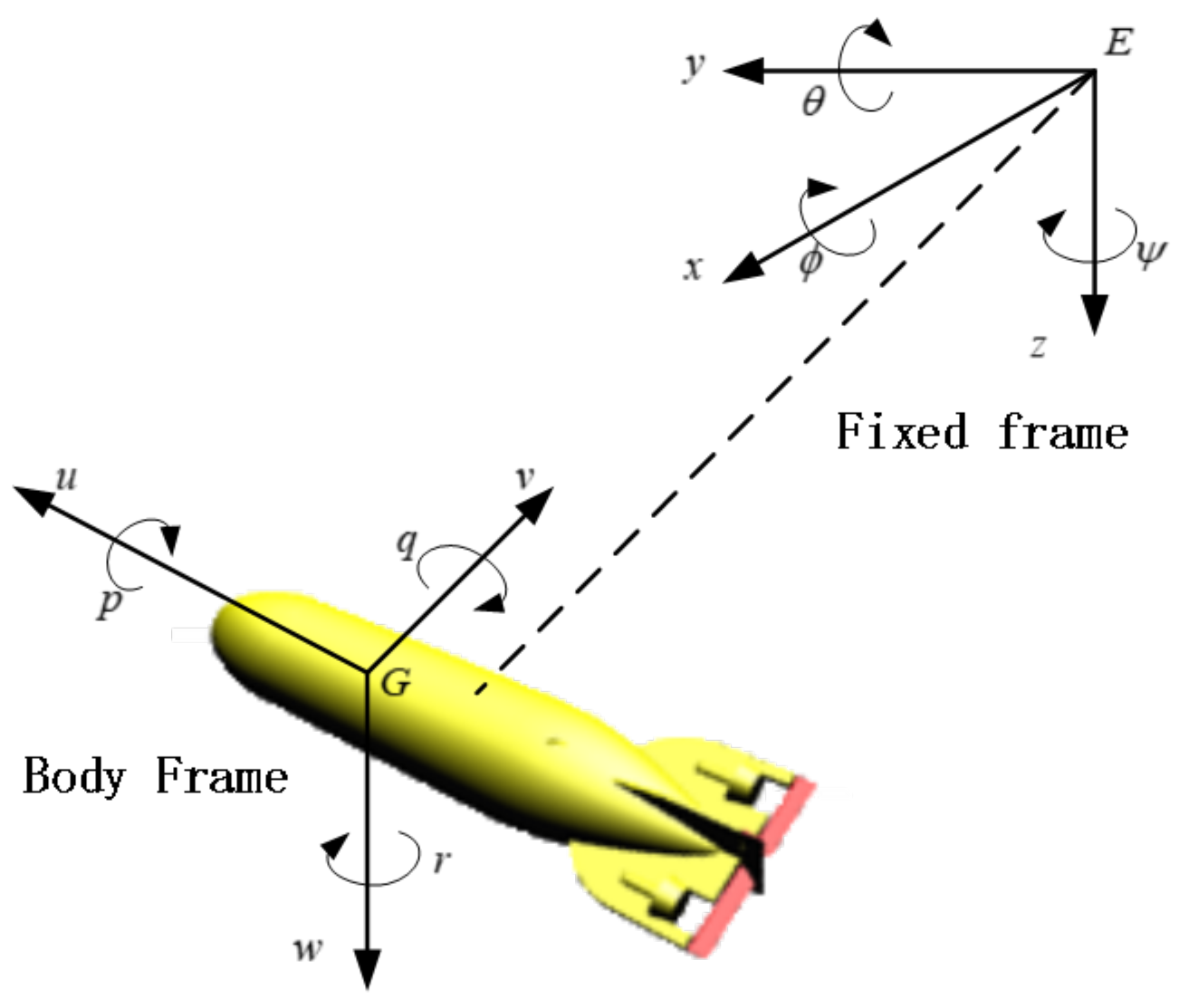
The coordinate frames adopted in this paper are illustrated in
Figure 2, including the position, attitude, velocity and angular velocity variables of an AUV. In general, a 6-degree-of-freedom (DOF) mathematical model of an AUV is described by several nonlinear and strong coupled differential equations, as presented in [
37]. Ignoring the relatively stable roll dynamic of the vehicle and considering its symmetric structure, the vertical-plane dynamics are presented for the terrain-following scenario and altitude-keeping controller design.
First of all, a 5-DOF kinematic model without consideration of roll is depicted below, representing the transformation between the body frame and the fixed frame:
where
x,
y and
z are surge, sway and heave displacements, while
and
represent pitch and yaw angles in the fixed frame, respectively.
u,
v,
w,
q and
r are linear and angular velocities in surge, sway, heave, pitch and yaw directions of the body frame. In addition, the corresponding dynamic model is shown as Equation (
2), defined in body frame:
where
m represents the mass of the AUV and the hydrodynamic-added mass terms are defined as
,
,
,
,
, where
is the moment of inertia about the
y axis and
is the moment of inertia about the
z axis. For damping items, we have
,
,
,
,
, respectively.
Furthermore, static hydrodynamic and control surface coefficients are defined as , , , , respectively, with and as centers of gravity and buoyancy, and W and B as the weight and buoyant force of the vehicle. In addition, , and are control inputs provided by thrusters and horizontal and vertical rudders.
Taking advantage of the design of orthogonal rudders and symmetric hull, Equations (
1) and (
2) can be divided into two non-interacting models for horizontal and vertical planes without loss of generality. Then, the equations of vertical motion can be extracted from the 5-DOF mathematical model in both kinematic and dynamic domains, as shown below:
and
Based on hydrodynamic simulation and practical experiments on the depth control of a vehicle, it can be concluded that vertical velocity
w is much smaller compared to longitudinal velocity
u for AUVs with near-cylinder shapes and can be eliminated. Therefore, Equation (
3) is further reduced to
2.2. Terrain Feature Extraction
In terrain-following missions, in order to obtain real-time altitude data above the terrain surface, only three single-beam echo sounders with certain installation angles (one forward facing, one downward facing, and one backward facing) are mounted on the vehicle in this paper to map the true seafloor topography. Then, a slope-based method is proposed to realize local environmental information extraction and real-time altitude command generation to execute terrain-following tasks.
The distance from the vehicle to the seabed datum and a height correction value induced by topographic variations on the seafloor are generated as measurements described below:
where
h is the current vertical height of the vehicle relative to the terrain surface;
d is the relative range measured by sonar and
indicates the installation angle of an echo sounder transducer. Define the angles between three single-beam echo sounder directions and the positive x-axis of the body-fixed reference frame as
and
, respectively, and it can be obtained that
and
with
for
. Then, the current altitude measurement
h can be acquired based on Equation (
5).
Due to complex seafloor features such as canyons, seamounts and hydrothermal vents, six typical and representative cases are taken into account for extracting local features and generating real-time height command corrections, as shown in
Figure 3.
In the above figure, points
,
,
represent detecting positions of three single-beam echo sounders in vertical plane, where
and
can be calculated from
and
, respectively, as below for
:
In addition, define
,
and
as slopes of straight lines
,
and
, respectively. Based on illustrations in
Figure 3, it can be easily presented that
As a result, the method for describing terrain features corresponding to typical topographies can be presented as follows, along with the calculation of the height correction value.
Case 1. Steep uphill. When , it indicates that the terrain is uphill, and the slope is rising. The uphill portion poses a considerable risk of collision impact on the AUV. To enable the AUV to conquer steep uphill terrains, a higher slope parameter is used to generate the correction of height concerning altitude changes. Thus, it is defined as , where T is the sampling period.
Case 2. Small-scale sag. When , one possibility is that the AUV is trapped in a relatively small but V-shaped underwater canyon. Considering factors such as track quality, vehicle stability and safety, techniques to smooth the terrain should be considered and the terrain surface with slope is suitable to be chosen as the tracking objective. The altitude change value is adopted as .
Case 3. Steep downhill. When , it implies that the AUV is moving down an increasingly steep hill with a low altitude. To prioritize vehicle safety, a solution to remedy the situation is to follow the trend of gentle terrain gradient. Although tracking the steeper part of the terrain is an alternative solution, overshoot may be produced when the vehicle arrives at the end of the downhill route due to inertia and delays. In light of these concerns, is chosen in this case.
Case 4. Small-scale uplift. When , similar to the analysis process in case 2, the small uplift can be ignored in order to keep the tracking process stable. A compromise strategy for terrain following is adopted as .
Case 5. Gentle uphill. When , it can be observed that the terrain offers a gentle slope. Note that the underactuation of a vehicle leads to constraints on its depth adjustment capability. Concerning this problem, the higher slope is utilized to generate a new value for the altitude, i.e., , which allows the vehicle to quickly climb the uphill section at a specified vertical distance above the terrain.
Case 6. Gentle downhill. When , the vehicle is facing a gentle downhill. To ensure the safety of the vehicle, an altitude command is given as , although tracking precision has to be sacrificed to some degree.
By integrating strategies gained in the above-discussed cases, it can be concluded that in different scenarios, the definition of
can be defined as
Furthermore, define the altitude tracking error
as
, where
is the desired (reference) vertical distance between the vehicle and the sea bottom, and
is a vertical profile command signal. Note that
will usually be converted into a depth error counterpart of the AUV as in
Figure 1, and then a depth controller can be in charge of the terrain-following control in the following controller design.
3. Terrain-Following Controller Design
A terrain-following mission has two purposes: On the one hand, it is necessary for the mission to maintain a predetermined height above the seafloor in order to ensure the performance of the sonar. On the other hand, it is also necessary for the mission to be able to adjust the depth quickly enough so that substantial threats can be dealt with if steep-sided terrain features are present. In order to achieve the control purpose, a back-stepping control strategy is proposed in this section based on a multi-oriented observation of terrain characteristics in order to maintain a constant height above the seafloor. A transformation between the altitude above the seafloor and the depth below the sea level is established so as to convert terrain-following into a traditional depth tracking control problem, which is finally implemented by adjusting horizontal rudder angles.
Define
as the along-track depth error, where
represents the desired depth of the vehicle for sailing and
z denotes the current depth obtained from a depth meter. It can easily be understood that
. Then, the control surface deflection angle is decided by
where
,
,
,
and
is the upper bound of velocity
u. According to the problem formulation of
Section 2, the main result of this paper is given in the following theorem.
Theorem 1. Consider an AUV with kinematics Equation (
1)
and dynamics Equation (
4)
. If the terrain-following controller is designed as (
10)
, then the equilibrium point of the underlying system is globally asymptotically stable. Proof of Theorem 1. Construct a Lyapunov function as
Taking the derivative of
along with the trajectory of
yields
Then, define the virtual control input and the tracking error of pitch angle as
and
, respectively. By taking the case where the desired depth signal is a step function as an example, there holds
. Then, it follows from Equation (
12) that
In addition, due to
and
for
, it can be concluded that
Consequently, the second Lyapunov function can be constructed as
and the derivative of
leads to the following equation:
Let
and based on (
16), the following can be obtained:
Define the virtual control input and the tracking error of pitch angular velocity as
and
. Meanwhile, the function Equation (
17) is reconstructed as
where
is ensured according to parameters adopted in Equation (
10). Then, we can construct the third Lyapunov function as follows:
Differentiating the expression of
gives
From Equation (
10), we have
By integrating (
21) into (
20), one arrives at the following inequality:
□
As a result, it can be concluded that the back-stepping depth controller designed in this section ensures that all the terrain-following errors converge to zero. The proof is complete.
4. Simulation Results
In order to better verify the proposed method, a comprehensive two-dimensional vertical terrain is established to simulate the influence of different parameters such as the speed of the AUV and installation angles of the sonars on the method. Then, a random three-dimensional terrain is built by superimposing several Gaussian formulas and comparing the results with the typical distribution formula as follows, to confirm the effect of the design strategy. Then, a simulated seafloor terrain can be constructed with random parameters and an along-track profile sample-generated depth command can be calculated according to Equation (
9).
Simulations are carried out in a C/C++ environment and visualizations of data are carried out with Origin from OriginLab. To realize numerical integration according to the Runge–Kutta algorithm, major parameters of the AUV mathematical model are listed below in
Table 2. Due to the calculating advantages of C/C++, the frequency of dynamic model integration is chosen as 50 Hz and the control frequency is 2 Hz with consideration of sonar property in practice. According to Equation (
10) and model parameters in
Table 2, the control parameters were chosen as
,
,
,
during the simulation.
4.1. Tracking Performance with Different AUV Speeds
In the AUV terrain-following mission, different speeds will affect tracking performance. According to the formula , it can be noticed that the altitude error is affected by the speed of the platform, so the vehicle is simulated at different speeds to better illustrate this problem.
Through comparing the tracking effects in three different cases shown in
Figure 4,
Figure 5 and
Figure 6, it can be noticed that accurate terrain tracking can be achieved at three different speeds when tracking gentle terrain. In the sudden change part of the terrain, the terrain tracking error is the largest when the speed is 3 m/s, which also reflects the practical property. However, even though depth error increases with the speed of the AUV, the converge process is quick enough based on the designed controller with a maximum error of less than 2.5 m, which can guarantee the safety of the platform. The simulation results are presented below.
4.2. Tracking Performance with Different Installation Angles
From Equation (
6), it is apparent that the installation angle of a single-beam sonar will have an impact on the results of different topography ranges. As a result, the height error of the terrain tracking control is affected. When the vehicle is moving at a specific speed, the seafloor points detected by sonars with various installation angles are dissimilar. Consequently, the
k values obtained onboard during control are also different, which in turn affects the performance of the depth controller for tracking performance.
According to the simulation results shown in
Figure 7,
Figure 8,
Figure 9 and
Figure 10, it can be inferred that within the research scope, four groups of different sonar installation configurations can all achieve terrain tracking with satisfactory performance. From the perspective of terrain tracking effect, altitude tracking error and pitch angle change, the changes are consistent across all four cases, and there is no discernible difference with respect to the same terrain.
However, upon comparing the changes of rudder angle command in four cases, it can be inferred that the internal adjustment process of the horizontal rudder is not that similar. When the forward sonar angle remains constant, the rudder angle changes more frequently as the backward sonar angle increases. Similarly, when the angle of the backward sonar is constant, the steering angle adjustment curve becomes stronger as the angle of the forward sonar increases. It can be concluded that good terrain tracking can be achieved by using the proposed strategy under four different installation angles simulated. In order to make the rudder angle change to be relatively gentle, the installation angle of the two sonars can be reduced under the premise of ensuring the tracking effect.
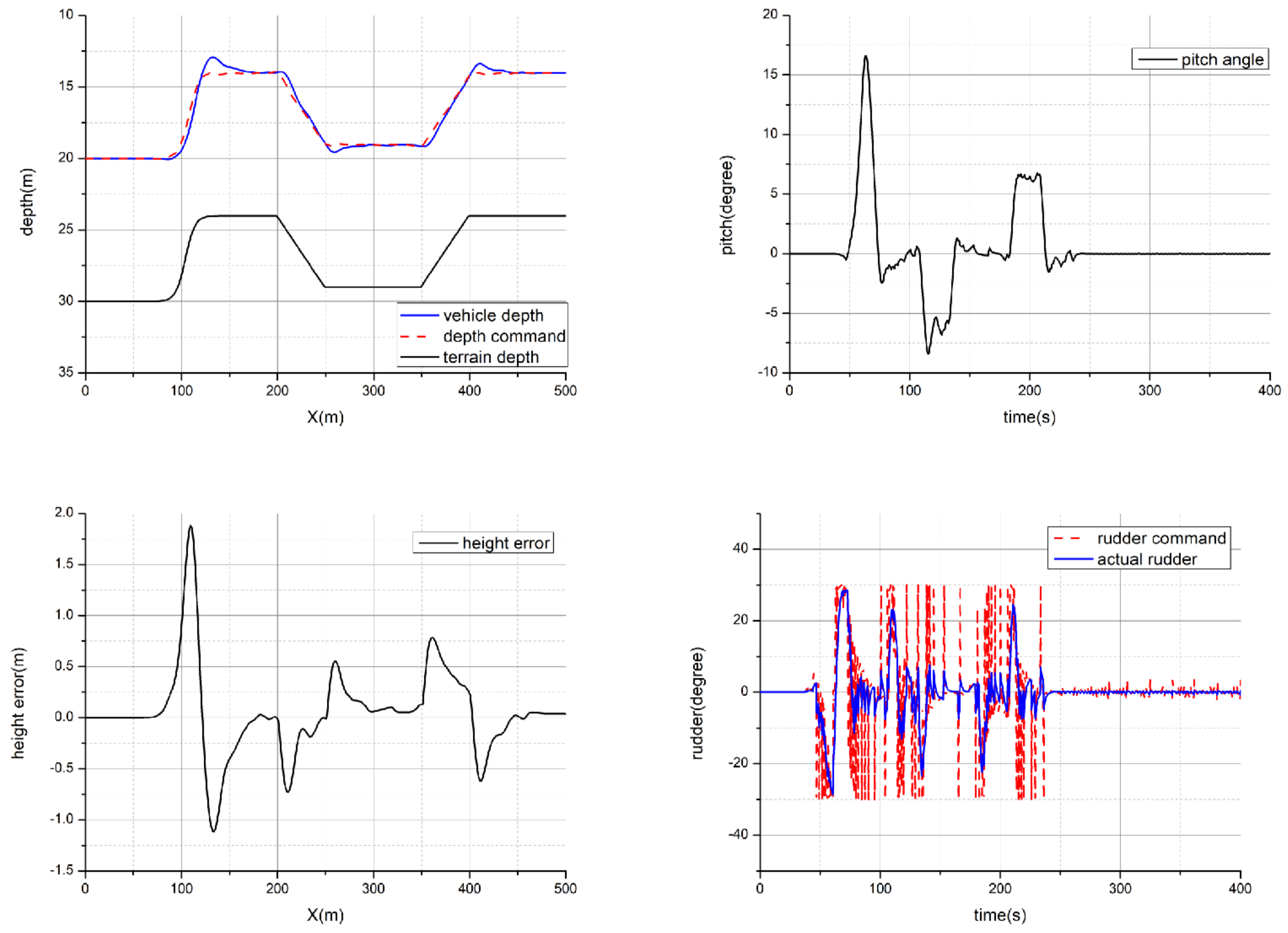
4.3. Three-Dimensional Terrain-Following Simulation
To further demonstrate the feasibility of the method proposed in this paper under a more complex environment, terrain-following simulation regarding three-dimensional seafloor constructed with seven Gaussian functions is carried out. Parameters of Gaussian functions adopted in the simulation are listed in
Table 3. The initial position of the AUV is set at
with a height of 40 m, and the final target position is
. During the simulation, the AUV surge velocity is set as 2 m/s and the terrain tracking results are shown in
Figure 11.
It is worth noting that even though the path of an AUV has encountered peaks and valleys in the terrain, an AUV has completed the desired path safely. The height error and pitch angle curves during the tracking process are presented as
Figure 12 and
Figure 13 below, with the largest height error being 1.11 m due to drastic changes in terrain. Based on the simulation, it can be concluded that the methodology presented in this paper is capable of tracking complex terrain with a simple sensor configuration and can guarantee the safety of platform effectively.


