
Sediment Thickness Model of Andalusia’s Nearshore and Coastal Inland Topography

 ,
, 
 ,
,
Abstract
:
1. Introduction
2. Background and Ancillary Data Used
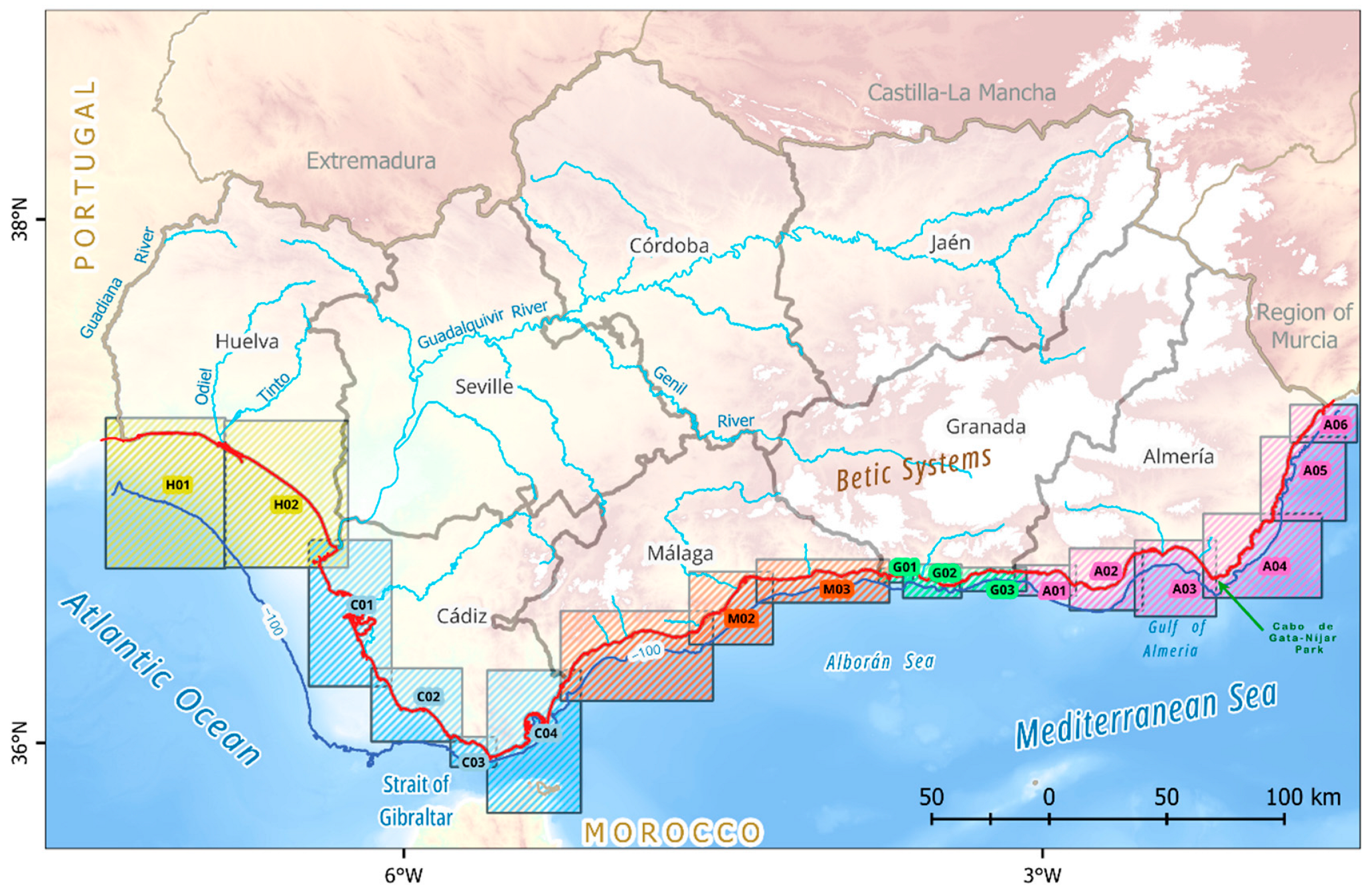
2.1. Study Area
2.2. Data Input
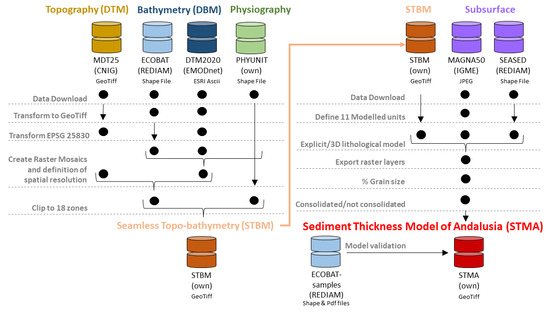
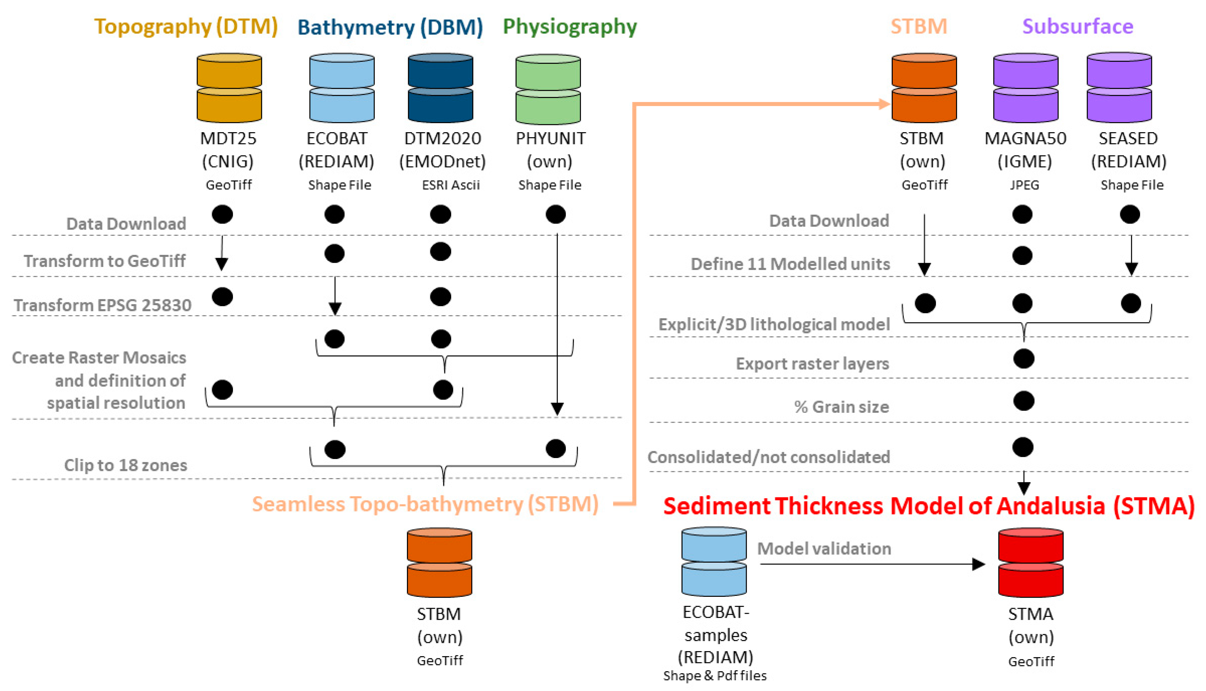
- One Seamless Topo-bathymetry model (STBM) for each zone. This dataset is a raster mosaic divided by 18 zones (see Figure 1). Each zone was compiled by mixing topographic and bathymetry data and filling in and interpolating the gap areas. The geodata sources in this dataset were:
- Topography: the elevation was obtained from the Digital Terrain Model (DTM) with a 25 m grid pitch obtained by interpolation of 5 m-cell size DTM from LiDAR 2014–2015 flights, in Spanish called MDT25 and distributed by the Spanish National Center for Geographic Information (CNIG, in Spanish Centro Nacional de Información Geográfica) [30].
- Bathymetry: For the seabed, two main datasets were collected. In shallow water, several Eco bathymetries (ECOBAT) were downloaded in ESRI shape format from the Andalusian environmental network website called REDIAM (in Spanish, REd De Información AMbiental de Andalucía) [31]. They were mapped with bathymetric contours at 1:1000 (Cádiz, Granada, and Almería) and 1: 5000 (Málaga) scales between 2008–2012 [32]. They cover the whole Andalusia coastline (<100 m depth), except the Huelva shoreline, and were interpolated to obtain a continuous GeoTiff format. In Huelva and deep waters, the F3 and F4 tiles from the DTM 2020 product by EMODnet Digital Bathymetry were collected [33].
- Physiographic zones: Due to the extension of the coast and its wide geomorphology, 17 (18 at the end) physiographic zones were defined. They were based on the orientation of the coastline, the shape of the continental shelf, river intersections, headlands, the main sediment type, and the level of influence from atmospheric and maritime weathering agents.
- Coastline: The topographic and bathymetric datasets were joined using an additional vectorial layer as the limit between land and sea. The layer was downloaded for each province from the REDIAM website [34].
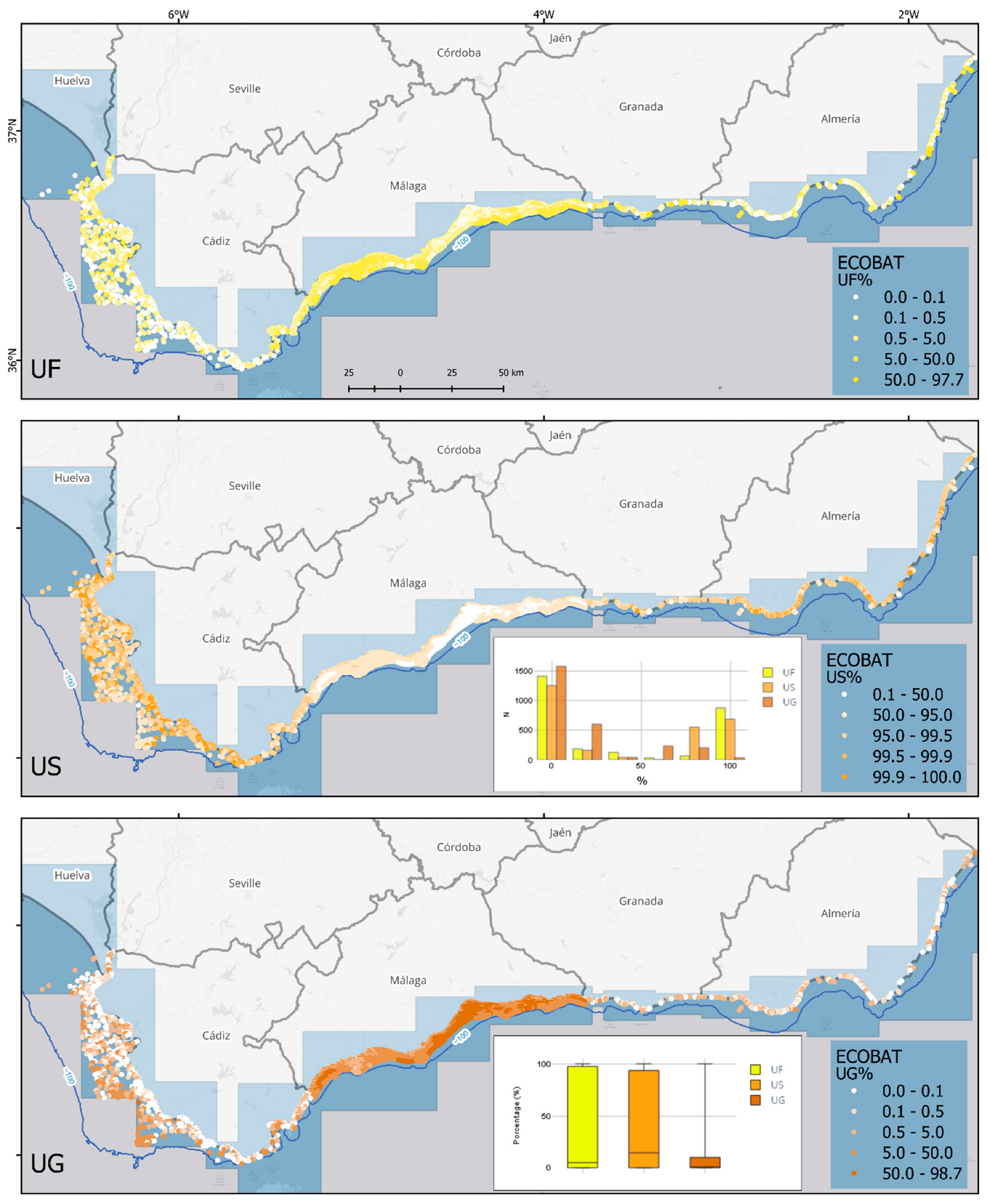
- Seabed sediment samples and Granulometric curves: During ECOBAT, field surveys obtained more than 4500 samples of seabed sediments in the study area [32]. This information is used to control the quality of the model. The percentage of fine (<0.063 mm), sand (>0.063 mm and <2 mm), and gravel (>2 mm) material, according to the sediment type division in our STM for each point, was obtained from the granulometric curves.
- Subsurface. This dataset is composed of two main subsets:
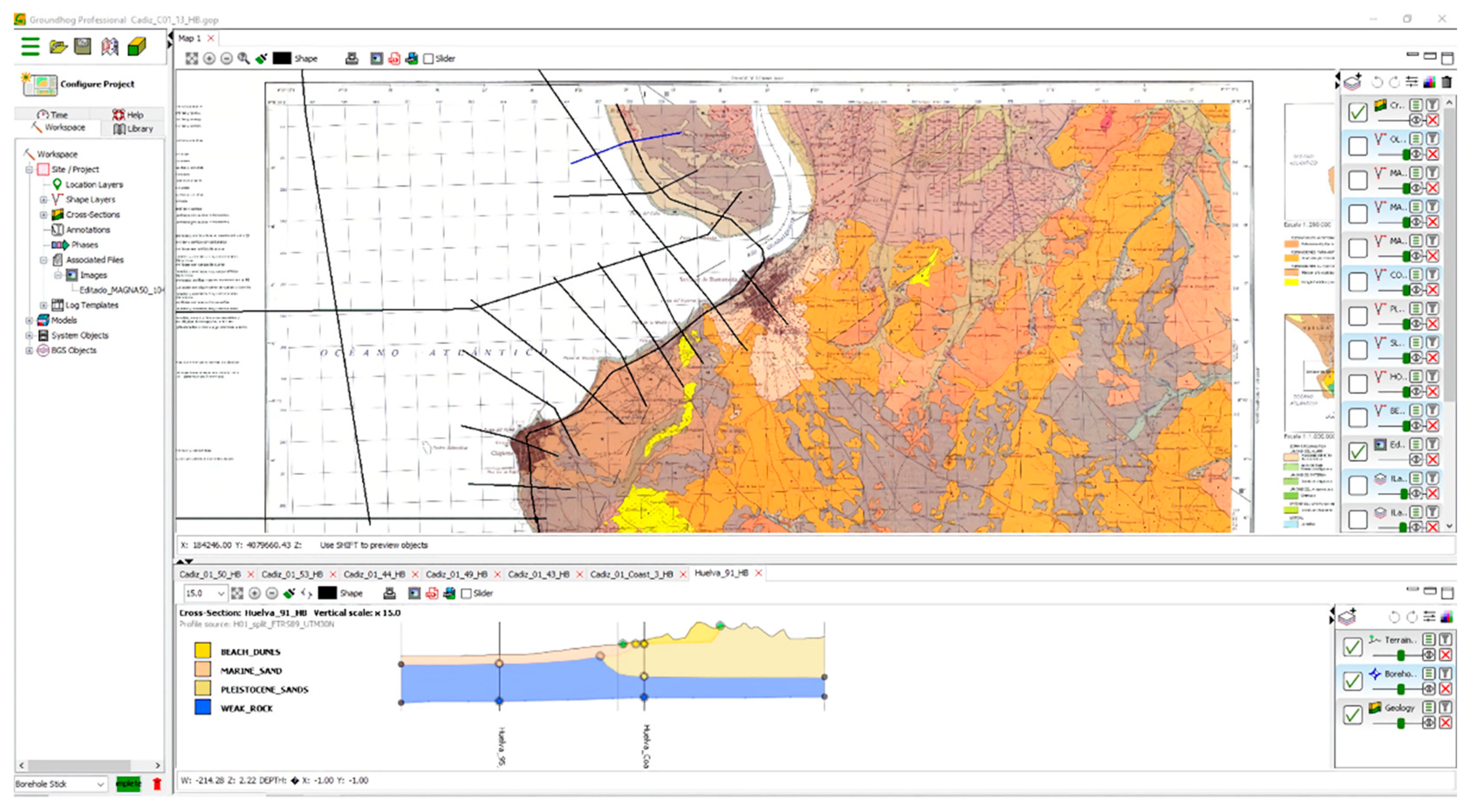
- Geology: 25 Geological maps at a scale 1:50,000 (MAGNA 50) were downloaded from the Spanish Geological and Mining Institute website (IGME, in Spanish for Instituto Geológico y Minero de España) [35]. These maps also include the stratigraphic order, schematic boreholes, and cross-sections.
- Geomorphology: One Seafloor sediment polygon shape layer (SEASED) from the digitalization produced by the Andalusian Government of the Geomorphologic Map of Spain and the Continental Margin at scale 1:1,000,000 compiles by IGME and other institutions and distributed by REDIAM [36] was used as complement information in the definition of the seabed unconsolidated sediments.
3. Methodology
3.1. STMA Elaboration
3.2. Model Querying Tools and Validation
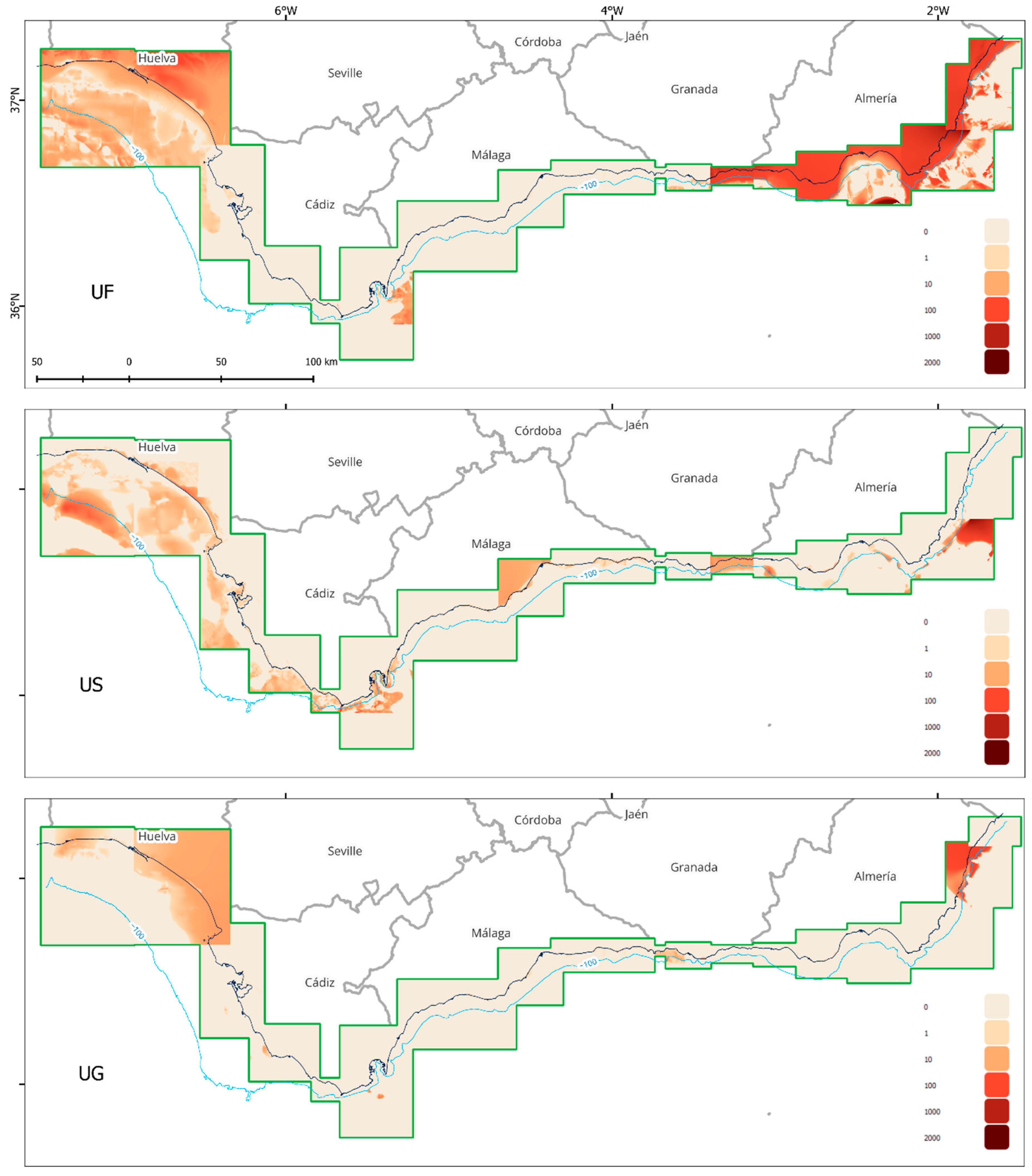
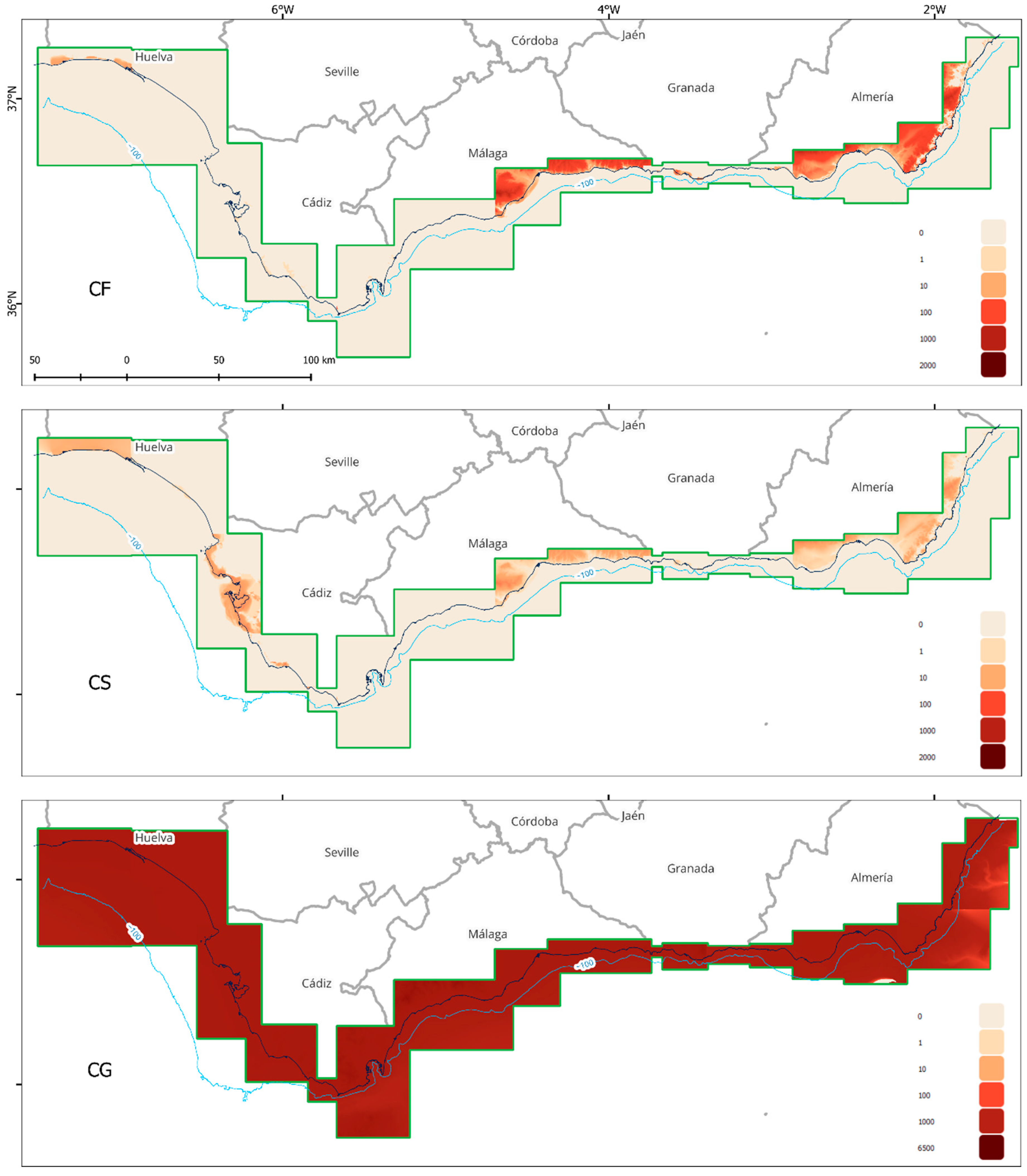
4. Results
4.1. Huelva
4.2. Cádiz
4.3. Málaga
4.4. Granada
4.5. Almería
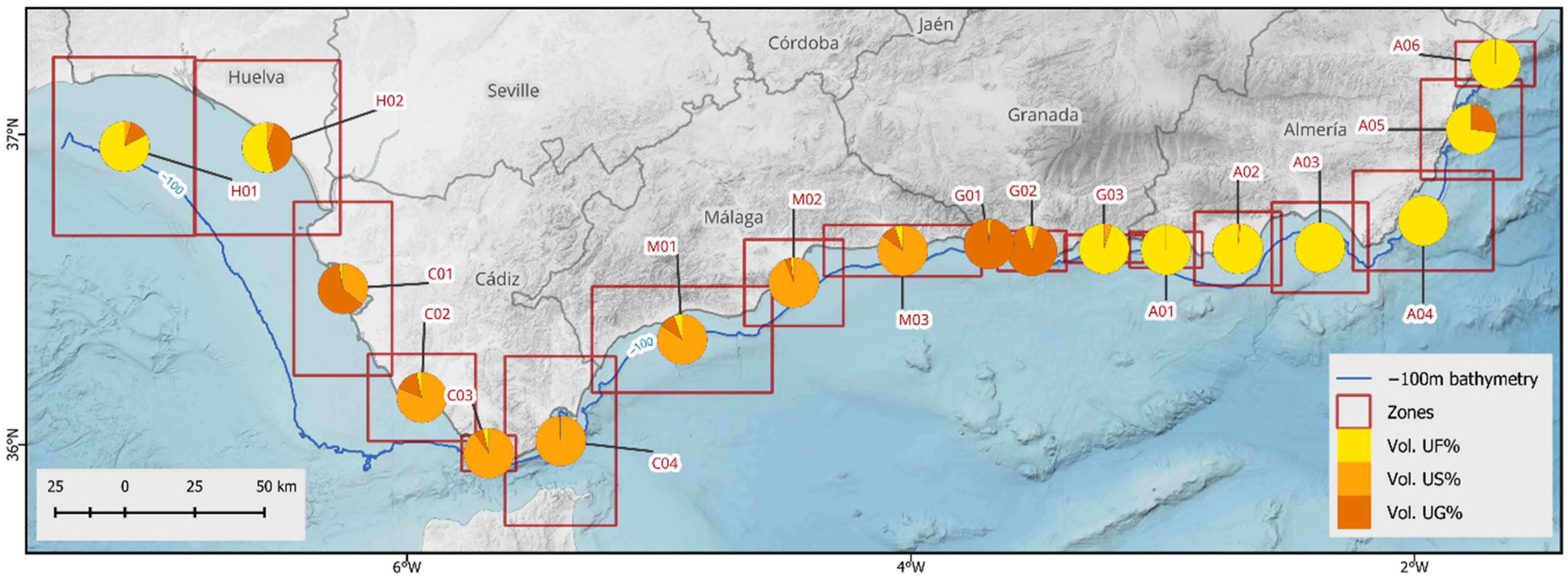
4.6. Model Querying
4.7. Model Validation
5. Discussion and Conclusions
- The baseline depth value chosen of 2050 m has implications in the results of sediment thickness values for the bottom layer, which, for this study, we have assumed is the consolidated gravel layer. The thickness of this layer is assumed to be the elevation difference between the modeled layer and the baseline, resulting in thickness values of the order of 2000 m, which is significantly larger than for the other five layers, whose values are of the order of 1 m to 100s m. This implies that the thickness value for the consolidated gravel layer needs to be interpreted differently than the others (e.g., volume calculations cannot be directly compared with the other five layers). A more accurate representation of the bottom layer will not be solved by using different base depths for the different sections but will require modeling the bedrock surface and resolving the vertical distribution of the different sediment fractions. The implications of the simulation of the coastal landscape evolution using CoastalME are minimal as this software includes, by default, the concept of the active layer via the definition of the availability factor, which assumes that gravel deposits are less available to be transported than sand and fine fractions.
- It is worth discussing the simplified hypothesis considered in the study. In general, the composition of the seabed can be well-described by the sequence of fine, sand, gravel, and unconsolidated and consolidated material, neglecting the above layers if the thickness is zero. However, some regions might be formed by a different sequence of sediment layers.
- The geological maps do not always match the same geological classification, e.g., in Huelva, sheet 998 has alphanumeric codes, e.g., QD for ‘Holocene white sands’ whereas sheet 1047 has numbered unit codes, e.g., 36 ‘Holocene sands, pebbles, and shells’. Also, a map unit code can have a different description on another sheet, e.g., QD is ‘Holocene white sand’ on sheet 998 and ‘Aeolian sand’ on 1033C. Regarding data management, it is worth mentioning the duplication of cross-sections in adjacent model areas and that Groundhog software v2.6 struggled to calculate some of the thickness models, so Huelva had to be split in two for explicit model calculation. In addition to this, it is difficult to keep track of inputting grain size/consolidation information into Groundhog. The model could be improved with more geological information such as boreholes, a shape file of the geology (the geology maps had to be geo-registered and digitized), and a stratigraphic order for the seabed sediments (a shape file showing their distribution was provided, but the stratigraphic order was inferred).
- The spatial scale can also be determinant in some regions. The cell size ranged between 25 and 100 m, which resulted in 5,601,683 cells for the Andalusian coastal zone. Even with that discretization, the spatial scale remains insufficient to model the cliffs that surround the coastline, e.g., in the eastern region of Almeria, where a successive sequence of small rocky coves shapes the coast. On the other hand, the methodology adequately represents the homogeneous sediment pattern of Huelva, Cádiz, and Málaga and the heterogeneity of the sediment of the beaches of Granada (G01 to G03).
- Finally, the queries and the model validation have highlighted the need to include the contribution made by rivers, especially if it is significant, as is the case with the Guadalquivir River. In the area of the large Andalusian rivers, and it likely will also be observed in the Guadiana (H01) and Tinto and Odiel in Huelva (H01 to H02), the contributions that are given make the model differ significantly. Visual observations of the extent of the sediment plume make it evident that it is not being modeled correctly. Furthermore, the area of Almería (A01 to A06) and the east of Granada (G03) must have some geological layer in which attribution may significantly differ. Another notable aspect could be the incidence of contributions along the ramblas, which, during storm episodes, potentially move sediments of mean grain size that reach up to decimeters. That effect is potentially significant in Almería, where more than 30 ramblas split the coastline.
Supplementary Materials
Author Contributions
Funding
Institutional Review Board Statement
Informed Consent Statement
Data Availability Statement
Acknowledgments
Conflicts of Interest
| 1 | |
| 2 |
References
- French, J.R.; Burningham, H. Coastal geomorphology: Trends and challenges. Prog. Phys. Geogr. Earth Environ. 2009, 33, 117–129. [Google Scholar] [CrossRef]
- Burningham, H. Contrasting geomorphic response to structural control: The Loughros estuaries, northwest Ireland. Geomorphology 2008, 97, 300–320. [Google Scholar] [CrossRef]
- Reeve, D.E.; Karunarathna, H.; Pan, S.; Horrillo-Caraballo, J.M.; Różyński, G.; Ranasinghe, R. Data-driven and hybrid coastal morphological prediction methods for mesoscale forecasting. Geomorphology 2016, 256, 49–67. [Google Scholar] [CrossRef]
- Noujas, V.; Thomas, K.V.; Badarees, K.O. Shoreline management plan for a mudbank dominated coast. Ocean. Eng. 2016, 112, 47–65. [Google Scholar] [CrossRef]
- Mingle, J. IPCC Special Report on the Ocean and Cryosphere in a Changing Climate; 0028-7504; New York Review of Books: New York, NY, USA, 2020. [Google Scholar]
- Wolinsky, M.A.; Murray, A.B. A unifying framework for shoreline migration: 2. Application to wave-dominated coasts. J. Geophys. Res. Earth Surf. 2009, 114, F01009. [Google Scholar] [CrossRef]
- Shi, B.; Wang, Y.P.; Wang, L.H.; Li, P.; Gao, J.; Xing, F.; Chen, J.D. Great differences in the critical erosion threshold between surface and subsurface sediments: A field investigation of an intertidal mudflat, Jiangsu, China. Estuar. Coast. Shelf Sci. 2018, 206, 76–86. [Google Scholar] [CrossRef]
- Payo, A.; Williams, C.; Vernon, R.; Hulbert, A.G.; Lee, K.A.; Lee, J.R. Geometrical Analysis of the Inland Topography to Assess the Likely Response of Wave-Dominated Coastline to Sea Level: Application to Great Britain. J. Mar. Sci. Eng. 2020, 8, 866. [Google Scholar] [CrossRef]
- Payo, A.; Favis-Mortlock, D.; Dickson, M.; Hall, J.W.; Hurst, M.D.; Walkden, M.J.A.; Townend, I.; Ives, M.C.; Nicholls, R.J.; Ellis, M.A. Coastal Modelling Environment version 1.0: A framework for integrating landform-specific component models in order to simulate decadal to centennial morphological changes on complex coasts. Geosci. Model Dev. 2017, 10, 2715–2740. [Google Scholar] [CrossRef]
- Payo, A.; French, J.R.; Sutherland, J.; A Ellis, M.; Walkden, M. Communicating Simulation Outputs of Mesoscale Coastal Evolution to Specialist and Non-Specialist Audiences. J. Mar. Sci. Eng. 2020, 8, 235. [Google Scholar] [CrossRef]
- Rattenbury, M.S.; Begg, J.G.; Jones, K.E.; Dabson, O.J.N.; Fitzgerald, R.J.; Payo, A.; Kessler, H.; Wood, B.; Burke, H.; Ellis, M.A.; et al. Application Theme 5—Geohazard and Environmental Risk Applications. In Applied Multidimensional Geological Modeling; John Wiley & Sons: Hoboken, NJ, USA, 2021; pp. 519–554. [Google Scholar]
- Payo, A.; Walkden, M.; Ellis, M.; Barkwith, A.; Favis-Mortlock, D.; Kessler, H.; Wood, B.; Burke, H.; Lee, J. A quantitative assessment of the annual contribution of platform downwearing to beach sediment budget: Happisburgh, England, UK. J. Mar. Sci. Eng. 2018, 6, 113. [Google Scholar] [CrossRef]
- Cobos, M.; Payo, A.; Favis-Mortlock, D.; Burke, H.; Morgan, D.; Jenkins, G.; Smith, H.; Fletcher, T.; Otiñar, P.; Magaña, P.; et al. Importance of Shallow Subsurface and Built Environment Characterization on Assessing Coastal Landscape Morphological Evolution from Hours to Decadal Time Scales: Application to Complex Landforms along Andalucía (Spain) Coastline. In Proceedings of the 39th IAHR World Congress, Granada, Spain, 22 June 2022. [Google Scholar]
- Cobos, M.; Payo, A.; Favis-Mortlock, D.; Burke, H.; Morgan, D.; Jenkins, G.; Smith, H.; Fletcher, T.; Otiñar, P.; Magaña, P.; et al. Modelado de la morfología costera incluyendo elementos antrópicos y sustratos de distintos materiales. Aplicación a sistemas costeros complejos en un tramo del litoral granadino. In Proceedings of the XVI Jornadas Españolas de Ingeniería de Costas y Puertos, Vigo, Spain, 12 May 2022; p. 404. [Google Scholar]
- Molina, R.; Anfuso, G.; Manno, G.; Gracia Prieto, F.J. The Mediterranean Coast of Andalusia (Spain): Medium-Term Evolution and Impacts of Coastal Structures. Sustainability 2019, 11, 3539. [Google Scholar] [CrossRef]
- EEA. WFS Coastal Erosion Trends. 2015. Available online: http://data.adriplan.eu/geoserver/wfs?typename=geonode%3Aerosion_trend&outputFormat=gml2&version=1.0.0&request=GetFeature&service=WFS (accessed on 29 January 2024).
- Manno, G.; Anfuso, G.; Messina, E.; Williams, A.T.; Suffo, M.; Liguori, V. Decadal evolution of coastline armouring along the Mediterranean Andalusia littoral (South of Spain). Ocean Coast. Manag. 2016, 124, 84–99. [Google Scholar] [CrossRef]
- Losada, M.; Baquerizo Azofra, A.; Ortega-Sánchez, M.; Ávila, A. Coastal Evolution, Sea Level, and Assessment of Intrinsic Uncertainty. J. Coast. Res. 2011, 59, 218–228. [Google Scholar] [CrossRef]
- Wilkinson, M.D.; Dumontier, M.; Aalbersberg, I.J.; Appleton, G.; Axton, M.; Baak, A.; Blomberg, N.; Boiten, J.-W.; da Silva Santos, L.B.; Bourne, P.E.; et al. The FAIR Guiding Principles for scientific data management and stewardship. Sci. Data 2016, 3, 160018. [Google Scholar] [CrossRef]
- Kessler, H.; Mathers, S.; Sobisch, H.-G. The capture and dissemination of integrated 3D geospatial knowledge at the British Geological Survey using GSI3D software and methodology. Comput. Geosci. 2009, 35, 1311–1321. [Google Scholar] [CrossRef]
- BGS. BGS Groundhog v2.8. Available online: https://www.bgs.ac.uk/technologies/software/groundhog/ (accessed on 29 January 2024).
- INE. Demografía y Población. Available online: https://www.ine.es/dynInfo/Infografia/Territoriales/capituloGraficos.html#!mapa (accessed on 15 November 2023).
- IECA. Directorio de Empresas y Establecimientos con Actividad Económica en Andalucía. 2021. Available online: https://www.juntadeandalucia.es/institutodeestadisticaycartografia/direst/index.htm (accessed on 29 January 2024).
- IECA. Spatial Distribution of Andalusia Population. 2021. Available online: https://www.juntadeandalucia.es/institutodeestadisticaycartografia/distribucionpob/index.htm (accessed on 29 January 2024).
- IECA. Encuesta de Coyuntura Turística de Andalucía 2022. Available online: https://www.juntadeandalucia.es/institutodeestadisticaycartografia/turismo/index.htm (accessed on 29 January 2024).
- Morales, J.A. (Ed.) The Spanish Coastal Systems. Dynamic Processes, Sediments and Management, 1st ed.; Springer: Berlin/Heidelberg, Germany, 2019; p. 823. [Google Scholar]
- Liquete, C.; Arnau, P.; Canals, M.; Colas, S. Mediterranean river systems of Andalusia, southern Spain, and associated deltas: A source to sink approach. Mar. Geol. 2005, 222–223, 471–495. [Google Scholar] [CrossRef]
- Jodar, J.M.; Voulgaris, G.; Luna del Barco, A.; Gutierrez-mas, J.M. Wave and Current Conditions and Implications for the Distribution of sediment in the Bay of Cadiz (Andalusia, SW Spain). In Proceedings of the Litoral 2002, Porto, Portugal, 22–26 September 2002. [Google Scholar]
- Hearn, G.J. Geology, geomorphology and geohazards on a section of the Betic coastline, southern Spain. Q. J. Eng. Geol. Hydrogeol. 2019, 52, 208–219. [Google Scholar] [CrossRef]
- IGN. Digital Terrain Model with 25-metre grid pitch (DTM25) of Spain. MDT25. 2015. Available online: https://www.idee.es/csw-inspire-idee/srv/spa/catalog.search?#/metadata/spaignMDT25 (accessed on 29 January 2024).
- Guisado, E.; Malvárez, G.C. Multiple Scale Morphodynamic mapping: Methodological Considerations and Applications for the Coastal Atlas of Andalusia. J. Coast. Res. 2009, 56, 1513–1517. [Google Scholar]
- MMAA. Ecocartography of Cádiz, Málaga, Granada and Almería. Ecocartography. 2012. Available online: https://portalrediam.cica.es/descargas/index.php/s/mxHMWXyHfrCxyNK?path=%2F08_AMBITOS_INTERES_AMBIENTAL%2F02_LITORAL_MARINO%2F06_BATIMETRIAS (accessed on 29 January 2024).
- EMODnet. DTM 2020. 2020. Available online: https://emodnet.ec.europa.eu/en (accessed on 29 January 2024).
- CMAOT. Coastline 2013. 2013. Available online: https://portalrediam.cica.es/descargas/index.php/s/mxHMWXyHfrCxyNK?path=%2F08_AMBITOS_INTERES_AMBIENTAL%2F02_LITORAL_MARINO%2F02_GEOLOGIA%2FLinea_Costa_2013 (accessed on 29 January 2024).
- IGME. Mapa Geológico de España a escala 1:50.000 (2ª Serie). MAGNA50. Available online: http://info.igme.es/cartografiadigital/geologica/Magna50.aspx (accessed on 29 January 2024).
- IGME; IEO; Spanish-Universities. Geomorphologic Map of Spain and the Continental Margin at scale 1:1,000,000. 1979. Available online: https://portalrediam.cica.es/descargas/index.php/s/mxHMWXyHfrCxyNK?path=%2F08_AMBITOS_INTERES_AMBIENTAL%2F02_LITORAL_MARINO%2F02_GEOLOGIA%2FGeomorfologico_marino (accessed on 29 January 2024).
- Barber, C.B.; Dobkin, D.P.; Huhdanpaa, H. The quickhull algorithm for convex hulls. ACM Trans. Math. Softw. 1996, 22, 469–483. [Google Scholar] [CrossRef]
- QGIS.org. QGIS Geographic Information System. Open Source Geospatial Foundation. Available online: https://qgis.org/ (accessed on 29 January 2024).
- Serrano, M.A.; Díez-Minguito, M.; Ortega-Sánchez, M.; Losada, M.A. Continental shelf waves on the Alborán sea. Cont. Shelf Res. 2015, 111, 1–8. [Google Scholar] [CrossRef]
- Fernández-Salas, L.M.; Durán, R.; Lobo, F.J.; Ribó, M.; Canals, M. Shelves of the Iberian Peninsula and the Balearic Islands (I): Morphology and sediment types. Bol. Geol. Y Min. 2015, 126, 327–376. [Google Scholar]
- Gracia, F.-J.; Morales, J.-A.; Castañeda, C.; Plomaritis, T.A. Shallow lacustrine versus open ocean coastal clastic deposits: Morphosedimentary diagnostic indicators and interpretation. Sediment. Geol. 2021, 423, 105981. [Google Scholar] [CrossRef]
- Jabaloy-Sánchez, A.; Lobo, F.J.; Azor, A.; Martín-Rosales, W.; Pérez-Peña, J.V.; Bárcenas, P.; Macías, J.; Fernández-Salas, L.M.; Vázquez-Vílchez, M. Six thousand years of coastline evolution in the Guadalfeo deltaic system (southern Iberian Peninsula). Geomorphology 2014, 206, 374–391. [Google Scholar] [CrossRef]
- López, P.M.; Payo, A.; Ellis, M.A.; Criado-Aldeanueva, F.; Jenkins, G.O. A Method to Extract Measurable Indicators of Coastal Cliff Erosion from Topographical Cliff and Beach Profiles: Application to North Norfolk and Suffolk, East England, UK. J. Mar. Sci. Eng. 2020, 8, 20. [Google Scholar] [CrossRef]
- Walkden, M.; Dickson, M. Equilibrium erosion of soft rock shores with a shallow or absent beach under increased sea level rise. Mar. Geol. 2008, 251, 75–84. [Google Scholar] [CrossRef]


| Color | Modeled Unit | Lithology | % Fine | % Sand | % Gravel | Consolidated/ Unconsolidated |
|---|---|---|---|---|---|---|
 | Beach and dunes | Holocene beach deposits and sand dunes | 5 | 85 | 10 | Unconsolidated |
 | Holocene silts and clays | Holocene estuarine silts and clays | 95 | 5 | 0 | Consolidated |
 | Slope deposits | Loose sand and gravel on steep slopes | 33 | 33 | 34 | Unconsolidated |
 | Older silts and clays | Silts and clays at higher elevations and further inland | 95 | 5 | 0 | Consolidated |
 | Marine clay | Offshore seafloor clay 1 | 100 | 0 | 0 | Unconsolidated |
 | Marine sand | Offshore sand deposits 1 | 0 | 100 | 0 | Unconsolidated |
 | Marine gravel | Offshore gravel deposits 1 | 0 | 0 | 100 | Unconsolidated |
 | Pleistocene sands | Older sand deposits | 0 | 95 | 5 | Consolidated |
 | Conglomerate | Cemented sand, gravel, and cobbles | 0 | 90 | 10 | Consolidated |
 | Weak rock | Limestone/mudstone | 0 | 0 | 100 | Consolidated |
 | Strong rock | Volcanic and crystalline basement rocks | 0 | 0 | 100 | Consolidated |
| Zone | Cell Size (m) | Num. of Cells | Unconsolidated | Consolidated | |||||||
|---|---|---|---|---|---|---|---|---|---|---|---|
| Grain | Mean (m) | Median (m) | Min (m) | Max (m) | Mean (m) | Median (m) | Min (m) | Max (m) | |||
| A01 | 50 | 522 × 258 | F | 149.5 | 117.1 | 0.0 | 877.9 | 1943.0 | 1992.8 | 0.0 | 2096.2 |
| S | 3.3 | 0.0 | 0.0 | 106.7 | 0.0 | 0.0 | 0.0 | 1.1 | |||
| G | 0.0 | 0.0 | 0.0 | 7.7 | 1864.3 | 1903.5 | 1533.8 | 1912.8 | |||
| A02 | 50 | 623 × 527 | F | 134.3 | 163.7 | 0.0 | 370.2 | 67.6 | 0.0 | 0.0 | 1095.3 |
| S | 0.2 | 0.0 | 0.0 | 23.8 | 3.6 | 0.0 | 0.0 | 57.6 | |||
| G | 0.0 | 0.0 | 0.0 | 2.8 | 1864.6 | 1870.0 | 0.0 | 2064.5 | |||
| A03 | 50 | 692 × 648 | F | 86.2 | 16.1 | 0.0 | 1804.8 | 17.2 | 0.0 | 0.0 | 799.9 |
| S | 0.7 | 0.0 | 0.0 | 55.0 | 0.9 | 0.0 | 0.0 | 42.1 | |||
| G | 0.0 | 0.0 | 0.0 | 1.8 | 1772.4 | 1877.3 | 0.0 | 1993.7 | |||
| A04 | 100 | 504 × 358 | F | 238.7 | 100.2 | 0.0 | 1960.4 | 28.3 | 0.0 | 0.0 | 614.8 |
| S | 84.8 | 0.0 | 0.0 | 1621.4 | 1.5 | 0.0 | 0.0 | 32.4 | |||
| G | 0.0 | 0.0 | 0.0 | 2.9 | 1275.5 | 1410.2 | 0.0 | 1873.3 | |||
| A05 | 50 | 726 × 716 | F | 104.2 | 13.8 | 0.0 | 410.1 | 29.3 | 0.0 | 0.0 | 840.8 |
| S | 0.0 | 0.0 | 0.0 | 39.8 | 1.5 | 0.0 | 0.0 | 44.3 | |||
| G | 47.6 | 0.0 | 0.0 | 322.6 | 1284.7 | 1453.8 | 0.0 | 1787.7 | |||
| A06 | 50 | 570 × 320 | F | 173.0 | 179.0 | 0.0 | 720.8 | 0.3 | 0.0 | 0.0 | 383.2 |
| S | 0.0 | 0.0 | 0.0 | 15.6 | 0.4 | 0.0 | 0.0 | 1601.2 | |||
| G | 0.0 | 0.0 | 0.0 | 1.8 | 1601.0 | 1788.7 | 0.0 | 1975.9 | |||
| C01 | 75 | 472 × 831 | F | 0.3 | 0.0 | 0.0 | 10.9 | 0.0 | 0.0 | 0.0 | 9.5 |
| S | 1.3 | 0.0 | 0.0 | 44.1 | 3.5 | 0.0 | 0.0 | 2499.7 | |||
| G | 0.0 | 0.0 | 0.0 | 5.6 | 2040.3 | 2035.4 | 1962.1 | 2182.6 | |||
| C02 | 50 | 780 × 630 | F | 0.0 | 0.0 | 0.0 | 12.4 | 0.0 | 0.0 | 0.0 | 5.9 |
| S | 1.3 | 0.0 | 0.0 | 240.9 | 0.2 | 0.0 | 0.0 | 55.4 | |||
| G | 0.1 | 0.0 | 0.0 | 18.3 | 2059.8 | 2055.2 | 1943.2 | 2481.7 | |||
| C03 | 25 | 780 × 508 | F | 0.1 | 0.0 | 0.0 | 35.1 | 0.0 | 0.0 | 0.0 | 0.0 |
| S | 4.3 | 0.0 | 0.0 | 97.6 | 0.0 | 0.0 | 0.0 | 28.7 | |||
| G | 0.0 | 0.0 | 0.0 | 6.9 | 1995.6 | 2017.3 | 0.0 | 2524.5 | |||
| C04 | 100 | 399 × 607 | F | 2.0 | 0.0 | 0.0 | 112.9 | 0.1 | 0.0 | 0.0 | 304.4 |
| S | 2.4 | 0.0 | 0.0 | 412.7 | 0.0 | 0.0 | 0.0 | 16.0 | |||
| G | 0.1 | 0.0 | 0.0 | 84.2 | 1893.2 | 2024.5 | 1073.9 | 2866.7 | |||
| G01 | 25 | 592 × 240 | F | 0.0 | 0.0 | 0.0 | 0.3 | 0.2 | 0.0 | 0.0 | 22.0 |
| S | 0.0 | 0.0 | 0.0 | 0.7 | 0.0 | 0.0 | 0.0 | 1.2 | |||
| G | 4.4 | 1.0 | 0.0 | 2040.4 | 2068.4 | 2021.3 | 0.0 | 6403.3 | |||
| G02 | 25 | 996 × 575 | F | 0.9 | 0.0 | 0.0 | 71.7 | 2.0 | 0.0 | 0.0 | 91.6 |
| S | 0.0 | 0.0 | 0.0 | 1.6 | 0.1 | 0.0 | 0.0 | 11.6 | |||
| G | 1.8 | 0.0 | 0.0 | 2049.2 | 2034.6 | 1997.0 | 0.0 | 2956.0 | |||
| G03 | 25 | 1140 × 399 | F | 296.4 | 300.8 | 0.0 | 867.7 | 0.0 | 0.0 | 0.0 | 1.9 |
| S | 15.9 | 16.3 | 0.0 | 45.7 | 0.0 | 0.0 | 0.0 | 387.8 | |||
| G | 0.0 | 0.0 | 0.0 | 1.9 | 1650.5 | 1653.2 | 0.0 | 1724.3 | |||
| H01 | 100 | 510 × 640 | F | 10.4 | 7.1 | 0.0 | 99.0 | 0.3 | 0.0 | 0.0 | 25.8 |
| S | 6.9 | 0.0 | 0.0 | 95.3 | 1.0 | 0.0 | 0.0 | 13.1 | |||
| G | 0.5 | 0.0 | 0.0 | 24.8 | 1875.8 | 1959.7 | 1474.9 | 2031.1 | |||
| H02 | 100 | 525 × 625 | F | 24.7 | 10.7 | 0.0 | 135.4 | 0.0 | 0.0 | 0.0 | 23.4 |
| S | 2.5 | 0.0 | 0.0 | 91.3 | 0.0 | 0.0 | 0.0 | 28.1 | |||
| G | 8.8 | 9.2 | 0.0 | 28.8 | 2013.5 | 2019.9 | 1878.6 | 2048.8 | |||
| M01 | 100 | 648 × 381 | F | 0.0 | 0.0 | 0.0 | 9.0 | 0.0 | 0.0 | 0.0 | 6.4 |
| S | 0.0 | 0.0 | 0.0 | 27.8 | 0.0 | 0.0 | 0.0 | 4.7 | |||
| G | 0.0 | 0.0 | 0.0 | 9.2 | 1935.9 | 1972.1 | 1099.7 | 3478.8 | |||
| M02 | 100 | 356 × 310 | F | 0.0 | 0.0 | 0.0 | 2.0 | 58.8 | 0.0 | 0.0 | 1067.2 |
| S | 5.4 | 0.0 | 0.0 | 132.6 | 7.3 | 0.0 | 0.0 | 2509.0 | |||
| G | 0.0 | 0.0 | 0.0 | 3.9 | 1945.4 | 1997.5 | 0.0 | 2146.2 | |||
| M03 | 100 | 566 × 184 | F | 0.0 | 0.0 | 0.0 | 6.8 | 68.0 | 0.0 | 0.0 | 966.8 |
| S | 0.3 | 0.0 | 0.0 | 116.0 | 3.6 | 0.0 | 0.0 | 50.9 | |||
| G | 0.0 | 0.0 | 0.0 | 13.6 | 1943.0 | 1992.8 | 0.0 | 2096.2 | |||
| Map | Unit Code | Description | Modeled Unit | |
|---|---|---|---|---|
| 998 | QD | Holocene white sands | Beach and dunes | |
| 998 | QE | Holocene white sands | Beach and dunes | |
| 998 | QG | Quaternary conglomerates and red clays | Beach and dunes | |
| 998 | QM | Holocene silts, clays, and sands | Holocene silts and clays | |
| 998 | QAI | Holocene sands and silts | Holocene silts and clays | |
| 998 | TB/ CG-Q/2 | Pliocene red clayey sands and gravels | Pleistocene sands | |
| 998 | TB/21 | Pliocene sandy silts and grey-yellow sands | Pleistocene sands | |
| 999 | QP | Quaternary sand | Beach and dunes | |
| 999 | QD2 | Quaternary sand | Beach and dunes | |
| 999 | Qt | Quaternary peat | Beach and dunes | |
| 999 | QAI | Quaternary silts and sands | Holocene silts and clays | |
| 999 | TB-2Q | Base Quaternary sands | Pleistocene sands | |
| 999 | QT2 | Quaternary gravels, sands, silts, clays | Slope deposits | |
| 1033 | QP2 | Quaternary sand | Beach and dunes | |
| 1033 | QP1 | Quaternary sand | Beach and dunes | |
| 1033 | QAI | Quaternary silts and sands | Beach and dunes | |
| 1033 | QD2 | Quaternary sand | Beach and dunes | |
| 1033 | QD | Quaternary sand | Beach and dunes | |
| 1033 | TB-Q2 | Pliocene sand | Pleistocene sands | |
| 1047 | 36 | Holocene sands, pebbles, and shells | Beach and dunes | |
| 1047 | 32 | Holocene sands | Beach and dunes | |
| 1047 | 31 | Holocene sands, pebbles/cobbles and shells | Beach and dunes | |
| 1047 | 30 | Holocene sand, poss dunes | Beach and dunes | |
| 1047 | 23 | Holocene sands, pebbles/cobbles and shells | Beach and dunes | |
| 1047 | 10 | Pleistocene/Quaternary quartz sands with some quartz and quartzite cobbles | Conglomerate | |
| 1047 | 12 | Pleistocene conglomerate with carbonate-rich sandstone | Conglomerate | |
| 1047 | 7 | - | Conglomerate | |
| 1047 | 19 | Holocene greenish marls with hydromorphic soils (developed in waterlogged conditions) | Older silts and clays | |
| 1047 | 18 | Pleistocene sand | Pleistocene sands | |
| 1047 | 16 | Pleistocene sands and clays with carbonate cobbles | Pleistocene sands | |
| 1047 | 15 | Pleistocene clayey sands with quartz cobbles | Pleistocene sands | |
| 1047 | 13 | Pleistocene clayey sands with quartz cobbles | Pleistocene sands | |
| 1047 | 3 | Tertiary siliceous white marls with radiolaria and diatoms (weak bedrock) | Weak rock | |
| 1033C | QP | Beach deposits | Beach and dunes | |
| 1033C | QT | Peat | Beach and dunes | |
| 1033C | QD2 | Barrier dunes | Beach and dunes | |
| 1033C | QD1 | Ancient dunes | Beach and dunes | |
| 1033C | QD | Aeolian sand | Beach and dunes | |
| 1033C | TB-Q2 | Pliocene sand | Pleistocene sands | |
| STMA Zone | Median Elev. from Reference (m) | Mean Elev. from Reference (m) | %US | %UG | %UF |
|---|---|---|---|---|---|
| A01 | 2048 | 2048 | 0.17 | 0.02 | 99.80 |
| A02 | 2051 | 2053 | 1.36 | 0.16 | 98.47 |
| A03 | 2049 | 2052 | 0.18 | 0.01 | 99.79 |
| A04 | 2060 | 2067 | 0.01 | 0.00 | 99.98 |
| A05 | 2053 | 2060 | 0.039 | 27.316 | 72.645 |
| A06 | 2055 | 2058 | 0.00 | 0.00 | 99.99 |
| C01 | 2051 | 2051 | 35.66 | 61.93 | 2.40 |
| C02 | 2049 | 2049 | 80.98 | 15.67 | 3.34 |
| C03 | 2049 | 2050 | 89.86 | 6.15 | 3.98 |
| C04 | 2054 | 2057 | 99.12 | 0.58 | 0.29 |
| G01 | 2050 | 2054 | 1.73 | 97.39 | 0.86 |
| G02 | 2049 | 2052 | 4.80 | 90.15 | 5.03 |
| G03 | 2049 | 2052 | 5.09 | 0.00 | 94.90 |
| H01 | 2051 | 2050 | 4.61 | 12.59 | 82.79 |
| H02 | 2051 | 2051 | 4.83 | 40.94 | 54.22 |
| M01 | 2052 | 2052 | 84.23 | 10.35 | 5.41 |
| M02 | 2052 | 2053 | 94.00 | 3.99 | 1.99 |
| M03 | 2050 | 2054 | 84.98 | 10.02 | 4.99 |
Disclaimer/Publisher’s Note: The statements, opinions and data contained in all publications are solely those of the individual author(s) and contributor(s) and not of MDPI and/or the editor(s). MDPI and/or the editor(s) disclaim responsibility for any injury to people or property resulting from any ideas, methods, instructions or products referred to in the content. |
© 2024 by the authors. Licensee MDPI, Basel, Switzerland. This article is an open access article distributed under the terms and conditions of the Creative Commons Attribution (CC BY) license (https://creativecommons.org/licenses/by/4.0/).
Share and Cite
Torrecillas, C.; Payo, A.; Cobos, M.; Burke, H.; Morgan, D.; Smith, H.; Jenkins, G.O. Sediment Thickness Model of Andalusia’s Nearshore and Coastal Inland Topography. J. Mar. Sci. Eng. 2024, 12, 269. https://doi.org/10.3390/jmse12020269
Torrecillas C, Payo A, Cobos M, Burke H, Morgan D, Smith H, Jenkins GO. Sediment Thickness Model of Andalusia’s Nearshore and Coastal Inland Topography. Journal of Marine Science and Engineering. 2024; 12(2):269. https://doi.org/10.3390/jmse12020269
Chicago/Turabian StyleTorrecillas, Cristina, Andres Payo, Manuel Cobos, Helen Burke, Dave Morgan, Helen Smith, and Gareth Owen Jenkins. 2024. "Sediment Thickness Model of Andalusia’s Nearshore and Coastal Inland Topography" Journal of Marine Science and Engineering 12, no. 2: 269. https://doi.org/10.3390/jmse12020269