Characterizing the Variability of a Physical Driver of North Atlantic Right Whale Foraging Habitat Using Altimetric Indices

Abstract

Physical ocean circulation features, especially the Gaspé Current (GC) intrusion, influence the transport and aggregation of whale prey, thereby influencing the whale foraging habitat in the Gulf of St. Lawrence (GSL), Canada. We employ satellite altimetry-derived sea level anomaly (SLA) indices to monitor interannual variations in the intensity of the GC in the North Atlantic Right Whale (Eubalaena glacialis; NARW) habitat in the GSL. Measurements of surface slope and volume transport are taken from the SLA profiles along a repeating ground track of the Jason-2/3 satellites. These are employed as complementary proxies in characterizations of physical processes in the GSL. The relationship between altimetric indices and indices of zooplankton abundance are explored in the southern GSL. Results demonstrate that an altimetric index estimated from surface slope (Index${}_{slope-half}$) is correlated with river discharge of the St. Lawrence River and can be utilized to infer variations in GC intensities. Time series of the altimetric indices during 2009–2021 are found to exhibit interannual and seasonal environmental variability, which influence transport into the southern GSL. As captured by the altimetric indices, these features of the surface ocean circulation can be linked to zooplankton variations in the Shediac Valley, where NARWs are frequently observed. Therefore, in linking physical drivers of ocean dynamics to the NARW foraging habitat, variations in these indices can also potentially help describe some features of the distribution patterns of NARW sightings in this area.

1. Introduction

The ocean circulation is a fundamental ecosystem driver that affects water masses, nutrient supplies, growth of phytoplankton, structure of pelagic food webs, and thus, the suitability of the whale foraging habitat [1,2,3,4]. Oceanographic conditions largely determine the spatiotemporal distributions of prey fields [2]. Previously, high densities of zooplankton have been observed and modelled in near-surface convergence zones associated with fronts [5,6,7], internal waves [8,9,10], and Langmuir circulation [11]. Sub-mesoscale and mesoscale oceanic features (such as coastal currents, eddies and their associated gradients or fronts) are able to aggregate whale prey [12]. Prey patches are formed through small-scale biophysical interactions in which zooplankton movements interact with sub-mesoscale ocean convergence or divergence features [13]. Whales appear to be capable of detecting patches of high concentrations of prey; they tend to remain within these prey patches when feeding (e.g., Mayo and Marx [14]). Whale foraging habitats have been primarily characterized by high densities of their prey species and the physical conditions that facilitate the aggregation of dense zooplankton patches of these prey [14,15,16]. Thus, characterizing ocean circulation features is crucial in studying whale foraging habitats.

The global satellite altimeter data record now covers multiple decades, and is used to study the long-term ocean dynamics, surface current variability and sea level [17,18]. Satellite altimeter data applications in association with biological productivity of marine ecosystems have been explored in previous studies. For example, altimetry observations were used to reveal North Atlantic current variability over the last two decades, and shape the spatial distributions of coccolithophore [19]; altimetry-derived surface currents were used to investigate the interactions of the seasonal distribution of Mediterranean fin whales with the ocean circulation at different spatiotemporal scales [20]. These studies suggest that oceanic features create favorable foraging grounds for whales searching for aggregated prey. However, applications of altimetry data to investigate the connections between physical drivers and zooplankton prey related to the presence of the North Atlantic Right Whale (Eubalaena glacialis; NARW) in the Gulf of St. Lawrence (GSL) have not been made.

In this introduction section, we begin by describing the prominent GSL circulation features and the recent NARW sightings. We then discuss the use of altimetry to study sea surface current variability and sea level characteristics, and we suggest that variability in the related indices for altimetry features can be useful in estimating variations in NARW prey habitats. An outline of the remainder of the paper is given at the end of Section 1.3.

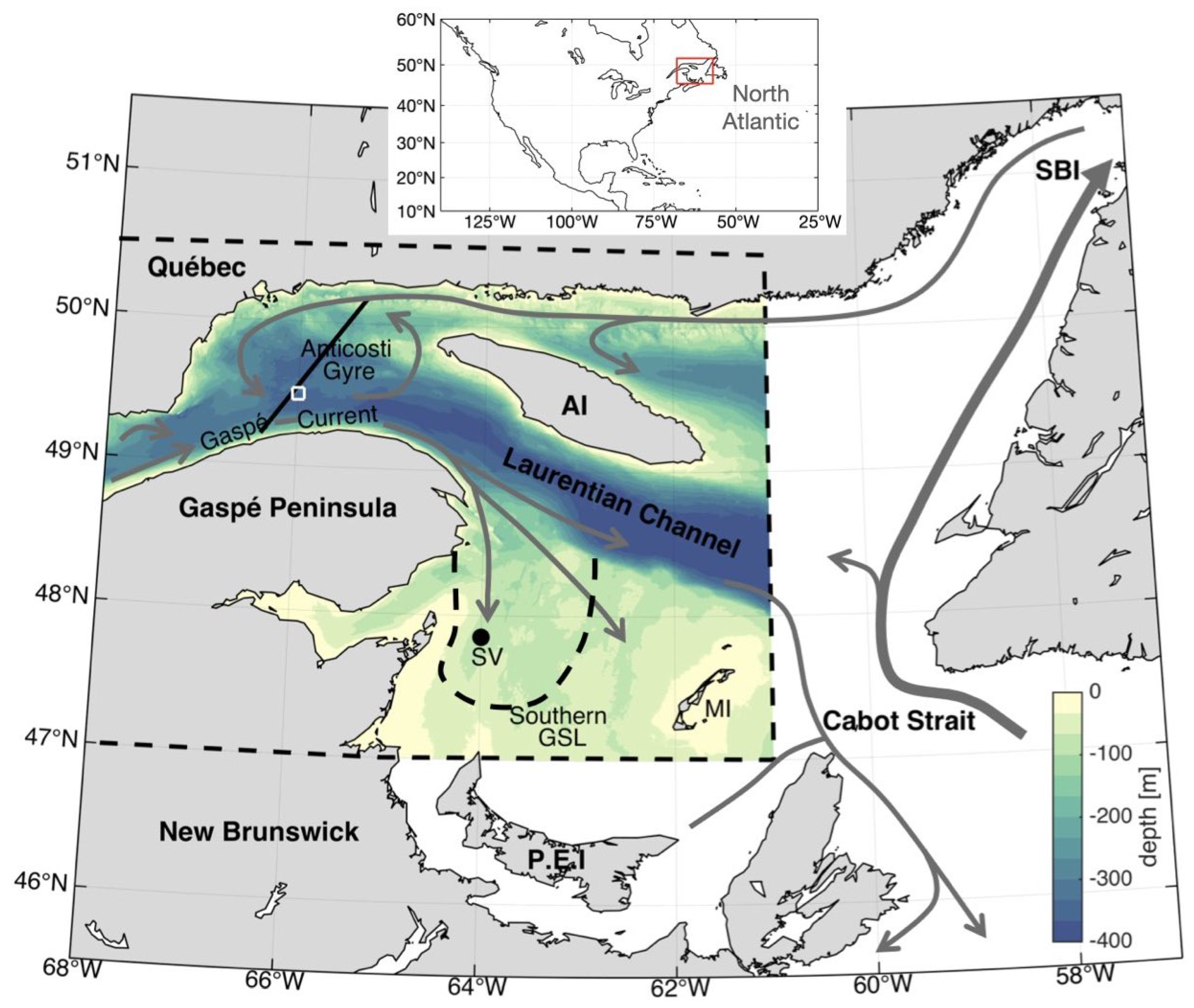
1.1. GSL Circulation

The GSL is a semi-enclosed sea that communicates with the Atlantic Ocean through the Cabot Strait and the Strait of Belle Isle (Figure 1). A major topographic feature of the GSL is the Laurentian Channel, a continuous trough over 300 m deep that runs 1100 km from the edge of the continental shelf to the St. Lawrence Estuary. The southern GSL is a wide plateau with depths that rarely exceed 80 m [21,22]. Large amounts of freshwater enter the western GSL from the St. Lawrence River. A smaller transport of water occurs via the northeastern entrance (Strait of Belle Isle). Buoyancy forcing of the GSL circulation by the freshwater input and surface heat flux exhibit strong seasonal variability [21,23]. Runoff starts to increase in March, reaching a maximum in May at about 20,000 m${}^3$/s, and decreases from June to September to a value of about 13,000 m${}^3$/s. Typically, heat flux from the atmosphere peaks in June, and wind-stress forcing (an important source of kinetic energy) peaks in fall and winter, prior to the onset of winter ice cover. Wind directions are highly variable throughout the year, but are predominantly from the southwest in summer, west in fall, and northwest in winter [24]. Other factors are also known to impact the GSL system, such as tidal forcing and other oceanic forcing from the North Atlantic [21].

Notable features of near surface circulation in the northwest GSL (nwGSL, Figure 1) are the Gaspé Current (GC) and Anticosti Gyre. The GC is a strong baroclinic coastal jet along the north shore of Gaspé Peninsula, which is driven by the runoff from the St. Lawrence Estuary into the GSL [21,25,26]. It is strong and warm in the summer and cold and weak in the winter [23]. The Anticosti Gyre is a cyclonic circulation in the nwGSL becoming more evident during summer. This is the portion of the GC that recirculates cyclonically within the nwGSL and combines with a barotropic westward jet (an extension of the Labrador Shelf Current) along the north shore of the GSL [21,26].

The main branch of the GC continues eastward along the Gaspé Peninsula, carrying buoyant estuarine waters into the southern GSL (sGSL) [23,26]. The maintenance and strength of the GC and Anticosti Gyre are determined in part by the freshwater outflow from the estuary and westward flow along the north shore of the GSL [23,26,27]. In turn, the St. Lawrence River is the main source of freshwater discharge into the estuary and the GSL. The freshwater from the St. Lawrence River exerts a fundamental control on stratification and dynamical forcing on the GC [21]. Numerical simulations confirm the dominant role of river runoff on the flow pattern of the GC (e.g., Sheng [26]). A seasonal increase in the St. Lawrence River discharge (maximum flux difference is ∼9000 m${}^3$/s) typically results in a strengthening of the GC by up to 0.1 m/s [28].

1.2. NARW in the sGSL

In recent years, the GSL has become recognized as a NARW aggregation area and feeding ground from spring to fall [13,29,30]. Sightings of NARWs have been frequent in the sGSL, especially in the vicinity of the Shediac Valley, but also to the north and west of Anticosti Island [31,32]. During systematic surveys in the sGSL in 2017–2019, the first visual observations of NARW have occurred around mid-May and the latest NARW observations were around mid-November. Passive acoustic monitoring from 2010 to 2018 has revealed NARWs in the sGSL from late April through mid-January [33]. During this time, the frequency of detections has increased substantially in May, with the peak acoustic detections occurring between August and the end of October [31,34].

Spatial and temporal variations in whale prey biomass in the GSL have been examined by Lehoux et al. [29], Gavrilchuk et al. [35], and Blais et al. [36]. Sorochan et al. [13] reviewed the components of NARW diet, mainly copepods of the genus Calanus. Calanus finmarchicus is widely distributed in the western North Atlantic and is a major component of the NARW diet [13,16,37,38]. Calanus hyperboreus and Calanus glacialis are two arctic species of Calanus that are important prey [13,29]. The larger Calanus hyperboreus dominates prey biomass in the sGSL during spring and summer [29]. Pseudocalanus spp. are numerically abundant copepods that are also potential NARW prey [29]. Plourde et al. [39] represented the spatial climatology of water column integrated biomass of Calanus spp. in the spring and in summer-fall in the GSL. High Calanus spp. was observed in the northern GSL and in the southwestern GSL. Horizontal distributions of Calanus finmarchicus and Pseudocalanus spp. were widespread, whereas those of Calanus hyperboreus and Calanus glacialis were centred in the interior of the sGSL [40]. Brennan et al. [38] investigated the effect of mechanistic drivers in Calanus abundance in the NARW foraging habitat. Calanus variability is strongly influenced by ocean circulation, such as advection from upstream, which is linked to river runoff and winds on the coastal GC in late spring and summer. Previous studies found that the GC is the main pathway for zooplankton transport and aggregation in the sGSL, likely influencing whale distribution and behavior patterns [3,38,41,42,43]. Plourde and Runge [43] proposed that the circulation in the lower St. Lawrence Estuary acts as a ‘Calanus pump’, with imports of diapausing Calanus finmarchicus copepodites by deep inflow and exports of early active stages by surface outflow. The GC is a freshwater pathway to the southern GSL, providing Calanus spp. from the St. Lawrence Estuary and nwGSL [3,38,41]. As a physical driver of zooplankton supply to the sGSL, the strength of the GC can be considered a potential predictor of NARW foraging habitat variations.

1.3. Satellite Altimetry to Monitor Physical Drivers of Prey Supply

To understand ocean dynamics in the GSL, in situ measurements and numerical models have been used widely [21,23,25,26]. However, it is difficult to continuously monitor the mesoscale features and GC pathway using in situ measurements from traditional ship and aircraft surveys. Satellite altimetry has been applied to study sea level and surface current variability under all weather conditions, with high resolution and short revisit times (e.g., Abdalla et al. [17], Han [22], Fu and Chelton [44], Bonjean and Lagerloef [45], Yu et al. [46], Joseph [47]). Satellite altimetry provides the sea surface level relative to a reference ellipsoid—the marine geoid. Geostrophic surface currents therefore can be calculated from the slopes of the sea surface in the global ocean. Altimeters have also been used to characterize sea level and surface current variability in the GSL [22,48]. By detecting the GC and small-scale (from sub-mesoscales to mesoscales) processes that are important for identifying Calanus transport and zooplankton aggregation, satellite altimetry can be used for estimating surface ocean geostrophic currents, thereby providing a novel characterization of the whale foraging habitat in the GSL.

The goal of this research is to use satellite altimetry observations to develop physical indices to monitor physical processes in the nwGSL and thereby to infer variations in the whale foraging habitat. In this approach, our primary focus is to develop an index parameter to characterize the GC extension and its strength, using high-resolution remotely sensed altimetry data. The next section defines our data and processing. Section 3 explores interannual variations in altimetry-derived physical indices, and the correlation between these physical indices and zooplankton variables. Section 4 discusses the utilization of various indices to characterize possible variations in NARW foraging habitat in the sGSL. Section 5 provides the conclusions.

2. Materials and Methods

2.1. Jason Altimetry SLA

The satellite altimetry data employed in this study are taken from the CMEMS website (Copernicus Marine Environment Monitoring Service, https://marine.copernicus.eu/ (accessed on 2 February 2022)). CMEMS makes available a reprocessing of altimeter missions that calibrates instruments to a TOPEX/JASON reference time series. Reprocessing is not performed in real time (i.e., the March 2020 update contains data through mid-October 2019), although real-time products are available. This reprocessing is intended for assimilation (e.g., in historical reanalysis studies) and includes selected variables, such as smoothed and unsmoothed along-track sea surface height (SSH) anomaly data. Here, our work employs the smoothed product, with an along-track resolution of approximately 7 km. The SSH is defined following the geodesic convention (height above the WGS84 ellipsoid in a tide-free system) and SSH anomalies are given relative to a time-mean sea surface [49]. Ocean tidal and atmospheric corrections are also applied to all SSH anomalies; for any global correction, these may be slightly incomplete in the Gulf of St. Lawrence.

A timeseries of physical indices is derived from the Jason-2 and Jason-3 (J2/3) missions, whose repeated ground track (black line in Figure 1) crosses the GC approximately every 9.9 days. The CMEMS sea level height anomaly (SLA) product is the absolute dynamic topography minus the mean dynamic topography (MDT), which is the mean of the surface height relative to a time-mean ellipsoid. The MDT is computed on a regular grid and combines data from all available satellites. The J2 data were collected during a period from May 2009 to May 2016 and J3 data were collected from June 2016 to October 2021. Both near-real time (NRT) and reanalysis products are considered. The reanalysis products employ a Geophysical Data Record based on an orbit ephemeris that is more precise than for NRT products. The reanalysis SLA product is employed to June 2020 and the NRT product covers the period to October 2021. NARWs are sighted most frequently in the GSL between May to October (not shown), so SLA data from these six months are used. We focus on J2/3 data along an ascending track (about 49.2${}^{\circ }$ N–50.3${}^{\circ }$ N) in the nwGSL that crosses the Anticosti Gyre and GC (Figure 1).

Various studies have shown that the width of the GC is about 10–20 km [23,27,50,51,52]. However, the GC is an unstable current [27], and its width, intensity and stability are related to freshwater runoff [53]. In order to use the CMEMS Jason data to study the GC variations, the shortest distance from the south end of the Jason track to the Gaspé Peninsula coastline was calculated. Figure 2 is a histogram of this distance for all J2/3 profiles. The mean distance is 12.5 km and its standard deviation is ±3.9 km. Therefore, Jason SLA profiles provide observations across the areas affected by the GC.

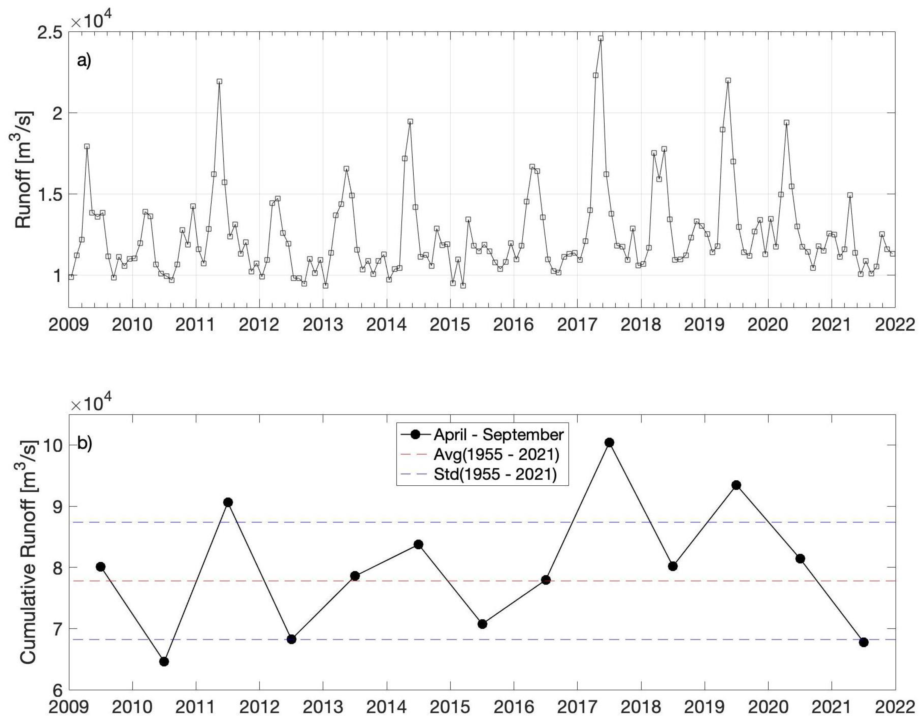
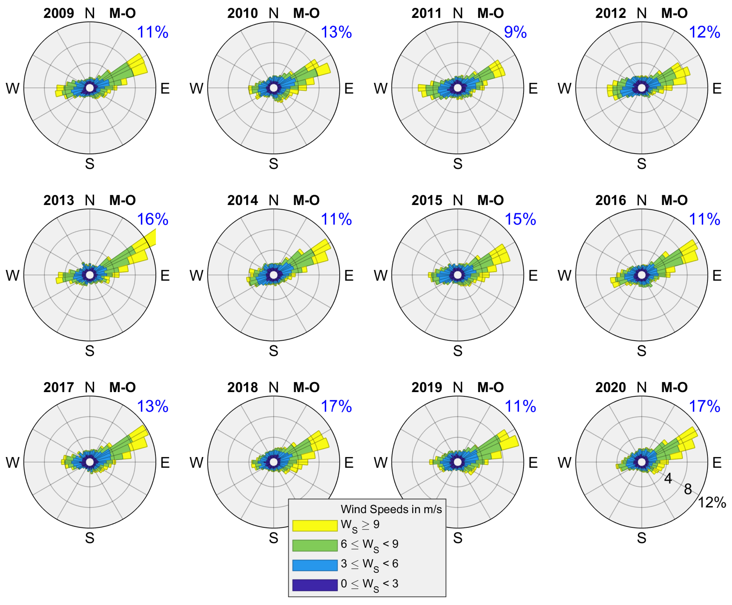
2.2. Freshwater Discharge and Wind Data

Monthly mean estimates of freshwater discharge at the head of the St. Lawrence Estuary near Quebec City are available from the St. Lawrence Global Observatory (SLGO; https://ogsl.ca/en/freshwater-runoffs-quebec-city-application/ (accessed on 1 February 2022)). These runoff data are estimated by an empirical relationship between monthly mean discharge and the monthly mean water level at the Neuville tidal gauge [54]. The annual mean freshwater discharge of the St. Lawrence River at Quebec City shows a similar variation with the sum of all rivers flowing into region of the estuary [55]. Figure 3a shows the monthly river discharge timeseries for the 2009–2021 period. The highest monthly mean runoff of the year is typically in April or May, and in the past two decades, the peak runoff of over 22,000 m${}^3$/s occurred during May in 2011, 2017 and 2019 (Figure 3a). Most years also feature a second, much lower peak river runoff in the late fall, around October. To consider the high runoff of the year and the time taken to reach the nwGSL, the time series of accumulated river discharge from April to September is shown in Figure 3b. Since 2009, accumulated runoff during 2011, 2017, and 2019 has exceeded 90,000 m${}^3$/s, whereas 2010, 2012, and 2021 are low runoff years.

In order to evaluate the impact of wind forcing variability on the current circulation in the nwGSL, the surface zonal and meridional wind components (at 10 m above sea level) are taken from the fifth European Centre for Medium-Range Weather Forecasting Reanalysis (ERA5; Hersbach et al. [56]). The ERA5 is produced using a four-dimensional variational data assimilation scheme with 137 vertical levels and an effective horizontal grid resolution of 31 km. We consider the hourly ERA5 wind analysis at a sampled station near the GC (white square in Figure 1).

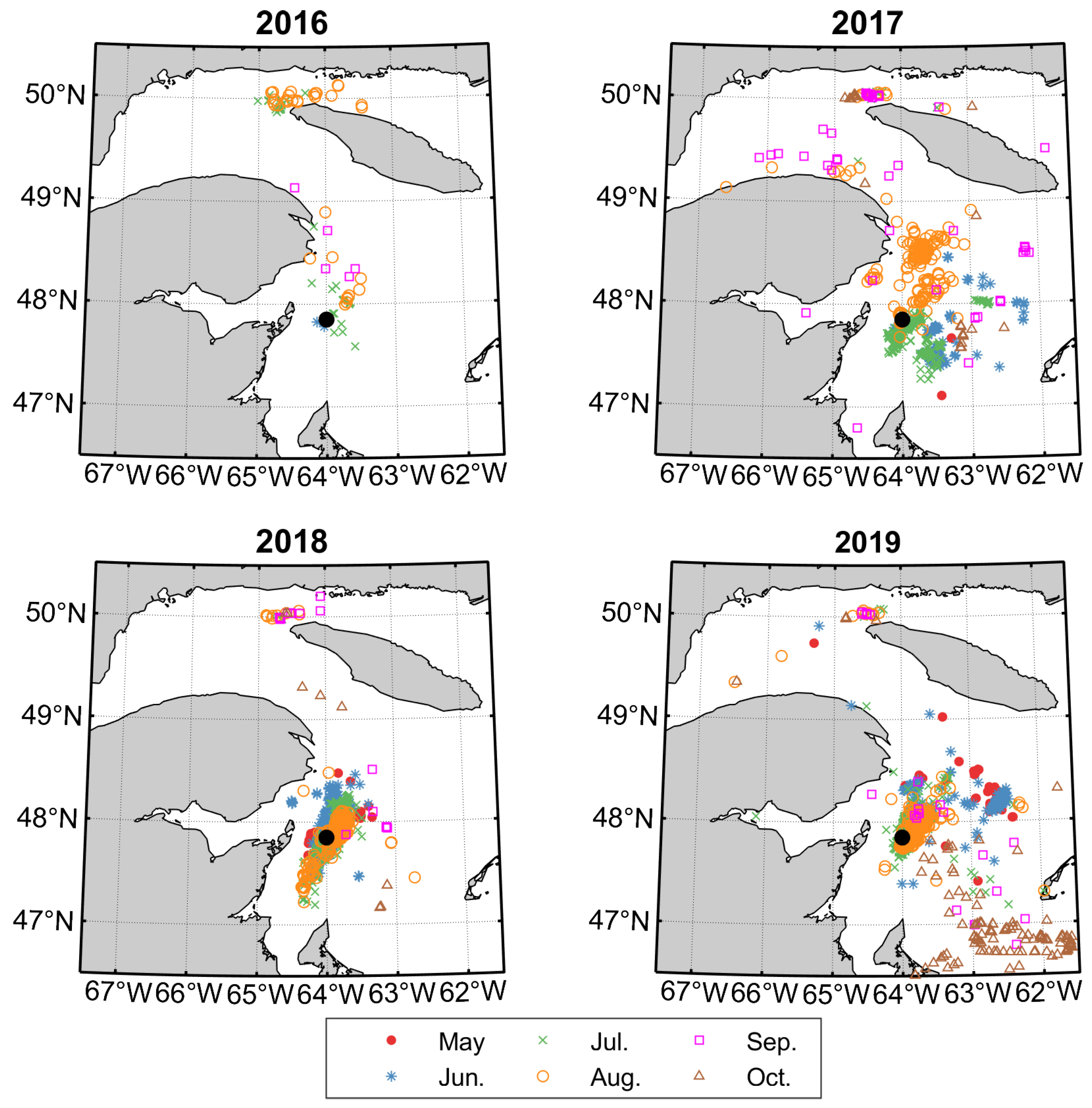
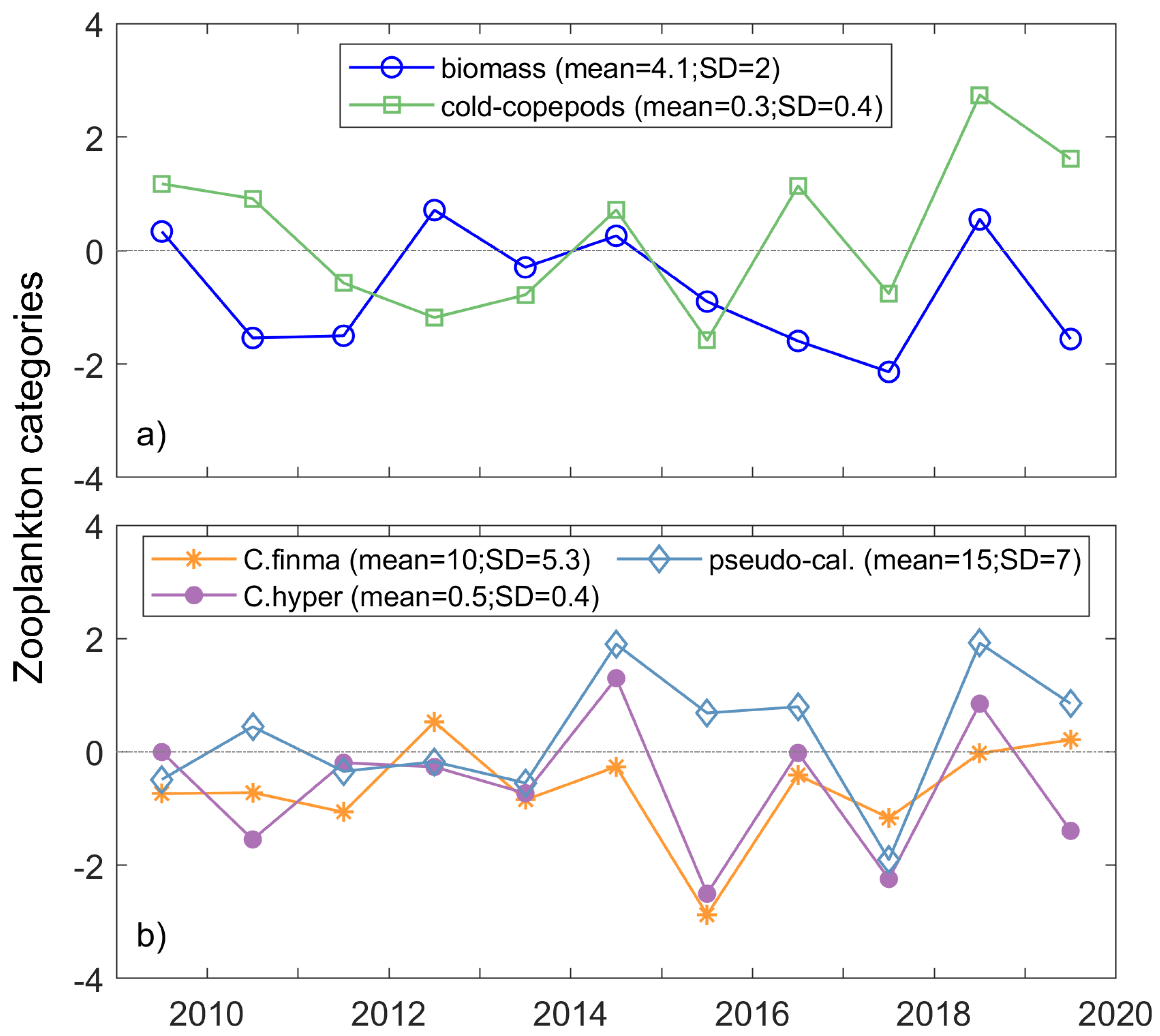
2.3. NARW Sightings and Zooplankton Data

The NARW sighting patterns from 2016 to 2019 are shown in Figure 4, based on combined sightings from North Atlantic Right Whale Consortium [57,58] and DFO (Fisheries and Oceans Canada; DFO [32]) data. Relatively few sightings are apparent in 2016 and May to mid-June 2017, with a large increase in sightings starting in the summer of 2017. This increase in sightings may be at least partially due to the relatively few search efforts that were made in 2016 and early 2017, compared to increased search efforts starting in summer 2017, with systematic cetacean surveys [31,59]. NARW sightings have been largely concentrated in the southern Gulf, in the vicinity of the Shediac Valley station (black dot in Figure 4), where most search efforts have occurred. Although few NARWs have been detected to the northwest of Anticosti Island, search efforts in this area have also been fewer, compared to the southern Gulf, and there is notable variability in NARW sighting distributions during 2017–2019 [31]. During the spring (May and June) of 2017 and 2019, the whales were sighted far from the coast, and were present to the east, in the Shediac Valley along the southern slope of the Laurentian Channel, while whales sightings show a north-south distribution in the Shediac Valley in 2018 (Figure 4). During October 2019, some NARWs were even present between Prince Edward Island and the Magdalen Islands.

It is should be noted that these sighting data may be biased towards areas and times when search efforts have occurred and probably do not represent all NARWs that were present, in all areas and all times. An example is the intensive aerial cetacean survey effort conducted by the DFO and NOAA over this time period [31,60]. These may also include duplicate sightings; e.g., the same animals reported by multiple platforms. Therefore, these data should not be directly interpreted as total number/density of whales over space and time, and lack of sightings in a specific area or during a certain time should not be interpreted as the absence of whales. There are uncertainties and limitations in our understanding of the complete distribution and presence of NARWs in the GSL over time, since systematic surveys tend to be conducted in areas where NARWs are expected to aggregate. Therefore, search effort and survey coverage should also be considered, when interpreting interannual differences in NARW distributions in the sGSL [31].

Blais et al. [36] provide a detailed summary of zooplankton variations along routinely sampled transects and stations in the GSL. All zooplankton sampling and processing steps meet the standards of the Atlantic Zontal Monitoting Program protocol [61], but the sampling methodology slightly changed over time. Figure 5 shows temporal variations in normalized annual anomalies of five different zooplankton indices (total zooplankton biomass, cold-water-associated copepods, Calanus finmarchicus, Calanus hyperboreus and Pseudocalanus) from zooplankton monitoring at the Shediac Valley station, which is embedded within the NARW habitat. This is sampled on a monthly basis between May–November and at a lower frequency during January–April [36]. Zooplankton samples are collected over the entire water column so that these represent depth-integrated zooplankton metrics. The cold-water-associated copepods include two taxa: Metridia longa and Calanus glacialis [36]. Zooplankton anomalies were mostly below normal (anomaly values < 0) during 2011, 2013, and 2017, with a notable drop in all five zooplankton measures in 2017 (Figure 5). The anomaly of Calanus finmarchicus was effectively near-normal from 2014 through 2019, with the exception of a strong decline in 2015.

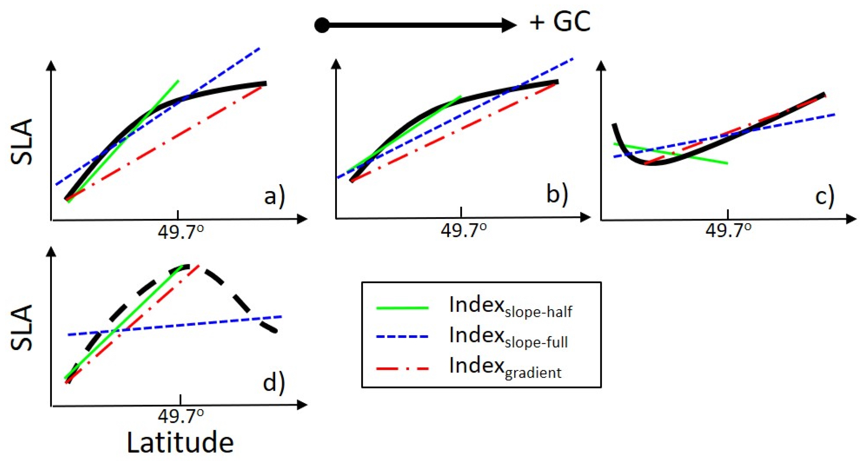
2.4. Altimetric Indices

Satellite altimetry provides a measure of the geostrophic surface currents [44,45,46] via the sea surface height slope relative to the geoid. The u-component ($u_s$) and the v-component ($v_s$) of the geostrophic surface currents can be related to surface elevation $\zeta$ by [46]:

$$u_s=-\frac{g}{f}\frac{\partial \zeta }{\partial y},$$

(1)

$$v_s=\frac{g}{f}\frac{\partial \zeta }{\partial x},$$

(2)

where g is the gravitational constant, and f is the Coriolis parameter. The Jason-2/3 altimeter profiles permit a range of geostrophic current indices to be proposed. We define the slope of SLA along the track (Index${}_{slope}$ in cm/km) as a measure of geostrophic current intensity, where

$$\mathrm{SLA}={\beta }_0+{\mathrm{Index}}_{slope}\times L,$$

(3)

and Index${}_{slope}$ is a linearly regressed coefficient. Here, ${\beta }_0$ is an additive constant and L is the distance of the SLA measurements from the intersection of southern coastline and ground track. Index${}_{slope-full}$ is calculated using a linear fit of the SLA profile along the entire track (49.2${}^{\circ }$ N–50.3${}^{\circ }$ N), as a proxy for the geostrophic current across the Gulf. We also consider Index${}_{slope-half}$ using the southern half of the Jason-2/3 SLA profile, up to the center of the Gulf (49.2${}^{\circ }$ N–49.7${}^{\circ }$ N), which is about 40 km away from the Gaspé Peninsula coastline (Figure 1). This is motivated by variations in the location of the GC, which is known to periodically separate from its typical path around the Gaspé Peninsula [21], and whose width change is about 10–20 km [52].

A third estimate of geostrophic surface current intensity is given by the gradient between the maximum and minimum SLA along a satellite track (Index${}_{gradient}$ in cm/km), as in

$${\mathrm{Index}}_{gradient}=\frac{{\mathrm{SLA}}_{max}-{\mathrm{SLA}}_{min}}{Distanc{e}_{max-min}},$$

(4)

where SLA${}_{max}$ and SLA${}_{min}$ are the maximum and minimum SLA values along the track, respectively, and $Distanc{e}_{max-min}$ is the distance between the corresponding locations. This definition better accommodates a contribution from the Anticosti cyclonic gyre circulation, which is often present in the nwGSL during summer months [23]. We hypothesize that slope index variations (Index${}_{slope}$ and Index${}_{gradient}$) correlate with variations in river discharge, assuming that river discharge dominates the SLA changes.

Figure 6 displays the expected changes in Index${}_{slope-half}$ and Index${}_{gradient}$ as the GC intensity increases. A negative value of Index${}_{slope-half}$ generally indicates a stronger eastward surface current; Index${}_{slope-half}$ values decrease as GC intensity increases (green solid lines in Figure 6). Index${}_{slope-full}$, as derived from the entire SLA profile, is a measure of overall cross-section surface water circulation (blue dashed lines in Figure 6). Index${}_{gradient}$ is defined by the SLA extrema along the entire track and reflects properties of the surface circulation of the Anticosti Gyre (red dash-dotted lines in Figure 6). Index${}_{slope-full}$ and Index${}_{gradient}$ provide complementary characterizations of physical processes in the nwGSL. For example, Index${}_{slope-full}$ displays a weak transport, while the Index${}_{gradient}$ shows a strong current, despite being calculated using the same SLA profile in Figure 6d.

Finally, an altimetric index of volume transport through the track (Index${}_{volume}$ in m × km) can also be considered. We define this as

$${\mathrm{Index}}_{volume}=\frac{{\sum }_{i=1}^n(\frac{SL{A}_i+SL{A}_{i+1}}{2}\times Distanc{e}_{i,i+1})}{n},$$

(5)

where n is the number of along-track values of $SL{A}_i$ and $Distanc{e}_{i,i+1}$ is the distance between available values. We note that data corrections result in some missing measurements along the track, so only the SLA profiles with over 70% of the available data are included in this study.

To visually summarize and compare the interannual variations in an index, a box plot is used [62]. Blais et al. [36] examined the linkage between environmental factors and zooplankton variables using a simple correlation matrix, which shows the Pearson correlation coefficients between different variables. They defined the significant correlations as p-value < 0.1. We use the same method in this study. The Pearson correlation coefficient (R) is used to characterize the strength of the association between two variables.

3. Results

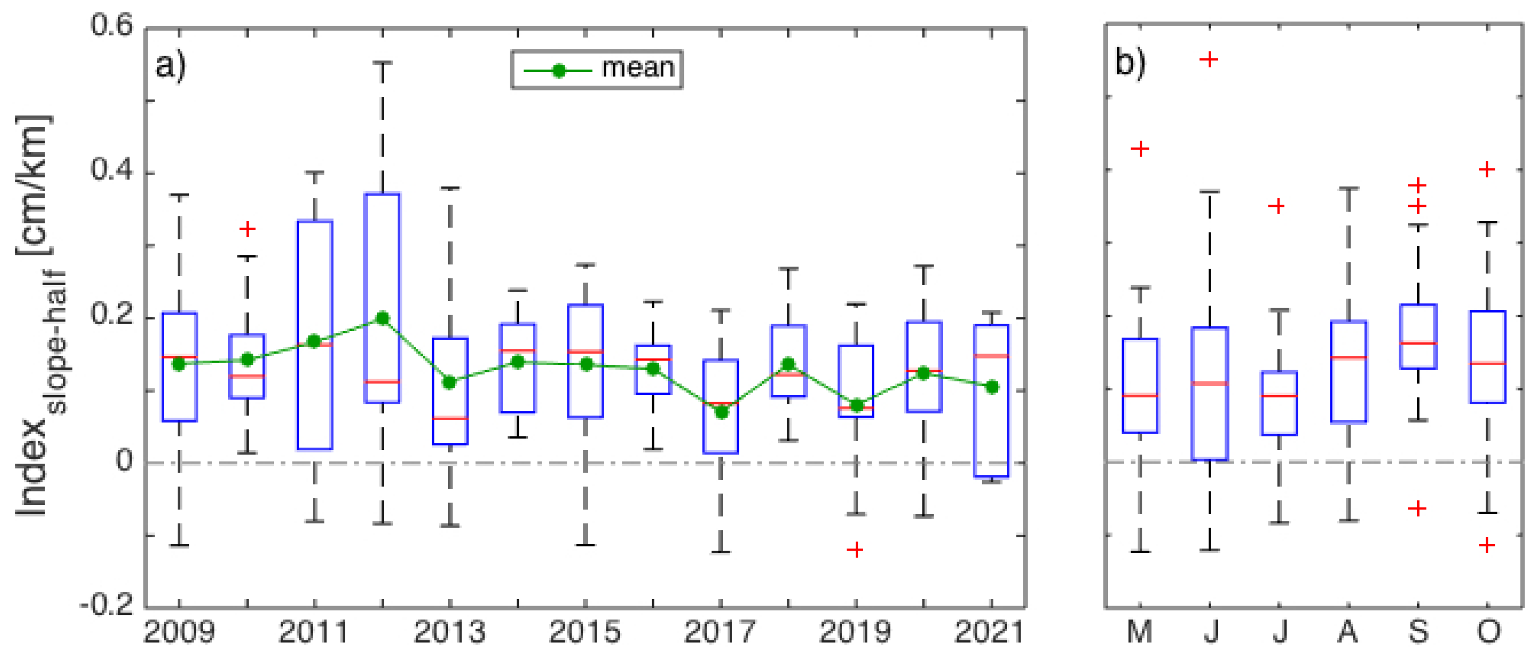
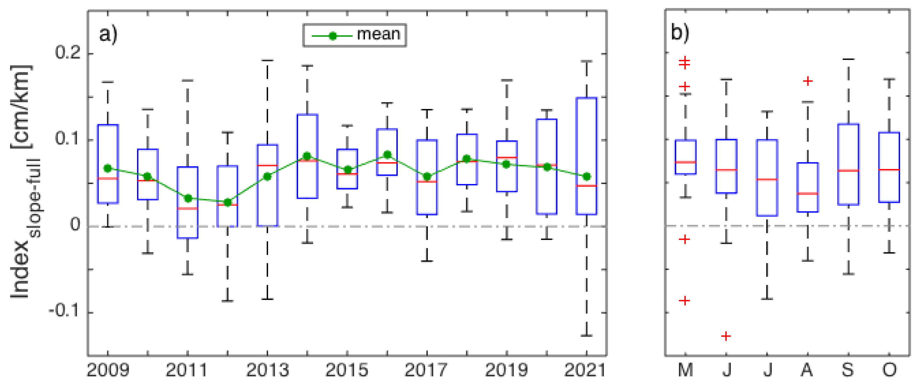
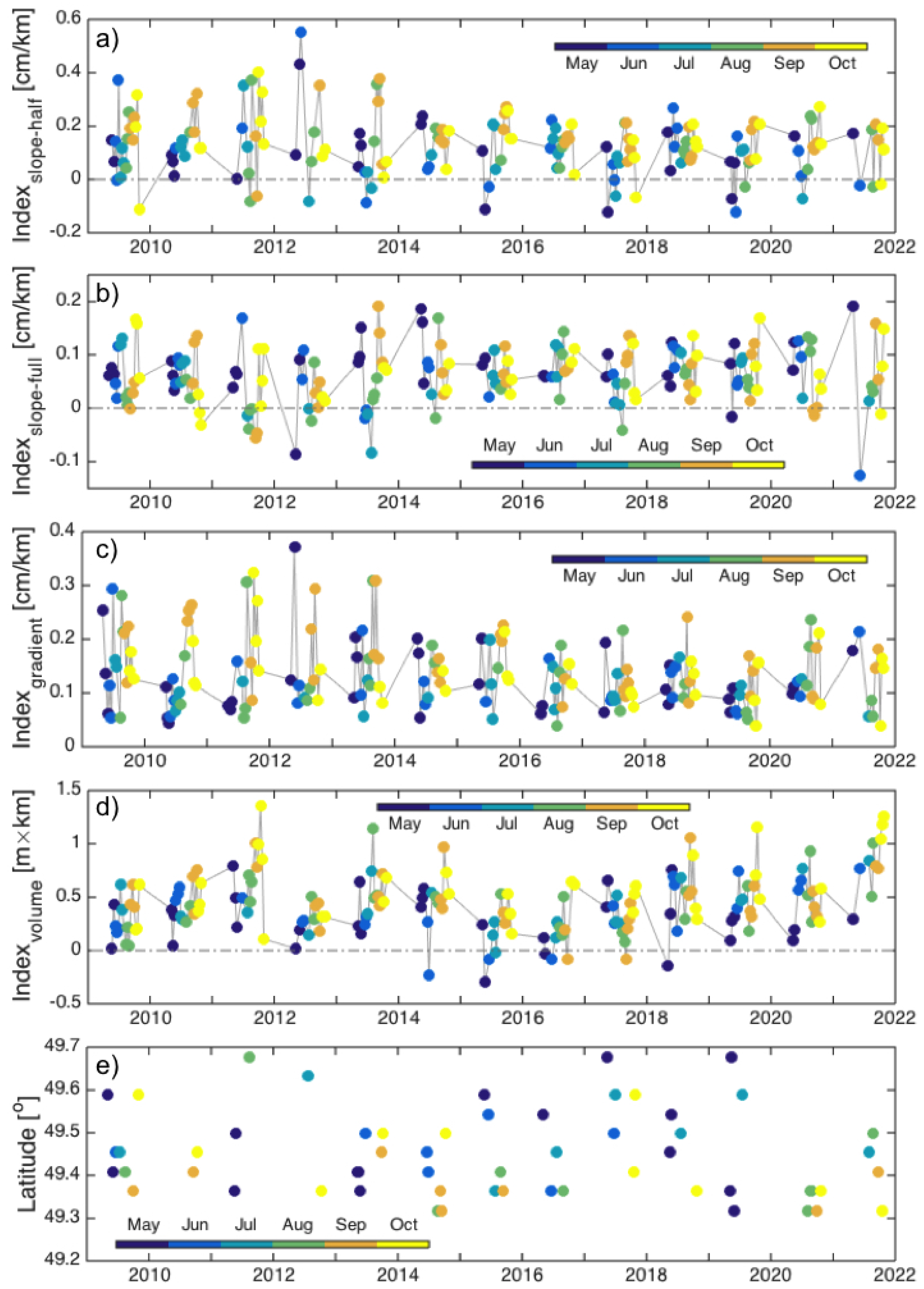
3.1. Interannual Variability in SLA Indices

Three indices have been developed to characterize variations in the GC intensity and extension, surface ocean circulation in the nwGSL, and volume transport across the Gulf, using J2/3 altimetry SLA data from 2009 to 2021. As noted in the previous section, a negative Index${}_{slope}$ [cm/km] indicates a stronger eastward current and a decreasing trend in Index${}_{slope-half}$ indicates an increasing trend in GC intensity. To examine the interannual variation in the Index${}_{slope}$, a box plot analysis was used. Jason-2/3 coverage is fairly evenly distributed throughout each year.

Figure 7 and Figure 8 capture interannual variations in Index${}_{slope-half}$ and Index${}_{slope-full}$. Both median and mean values of Index${}_{slope-half}$ (red line and green dot, respectively, in Figure 7a) were comparatively lower in 2013, 2017 and 2019. The variation in Index${}_{slope-half}$, for the distance between the bottom and top of each box, also known as the interquartile range, was comparatively larger in 2011, 2012 and 2021 (Figure 7a). The monthly Index${}_{slope-half}$ variation is shown in Figure 7b using the data during 2009–2021. Lower Index${}_{slope-half}$ values were observed in May, June and July, and higher Index${}_{slope-half}$ values were observed in August and September, which is consistent with the river discharge variations. Relatively lower Index${}_{slope-half}$ values associated with larger discharge values were observed (Figure 7b). In contrast, the variation in Index${}_{slope-full}$ was comparatively larger during 2009–2014 and 2020–2021, whereas it was relatively smaller during 2015–2019 (Figure 8a). The mean value of Index${}_{slope-full}$ gradually decreased from 2009 to 2012 and then increased in 2013. The mean Index${}_{slope-full}$ varied around 0.075 cm/km during 2013–2020, except in 2017 (Figure 8a). Regarding the monthly Index${}_{slope-full}$ variations, the highest median value was observed in May and the lowest median value was observed in August (Figure 8b).

Index${}_{gradient}$ [cm/km] was calculated using the maximum and minimum values of SLA and corresponding locations along each track. Time series of latitudes for SLA${}_{max}$ and SLA${}_{min}$ were grouped based on month (Figure 9). In general, SLA${}_{max}$ was located on the northern side, and SLA${}_{min}$ was located on the southern side. However, reverse profiles were also observed in each month. The mean location of SLA${}_{max}$ gradually moved southward from May to August. The peak for SLA moved to the center of the Gulf and SLA values decreased outside the center, which indicates a clockwise circulation and surface waters converge in the center. By comparison, SLA${}_{min}$ moved toward the center in May from 2016 to 2019 (Figure 9a), which indicates an anticlockwise circulation and divergent waters at the surface. Additionally, the shortest distance between the mean of SLA${}_{max}$ and SLA${}_{min}$ was found in September (Figure 9d).

As mentioned earlier, Index${}_{gradient}$ is a proxy for the geostrophic velocity across the gyre circulation in the nwGSL, which thereby better accommodates contributions from the Anticosti Gyre (Figure 1). Figure 10a shows the interannual variation in the Index${}_{gradient}$. The variation in Index${}_{gradient}$ was higher in 2011–2015 than in 2016–2019. Additionally, lower Index${}_{gradient}$ values were observed in May, June and July, while higher Index${}_{gradient}$ values were observed in August and September (Figure 10b). Thereafter, Index${}_{gradient}$ values tend to decrease in October. We note that Index${}_{gradient}$ exhibits a similar monthly variation as Index${}_{slope-half}$ (Figure 7b and Figure 10b).

Assuming the location of the SLA${}_{min}$ is influenced by the GC intensity, the SLA${}_{min}$ extends northward (far away from the coastline) when the GC becomes relatively strong. Here, in our study, we remove the SLA profiles from the analysis when SLA${}_{min}$ is located at the south end of the track, or when SLA${}_{min}$ is located further north than 49.7${}^{\circ }$ N (center of the Northwest Gulf). Figure 11a displays the interannual variations in reprocessed SLA${}_{min}$ during 2009–2021. Values for the reprocessed SLA${}_{min}$ were located relatively further north in 2011, 2017 and 2019 (Figure 11a). In addition, the monthly variation in reprocessed SLA${}_{min}$ is displayed in Figure 11b. The median of the SLA${}_{min}$ was located further north in May, when the river discharge reaches its maximum. We note that the median SLA${}_{min}$ is furthest north in July (Figure 11b), which indicates an eastward current in the south and a broader westward current in the north. This agrees with previous studies of a cyclonic gyre in the nwGSL during the summer months [23,25]. The occurrence of SLA${}_{min}$ is located even further north in October and may also be linked to a lower peak river runoff. Most years feature a second peak for river runoff in the late fall, which is much lower than the peak river runoff in the spring (Figure 3a).

The Index${}_{volume}$ [m × km] was calculated using the J2/3 SLA along the entire track (Figure 12a), and it is a proxy for variations in the amount of water flowing through the track. A higher Index${}_{volume}$ indicates a larger amount of water flowing through the track. The Index${}_{volume}$ timeseries for 2009–2021 has strong interannual variations (Figure 12a). Its mean value is generally high during 2009–2014, except for a sudden drop in 2012. From 2015, the Index${}_{volume}$ time series shows a general upwards trend that peaks in 2021 (Figure 12a). Monthly Index${}_{volume}$ values also seem to increase from May to October (Figure 12b).

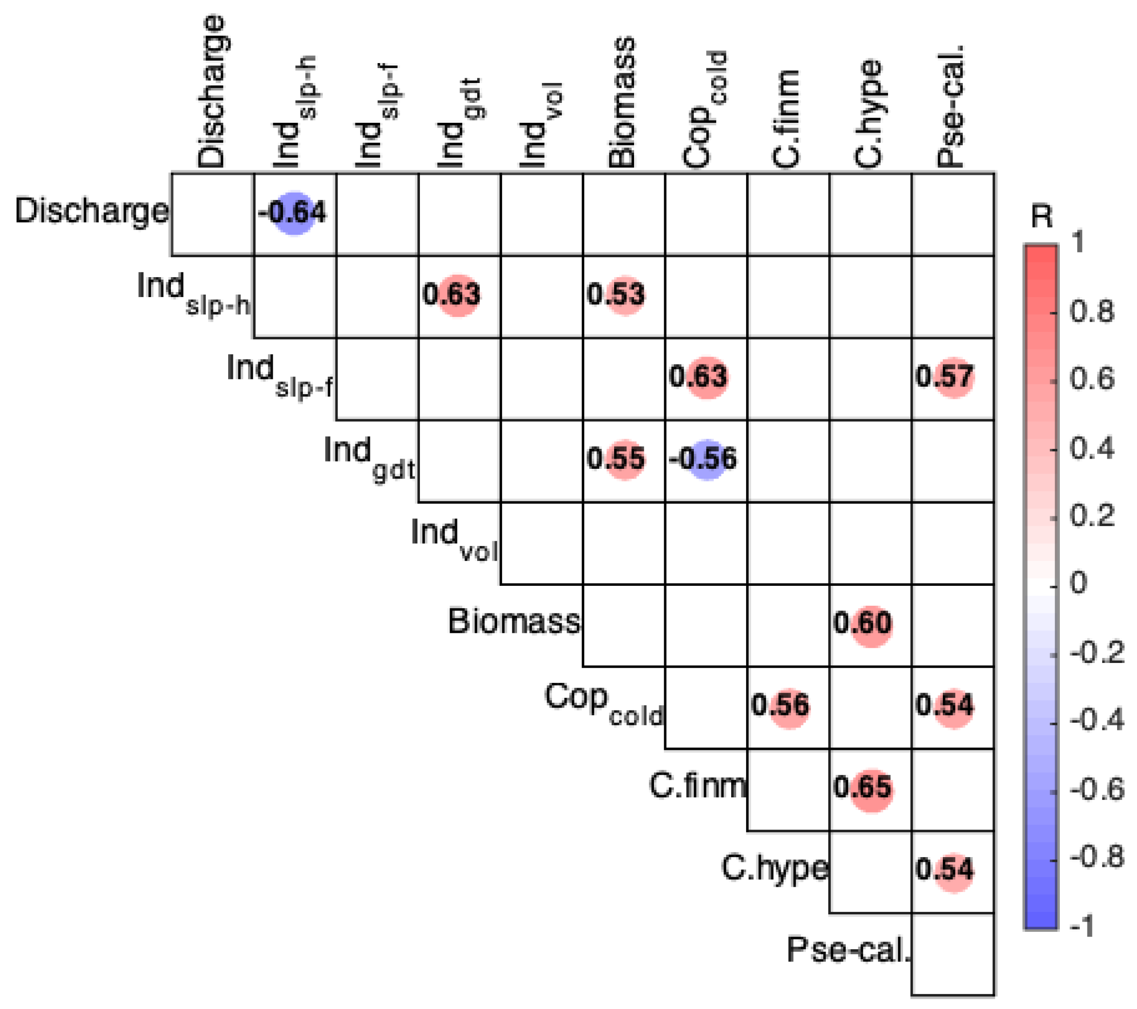
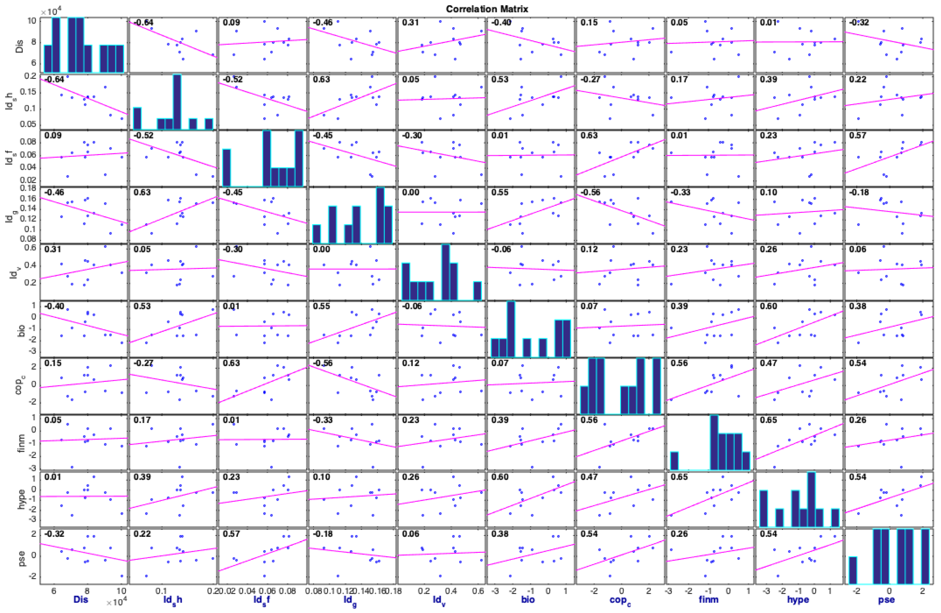
3.2. Correlation Analysis between Physical and Zooplankton Indices

Correlations among discharge, physical indices and zooplankton indices using ‘yearly’ data (2009 to 2019) are examined in Figure 13, with scatterplots given in the Appendix A (Figure A1). Here, discharge is the accumulation of runoff from April to September. Physical indices are annual means using the altimetry data from May to October. Zooplankton indices at the Shediac Valley are the annual anomalies using data mainly collected from May to November. Correlations that were not significant (p-value ≥ 0.1) were removed. The physical values for Index${}_{slope-half}$ show a definite negative correlation with river runoff data (R = −0.64, p-value < 0.05; Figure 13). As Index${}_{slope-half}$ is a proxy for the GC intensity, we suggest that Index${}_{slope-half}$ captures the driving force of the GC due to upstream river runoff. However, although our physical indices are sometimes correlated with zooplankton indices at Shediac Valley, none of the five zooplankton indices are significantly correlated with discharge.

4. Discussion

4.1. Gaspé Current Index Developed from Satellite Altimetry

Physical indices developed from remote sensing data are useful to monitor variations in the strength and extension of the GC, a dominant ocean circulation process in the western GSL. Time series Index${}_{slope-half}$ is negatively correlated with river runoff data. The freshwater discharge appears to dominate stratification and dynamical forcing of the GC [26]. Due to limitations in the resolution of the Jason altimeter and land contamination in altimeter waveforms [63], the Jason-2/3 SLA profiles may not fully capture the entire GC (Figure 2), but SLA profiles still capture the GC variation.

Wind forcing may impact the correlation between Index${}_{slope-half}$ and the river discharge. Based on the variation in discharge, Index${}_{slope-half}$ values are higher than we might expect in 2011 and 2012 (Figure 3 and Figure 7). Koutitonsky and Budgen [21] indicate that wind-stress forcing is also an important source of kinetic energy for the GSL. Lavoie et al. [24] found a correlation between the alongshore (east-west) wind and the surface flow in the nwGSL. The westward alongshore winds cause Ekman transport away from the south coast, a depressed sea level along the south shore, and an increase in Index${}_{slope-half}$. Thus, wind stress can weaken the correlation between river discharge and Index${}_{slope-half}$. Typically, in the nwGSL, the wind most often blows to the east-northeast during May to October, whereas in 2011 and 2012, a stronger westward wind prevailed (Figure 14). Thus, the higher Index${}_{slope-half}$ values in 2011 and 2012 may have been caused by this westward wind component. We noted that small differences from one year to another were observed (Figure 14). Additionally, lower median values of Index${}_{slope-half}$ were found in 2013, 2017 and 2019 (Figure 7a). The river discharge was much larger in 2017 and 2019 than in 2013, while the eastward wind was stronger in 2013. Figure 14 shows that approximately 16% of the time the wind is over 9 m/s and blows to the northeast during the six months sampling period in 2013.

Index${}_{gradient}$ accommodates the surface circulation of the Anticosti Gyre. The expected changes in Index${}_{gradient}$ as the GC intensity increases are shown schematically in Figure 6. Transport at the Strait of Belle Isle along the Quebec North Shore plays an important role in the formation of the cyclonic gyre in the nwGSL [26], while transport at the Cabot Strait through the Laurentian Channel also enhances the circulation in the nwGSL by upwelling and mixing [64]. For fixed volume transport through these openings, the sea level height on the south shore of nwGSL increases as the river discharge increases. SLA${}_{min}$ is generally located on the southern side (Figure 9). If sea level height on the south shore is higher, the SLA gradient between the north and south shore is flattened and Index${}_{gradient}$ is reduced (Figure 6a,b). Index${}_{gradient}$ decreases as the GC intensity increases. In addition, Index${}_{gradient}$ is positively correlated with Index${}_{slope-half}$ (R = −0.63, p-value < 0.05; Figure 13). Furthermore, a stronger GC may also push the SLA${}_{min}$ northward, away from the land (Figure 6c). This variation in the reprocessed SLA${}_{min}$ is broadly consistent with the proposed model. The SLA${}_{min}$ is located relatively further north in high runoff years (2011, 2017 and 2019; Figure 11).

We note that the time series of Index${}_{volume}$ shows an increasing trend during 2015–2021 (Figure 12a), which suggests an increasing volume transport. Previous hydrographic studies highlight several dynamical processes in the nwGSL, such as the outflow from the St. Lawrence Estuary along the north shore of Gaspé Peninsula, wind-induced coastal upwelling along the north shore of nwGSL [21,25], and a barotropic westward jet (Labrador Shelf Current) along the north shore of GSL [26]. However, we find no significant correlation between Index${}_{volume}$ and runoff (Figure 13); one possible explanation is that the transport due to the barotropic westward jet from the Strait of Belle Isle has increased during these years. In addition, the monthly sea surface temperature anomaly over the nwGSL exhibits a generally decreasing trend from 2015 to 2020 [55]. The GSL water is warmer relative to the Labrador Current [65]. Furthermore, Petrie et al. [66] indicated that the net transport through the Strait of Belle Isle toward the GSL is relatively low during summer and high during the winter. This is consistent with the variations in monthly Index${}_{volume}$ (Figure 12b). It is possible that a westward flow affects the relationship between Index${}_{volume}$ and runoff, but this hypothesis requires more research.

4.2. Physical Indices Linked to the Zooplankton Variations

The freshwater volume from the St. Lawrence River controls the GC intensity, which mainly affects the buoyancy-driven circulation, mixing processes and the dynamics of the ecosystem over a wide range of timescales in the GSL (e.g., Koutitonsky and Budgen [21,28]). Phytoplankton are transported to the southern GSL via the GC, which appears to support the production, growth and transport of zooplankton [3,13,41,42]. In the Shediac Valley, Index${}_{slope-half}$, an indicator of GC intensity, is positively correlated with zooplankton biomass in the absence of a correlation between river discharge and biomass. In addition, none of the zooplankton indices are significantly correlated with river discharge (p-value ≥ 0.1; Figure 13). One possible explanation is that altimetric observations capture a range of environmental forcing mechanisms. Thus, the performance of an altimetric index is likely better than a single variable, e.g., river discharge, as an indicator for some zooplankton variations during this period. This result may suggest the use of physical indices developed from satellite observations to infer variations in zooplankton transport.

In this study, the developed physical indices are mainly applicable to zooplankton transport into the sGSL or eastward displacement along the Laurentian Channel slope, which could potentially be related to environmental conditions that affect zooplankton production and growth. However, the performance of an altimetric index as an indicator of zooplankton variations are also affected by the mechanisms responsible for changes in the zooplankton [67]. We note that variations in zooplankton abundance cannot be predicted solely from physical transport processes. Appropriate conditions for zooplankton growth must also occur, and the timing between zooplankton production and advection needs to be properly aligned [3,41,68]. There are sophisticated biogeochemical and grazing mechanisms involved to support the secondary productivity in the GSL. Sorochan et al. [13] has a detailed review on the possible mechanisms driving the zooplankton growth, such as horizontal advection, food availability, and temperature. Brennan et al. [3,38] traced back to the sources of zooplanktons and discussed the evolving process of the zooplanktons in the GSL. They suggested that mechanisms responsible for maintaining high zooplankton stocks in the NARW foraging habitat should be considered in future studies.

In the Shediac Valley, the normalized annual anomaly of Calanus hyperboreus and Pseudocalanus sp., two species of NARWs prey, are correlated with Index${}_{slope-full}$ (R = 0.76 and R = 0.77, respectively; p-value < 0.05) when outliers in 2011 and 2012 are removed (Figure A1). The boxplot method is used for the detection of outliers here. However, altmetric indices are not significantly correlated with the annual variation in the relative abundances of Calanus finmarchicus, another major NARW prey species in the sGSL. Sorochan et al. [13] have shown that the monthly mean in dry weight of Calanus finmarchicus is highest in July–September and Calanus hyperboreus is highest in May–July. The results imply that the linkage between altimetric indices of nwGSL physical processes and downstream zooplankton variations may be broken in specific seasons. Moreover, the relationship between the environmental indicators and zooplankton may change through time [67], and physical indices do not capture all of the relevant processes all of the time.

The normalized annual anomaly of cold-copepods is positively correlated with Index${}_{slope-full}$, negatively correlated with Index${}_{gradient}$ and shows no significant correlation with river discharge (Figure 13). One possible explanation is that Index${}_{slope-full}$ and Index${}_{gradient}$ are physical indices indicating the cross-section surface water circulation in the nwGSL. There are two main noteworthy features in the nwGSL, namely the GC and Anticosti Gyre. Freshwater discharge from the St. Lawrence River drives a surface-intensified eastward flow, which combines with a southward flow from the North Shore to form the eastward-flowing GC. This southward flow is the relatively cold Labrador Shelf Current, which enters the GSL through the Strait of Belle Isle [21,65]. A portion of the GC together with a barotropic westward jet (Labrador Shelf Current) along the Quebec North Shore forms a cyclonic Anticosti Gyre [21,26]. Therefore, Index${}_{slope-full}$ and Index${}_{gradient}$ capture the combined effects of the GC and the Anticosti Gyre. The variation in cold-copepods in the Shediac Valley seems correlated with regional water circulation in the nwGSL. The presence of cold-copepods in the sGSL may act as an indicator of intrusion of the GC deep water into the sGSL.

4.3. Altimetric Indices to Infer Whale Foraging Habitats

GC behavior and circulations in the nwGSL impact the downstream fate of right whale prey [38]. The physical index, Index${}_{slope-half}$, designed to monitor variations in the GC might be useful as a proxy of NARW prey variation and therefore, a potential tool to infer changes in right whale foraging habitat in the sGSL. The GC is a dominant circulation system, acting as a transport pathway for krill and Calanus into the southern GSL [13,41,42]. Moreover, the GC also plays an important role in the advection and horizontal distribution of Calanus in the sGSL [3,38,41]. The GC and its timing relative to late stage Calanus phenology is important, which affects the NARW foraging habitat in the sGSL [38]. The strength and extension of the GC influences the advection of Calanus spp. into the western sGSL or eastward along the Laurentian Channel. In this study, the Index${}_{slope-half}$ values are lower in 2017 and 2019 than in 2018, which indicates that the GC intensity and extension are stronger in 2017 and 2019 (extreme runoff years) than in 2018 (Appendix A, Figure A2a). Direct observations of the whales provide a good indicator to study the whale foraging habitats [13]. There are differences in NARW sighting distributions during 2017–2019 [31]. Based on NARW sighting data (without ‘survey effort’ corrections Figure 4) and whale sightings distributions, as recognized by previous studies (e.g., Crowe et al. [30], DFO [31], Brennan et al. [38]), we found that the variations in Index${}_{slope-half}$ seem broadly consistent with variations in NARW sighting distributions during the spring season (May and June) in 2017–2019. During the spring in 2017 and 2019, whales sightings show an east-west distribution, with a presence to the southeast of Shediac Valley along the southern slope of the Laurentian Channel, while the whale sightings show a north-south distribution in the Shediac Valley in 2018 (Figure 4). Caveats related to these sightings are stated in Section 2.3. In general, strong GC (low values of Index${}_{slope-half}$) seem to shape east-west distributions of whale sightings around the Shediac Valley (in 2017 and 2019), while weak GC (high values of Index${}_{slope-half}$) appear associated with concentrated distributions of whale sightings in the Shediac Valley (in 2018).

However, we note that our understanding of interannual differences in NARW sightings may be influenced by search effort and survey coverage, at fine spatial and temporal scales in the sGSL [31]. Moreover, we only have three years of data for these comparisons. Further studies, including correction of sightings for search effort (e.g., sightings per unit effort), and consistent surveys over multiple years, incorporating models of NARW distributions, based on search effort and improved understanding of the diving and surfacing behavior of NARWs [31], may be needed to more comprehensively investigate interannual variations in NARW distributions in the sGSL in comparison to these physical indexes. Overall, the physical index Index${}_{slope-half}$ may be helpful to capture some variations in the physical circulation in the whale foraging habitat, and could potentially help to simulate spatial and temporal variations in NARW prey transport and aggregation, and thus also, in NARW distributions in the sGSL. Therefore, satellite altimetry provides a unique tool for potential monitoring of the NARW foraging habitat in the GSL.

5. Conclusions

In this study, satellite altimetry is used to capture general circulation variability in the GSL. Physical oceanic circulation is associated with prey availability and supply, which lead to foraging habitat suitability. Therefore, satellite altimetry is a potential tool for studying the ocean dynamics, which can influence zooplankton transport and NARW foraging habitat variability. This study seeks to develop physical indices from nadir altimetric sea level anomaly data to monitor variations in the GC, which is a dominant ocean circulation feature of this region. In this approach, we anticipate that swath coverage from the Surface Water and Ocean Topography (SWOT) mission [69,70], which also offers improved indices of curved flow in gradient balance, may better reveal such links.

The development of nadir altimetric measures and their association with downstream measures of zooplankton abundance and biomass is novel. Index${}_{slope-half}$ reveals the intensity of the GC, and Index${}_{slope-full}$ reveals the overall surface water circulation in the nwGSL. Index${}_{gradient}$ accommodates a contribution from the Anticosti cyclonic gyre circulation. Index${}_{volume}$ is taken as a proxy for variations in volume transport through a cross-section of the nwGSL. The time series of altimetric indices during 2009–2021 exhibit interannual and seasonal environmental variability. Moreover, these altimetric indices capture a range of environmental forcing mechanisms, which are associated with the water and plankton transport by the GC to the sGSL. Results demonstrate that the altimetric index, Index${}_{slope-half}$, is a more direct estimate of the GC intensity than estimates based on the upstream freshwater flow.

This study explored the correlations between the GC altimetric indices and other variables: the runoff of the St. Lawrence River, five zooplankton variables in the Shediac Valley, and the NARW sighting distributions in the sGSL. Index${}_{slope}$ was able to capture the main patterns of the variations in the physical conditions (e.g., ocean circulation features) in the whale habitat ecosystem, and can be potentially used as an indicator of zooplankton abundance transport and the variations in the NARW foraging habitat in the Shediac Valley area. We therefore recommend the use of Index${}_{slope}$ to capture the variations in the circulation processes in the sGSL and potentially for simulation studies of whale foraging habitats.

Additional utility and application of physical indices should be assessed in ongoing research. A modelling approach can be used to test hypotheses of the relationships between these indices and transport in the sGSL. We anticipate that the application of ocean models to simulate SLA could be helpful to forecast GC intrusions into the sGSL and whale foraging habitat changes. Overall, physical indices provide a potential tool for understanding the functioning of the complex sGSL whale habitat ecosystem. This is potentially an important tool for the management of this critically endangered species.

References

1. Cullen, J.J.; Franks, P.J.; Karl, D.M.; Longhurst, A. Physical influences on marine ecosystem dynamics. Sea 2002, 12, 297–336. [Google Scholar]
2. Cox, S.; Embling, C.; Hosegood, P.; Votier, S.; Ingram, S. Oceanographic drivers of marine mammal and seabird habitat-use across shelf-seas: A guide to key features and recommendations for future research and conservation management. Estuar. Coast. Shelf Sci. 2018, 212, 294–310. [Google Scholar] [CrossRef]
3. Brennan, C.E.; Maps, F.; Gentleman, W.C.; Plourde, S.; Lavoie, D.; Chassé, J.; Lehoux, C.; Krumhansl, K.A.; Johnson, C.L. How transport shapes copepod distributions in relation to whale feeding habitat: Demonstration of a new modelling framework. Prog. Oceanogr. 2019, 171, 1–21. [Google Scholar] [CrossRef]
4. Pineda, J.; Starczak, V.; da Silva, J.C.; Helfrich, K.; Thompson, M.; Wiley, D. Whales and waves: Humpback whale foraging response and the shoaling of internal waves at Stellwagen Bank. J. Geophys. Res. Ocean. 2015, 120, 2555–2570. [Google Scholar] [CrossRef]
5. Franks, P.J. Sink or swim: Accumulation of biomass at fronts. Mar. Ecol. Prog. Ser. 1992, 82, 1–12. [Google Scholar] [CrossRef]
6. Pineda, J. Circulation and larval distribution in internal tidal bore warm fronts. Limnol. Oceanogr. 1999, 44, 1400–1414. [Google Scholar] [CrossRef]
7. Epstein, A.W.; Beardsley, R.C. Flow-induced aggregation of plankton at a front: A 2-D Eulerian model study. Deep Sea Res. Part II Top. Stud. Oceanogr. 2001, 48, 395–418. [Google Scholar] [CrossRef]
8. Shanks, A.L.; Wright, W.G. Internal-wave-mediated shoreward transport of cyprids, megalopae, and gammarids and correlated longshore differences in the settling rate of intertidal barnacles. J. Exp. Mar. Biol. Ecol. 1987, 114, 1–13. [Google Scholar] [CrossRef]
9. Lennert-Cody, C.E.; Franks, P.J. Plankton patchiness in high-frequency internal waves. Mar. Ecol. Prog. Ser. 1999, 186, 59–66. [Google Scholar] [CrossRef]
10. Prairie, J.C.; Sutherland, K.R.; Nickols, K.J.; Kaltenberg, A.M. Biophysical interactions in the plankton: A cross-scale review. Limnol. Oceanogr. Fluids Environ. 2012, 2, 121–145. [Google Scholar] [CrossRef]
11. Kingsford, M.; Wolanski, E.; Choat, J. Influence of tidally induced fronts and Langmuir circulations on distribution and movements of presettlement fishes around a coral reef. Mar. Biol. 1991, 109, 167–180. [Google Scholar] [CrossRef]
12. Lavoie, D.; Simard, Y.; Saucier, F.J. Aggregation and dispersion of krill at channel heads and shelf edges: The dynamics in the Saguenay-St. Lawrence Marine Park. Can. J. Fish. Aquat. Sci. 2000, 57, 1853–1869. [Google Scholar] [CrossRef]
13. Sorochan, K.; Brennan, C.E.; Plourde, S.; Johnson, C.L. Availability, supply, and aggregation of prey (Calanus spp.) in foraging areas of the North Atlantic right whale (Eubalaena glacialis). ICES J. Mar. Sci. 2021, 78, 3498–3520. [Google Scholar] [CrossRef]
14. Mayo, C.A.; Marx, M.K. Surface foraging behaviour of the North Atlantic right whale, Eubalaena glacialis, and associated zooplankton characteristics. Can. J. Zool. 1990, 68, 2214–2220. [Google Scholar] [CrossRef]
15. Winn, H.E.; Price, C.A.; Sorensen, P.W. The distributional biology of the right whale (Eubalaena glacialis) in the western North Atlantic. Rep.-Int. Whal. Comm. 1986, 10, 129–138. [Google Scholar]
16. Woodley, T.H.; Gaskin, D.E. Environmental characteristics of North Atlantic right and fin whale habitat in the lower Bay of Fundy, Canada. Can. J. Zool. 1996, 74, 75–84. [Google Scholar] [CrossRef]
17. Abdalla, S.; Kolahchi, A.A.; Ablain, M.; Adusumilli, S.; Bhowmick, S.A.; Alou-Font, E.; Amarouche, L.; Andersen, O.B.; Antich, H.; Aouf, L.; et al. Altimetry for the future: Building on 25 years of progress. Adv. Space Res. 2021, 68, 319–363. [Google Scholar] [CrossRef]
18. Lama, G.F.C.; Sadeghifar, T.; Azad, M.T.; Sihag, P.; Kisi, O. On the indirect estimation of wind wave heights over the southern coasts of Caspian Sea: A comparative analysis. Water 2022, 14, 843. [Google Scholar] [CrossRef]
19. Oziel, L.; Baudena, A.; Ardyna, M.; Massicotte, P.; Randelhoff, A.; Sallée, J.B.; Ingvaldsen, R.B.; Devred, E.; Babin, M. Faster Atlantic currents drive poleward expansion of temperate phytoplankton in the Arctic Ocean. Nat. Commun. 2020, 11, 1705. [Google Scholar] [CrossRef]
20. Cotté, C.; d’Ovidio, F.; Chaigneau, A.; Lévy, M.; Taupier-Letage, I.; Mate, B.; Guinet, C. Scale-dependent interactions of Mediterranean whales with marine dynamics. Limnol. Oceanogr. 2011, 56, 219–232. [Google Scholar] [CrossRef]
21. Koutitonsky, V.G.; Budgen, G. The physical oceanography of the Gulf of St. Lawrence: A review with emphasis on the synoptic variability of the motion. The Gulf St. Lawrence: Small ocean or big estuary? Can. Spec. Publ. Fish. Aquat. Sci. 1991, 113, 57–90. [Google Scholar]
22. Han, G. Sea level and surface current variability in the Gulf of St Lawrence from satellite altimetry. Int. J. Remote Sens. 2004, 25, 5069–5088. [Google Scholar] [CrossRef]
23. Benoit, J.; El-Sabh, M.; Tang, C. Structure and seasonal characteristics of the Gaspé Current. J. Geophys. Res. Ocean. 1985, 90, 3225–3236. [Google Scholar] [CrossRef]
24. Lavoie, D.; Chassé, J.; Simard, Y.; Lambert, N.; Galbraith, P.S.; Roy, N.; Brickman, D. Large-scale atmospheric and oceanic control on krill transport into the St. Lawrence estuary evidenced with three-dimensional numerical modelling. Atmos.-Ocean 2016, 54, 299–325. [Google Scholar] [CrossRef]
25. El-Sabh, M.I. Surface circulation pattern in the Gulf of St. Lawrence. J. Fish. Board Can. 1976, 33, 124–138. [Google Scholar] [CrossRef]
26. Sheng, J. Dynamics of a buoyancy-driven coastal jet: The Gaspe Current. J. Phys. Oceanogr. 2001, 31, 3146–3162. [Google Scholar] [CrossRef]
27. Tang, C. Mixing and circulation in the northwestern Gulf of St. Lawrence: A study of a buoyancy-driven current system. J. Geophys. Res. Ocean. 1980, 85, 2787–2796. [Google Scholar] [CrossRef]
28. Ohashi, K.; Sheng, J. Influence of St. Lawrence River discharge on the circulation and hydrography in Canadian Atlantic waters. Cont. Shelf Res. 2013, 58, 32–49. [Google Scholar] [CrossRef]
29. Lehoux, C.; Plourde, S.; Lesage, V. Significance of Dominant Zooplankton Species to the North Atlantic Right Whale Potential Foraging Habitats in the Gulf of St. Lawrence: A Bio-Energetic Approach; Canadian Science Advisory Secretariat (CSAS) 2020, 2020/033, vi+44p. Available online: https://epe.lac-bac.gc.ca/100/201/301/weekly_acquisitions_list-ef/2020/20-35/publications.gc.ca/collections/collection_2020/mpo-dfo/fs70-5/Fs70-5-2020-033-eng.pdf (accessed on 2 February 2022).
30. Crowe, L.M.; Brown, M.W.; Corkeron, P.J.; Hamilton, P.K.; Ramp, C.; Ratelle, S.; Vanderlaan, A.S.; Cole, T.V. In plane sight: A mark-recapture analysis of North Atlantic right whales in the Gulf of St. Lawrence. Endanger. Species Res. 2021, 46, 227–251. [Google Scholar] [CrossRef]
31. DFO. Updated Information on the Distribution of North Atlantic Right Whale in Canadian Waters. Canadian Science Advisory Secretariat (CSAS). Science Advisory Report 2020/037. 2020. Available online: https://waves-vagues.dfo-mpo.gc.ca/library-bibliotheque/40938554.pdf (accessed on 2 February 2022).
32. DFO. Whalesightings Database; Team Whale, Fisheries and Oceans Canada: Dartmouth, NS, Canada, 2022. [Google Scholar]
33. Durette-Morin, D.; Evers, C.; Johnson, H.D.; Kowarski, K.; Delarue, J.; Moors-Murphy, H.; Maxner, E.; Lawson, J.W.; Davies, K.T. The distribution of North Atlantic right whales in Canadian waters from 2015–2017 revealed by passive acoustic monitoring. Front. Mar. Sci. 2022, 9, 976044. [Google Scholar] [CrossRef]
34. Simard, Y.; Roy, N.; Giard, S.; Aulanier, F. North Atlantic right whale shift to the Gulf of St. Lawrence in 2015, revealed by long-term passive acoustics. Endanger. Species Res. 2019, 40, 271–284. [Google Scholar] [CrossRef]
35. Gavrilchuk, K.; Lesage, V.; Fortune, S.; Trites, A.; Plourde, S. A Mechanistic Approach to Predicting Suitable Foraging Habitat for Reproductively Mature North Atlantic Right Whales in the Gulf of St. Lawrence; Canadian Science Advisory Secretariat (CSAS): Ottawa, ON, Canada, 2020; Volume 2020/034, Available online: https://publications.gc.ca/site/eng/9.890978/publication.html (accessed on 2 February 2022).
36. Blais, M.; Galbraith, P.; Plourde, S.; Devine, L.; Lehoux, C. Chemical and Biological Oceanographic Conditions in the Estuary and Gulf of St. Lawrence during 2019; DFO Canadian Science Advisory Secretariat Research Document; Canadian Science Advisory Secretariat: Ottawa, ON, Canada, 2021; Volume 2021/002, p. iv + 66. Available online: https://publications.gc.ca/site/eng/9.896897/publication.html (accessed on 31 August 2023).
37. Conover, R. Comparative life histories in the genera Calanus and Neocalanus in high latitudes of the northern hemisphere. Hydrobiologia 1988, 167, 127–142. [Google Scholar] [CrossRef]
38. Brennan, C.E.; Maps, F.; Gentleman, W.C.; Lavoie, D.; Chassé, J.; Plourde, S.; Johnson, C.L. Ocean circulation changes drive shifts in Calanus abundance in North Atlantic right whale foraging habitat: A model comparison of cool and warm year scenarios. Prog. Oceanogr. 2021, 197, 102629. [Google Scholar] [CrossRef]
39. Plourde, S.; Lehoux, C.; Johnson, C.; Perrin, G.; Lesage, V. North Atlantic right whale (Eubalaena glacialis) Its Food: A (I) spatial climatology of Calanus biomass and new potential foraging habitats in Canadian waters. J. Plankton Res. 2019, 41, 667–685. [Google Scholar] [CrossRef]
40. Sorochan, K.; Brennan, C.E.; Plourde, S.; Johnson, C.L. Spatial variation and transport of abundant copepod taxa in the southern Gulf of St. Lawrence in autumn. J. Plankton Res. 2021, 43, 908–926. [Google Scholar] [CrossRef]
41. Maps, F.; Zakardjian, B.A.; Plourde, S.; Saucier, F.J. Modeling the interactions between the seasonal and diel migration behaviors of Calanus finmarchicus and the circulation in the Gulf of St. Lawrence (Canada). J. Mar. Syst. 2011, 88, 183–202. [Google Scholar] [CrossRef]
42. Benkort, D.; Lavoie, D.; Plourde, S.; Dufresne, C.; Maps, F. Arctic and Nordic krill circuits of production revealed by the interactions between their physiology, swimming behaviour and circulation. Prog. Oceanogr. 2020, 182, 102270. [Google Scholar] [CrossRef]
43. Plourde, S.; Runge, J.A. Reproduction of the planktonic copepod Calanus finmarchicus in the Lower St. Lawrence Estuary: Relation 682 to the cycle of phytoplankton production and evidence for a Calanus pump. Mar. Ecol. Prog. Ser. 1993, 102, 217–227. [Google Scholar] [CrossRef]
44. Fu, L.L.; Chelton, D.B. Large-scale ocean circulation. In International Geophysics; Elsevier: Berlin/Heidelberg, Germany, 2001; Volume 69, pp. 133–169, iii–viii. [Google Scholar] [CrossRef]
45. Bonjean, F.; Lagerloef, G.S. Diagnostic model and analysis of the surface currents in the tropical Pacific Ocean. J. Phys. Oceanogr. 2002, 32, 2938–2954. [Google Scholar] [CrossRef]
46. Yu, Y.; Wang, L.; Li, Z.; Zhou, X. Geostrophic current estimation using altimetric cross-track method in northwest Pacific Ocean. In IOP Conference Series: Earth and Environmental Science; IOP Publishing: Bristol, UK, 2014; Volume 17, p. 012105. [Google Scholar]
47. Joseph, A. Measuring Ocean Currents: Tools, Technologies, and Data; Elsevier: Amsterdam, The Netherlands, 2013. [Google Scholar]
48. Han, G.; Tang, C.; Smith, P. Annual variations of sea surface elevation and currents over the Scotian Shelf and slope. J. Phys. Oceanogr. 2002, 32, 1794–1810. [Google Scholar] [CrossRef]
49. Rio, M.H.; Mulet, S.; Picot, N. Beyond GOCE for the ocean circulation estimate: Synergetic use of altimetry, gravimetry, and in situ data provides new insight into geostrophic and Ekman currents. Geophys. Res. Lett. 2014, 41, 8918–8925. [Google Scholar] [CrossRef]
50. Mertz, G.; El-Sabh, M.I.; Proulx, D.; Condal, A.R. Instability of a buoyancy-driven coastal jet: The Gaspé Current and its St. Lawrence precursor. J. Geophys. Res. Ocean. 1988, 93, 6885–6893. [Google Scholar] [CrossRef]
51. Mertz, G.; El-sabh, M.I. An Autumn Instability Event in the Gaspé: Current. J. Phys. Oceanogr. 1989, 19, 148–156. [Google Scholar] [CrossRef]
52. Lavoie, D.; Starr, M.; Zakardjian, B.; Larouche, P. Identification of Ecologically and Biologically Significant Areas (EBSA) in the Estuary and Gulf of St. Lawrence: Primary Production; Fisheries and Oceans: Langley, BC, Canada, 2008.
53. Bugden, G. Freshwater runoff effects in the marine environment: The Gulf of St Lawrence example. Can. Tech. Rep. Fish. Aquat. Sci. 1982, 1078, 1–89. [Google Scholar]
54. Bourgault, D.; Koutitonsky, V.G. Real-time monitoring of the freshwater discharge at the head of the St. Lawrence Estuary. Atmos.-Ocean 1999, 37, 203–220. [Google Scholar] [CrossRef]
55. Galbraith, P.; Chassé, J.; Shaw, J.-L.; Dumas, J.; Caverhill, C.; Lefaivre, D.; Lafleur, C. Physical Oceanographic Conditions in the Gulf of St. Lawrence during 2020; Canadian Science Advisory Secretariat: Ottawa, ON, Canada, 2021; Volume 2021/045, pp. 1919–5044. Available online: https://publications.gc.ca/site/eng/9.900562/publication.html (accessed on 2 February 2022).
56. Hersbach, H.; Bell, B.; Berrisford, P.; Hirahara, S.; Horányi, A.; Muñoz-Sabater, J.; Nicolas, J.; Peubey, C.; Radu, R.; Schepers, D.; et al. The ERA5 global reanalysis. Q. J. R. Meteorol. Soc. 2020, 146, 1999–2049. [Google Scholar] [CrossRef]
57. Kenney, R.D. The North Atlantic Right Whale Consortium Database: A Guide for Users and Contributors. 2019. Available online: https://www.narwc.org/uploads/1/1/6/6/116623219/narwc_users_guide__v_6_.pdf (accessed on 2 February 2022).
58. NARWC. Identification and Sightings Data of the North Atlantic Right Whale Consortium as of January 2021; New England Aquarium: Boston, MA, USA, 2021. [Google Scholar]
59. DFO. Review of North Atlantic Right Whale Occurrence and Risk of Entanglements in Fishing Gear and Vessel Strikes in Canadian Waters; Canadian Science Advisory Secretariat: Ottawa, ON, Canada, 2019; Volume 2019/028, Available online: https://publications.gc.ca/site/eng/9.875486/publication.html (accessed on 2 February 2022).
60. Cole, T.V.; Crowe, L.M.; Corkeron, P.J.; Vanderlaan, A.S. North Atlantic Right Whale Abundance, Demography and Residency in the Southern Gulf of St. Lawrence Derived from Directed Aerial Surveys. Canadian Science Advisory Secretariat, 2020/063. 2020. Available online: https://publications.gc.ca/site/eng/9.901892/publication.html (accessed on 2 February 2022).
61. Mitchell, M.R.; Harrison, G.; Pauley, K.; Gagné, A.; Maillet, G.; Strain, P. Atlantic Zontal Monitoting Program Sampling Protocol. In Canadian Technical Report of Hydrography and Ocean Sciences; Fisheries & Oceans Canada, Maritimes Region, Ocean Sciences Division, Bedford Institute of Oceanography: Dartmouth, NS, Canada, 2002; Volume 223, Available online: https://publications.gc.ca/site/eng/9.562291/publication.html (accessed on 2 February 2022).
62. Williamson, D.F.; Parker, R.A.; Kendrick, J.S. The box plot: A simple visual method to interpret data. Ann. Intern. Med. 1989, 110, 916–921. [Google Scholar] [CrossRef]
63. Halimi, A.; Mailhes, C.; Tourneret, J.Y.; Thibaut, P.; Boy, F. Parameter estimation for peaky altimetric waveforms. IEEE Trans. Geosci. Remote Sens. 2012, 51, 1568–1577. [Google Scholar] [CrossRef]
64. Bobanović, J.; Thompson, K.R. The influence of local and remote winds on the synoptic sea level variability in the Gulf of Saint Lawrence. Cont. Shelf Res. 2001, 21, 129–144. [Google Scholar] [CrossRef]
65. Neu, H.J.A. Man-made changes–The potential benefits and liabilities. In Bedford Institute, Gulf of St Lawrence Workshop; Bedford Institute of Oceanography: Dartmouth, NS, Canada, 1968; pp. 75–77. [Google Scholar]
66. Petrie, B.; Toulany, B.; Garrett, C. The transport of water, heat and salt through the Strait of Belle Isle. Atmos.-Ocean 1988, 26, 234–251. [Google Scholar] [CrossRef]
67. Hare, J.A.; Kane, J. Zooplankton of the Gulf of Maine—A changing perspective. In American Fisheries Society Symposium; American Fisheries Society: Bethesda, MD, USA, 2012; Volume 79, pp. 115–137. [Google Scholar]
68. Zakardjian, B.A.; Sheng, J.; Runge, J.A.; McLaren, I.; Plourde, S.; Thompson, K.R.; Gratton, Y. Effects of temperature and circulation on the population dynamics of Calanus finmarchicus in the Gulf of St. Lawrence and Scotian Shelf: Study with a coupled, three-dimensional hydrodynamic, stage-based life history model. J. Geophys. Res. Ocean. 2003, 108. [Google Scholar] [CrossRef]
69. Morrow, R.; Fu, L.L.; Ardhuin, F.; Benkiran, M.; Chapron, B.; Cosme, E.; d’Ovidio, F.; Farrar, J.T.; Gille, S.T.; Lapeyre, G.; et al. Global observations of fine-scale ocean surface topography with the Surface Water and Ocean Topography (SWOT) mission. Front. Mar. Sci. 2019, 6, 232. [Google Scholar] [CrossRef]
70. Han, G.; Perrie, W.; Hannah, C.; Bianucci, L.; Grisouard, N.; Straub, D.; Klymak, J.; Smith, G.; Matte, P. Integration of SWOT Measurements in Canadian Oceanographic Research and Operation. Surface Water and Ocean Topography (SWOT) Mission Document. 2020. Available online: https://swot.jpl.nasa.gov/system/documents/files/4175_SWOT_Canada_Project_Summary.pdf?list=projects (accessed on 2 February 2022).
Figure 1. Bathymetry of the western Gulf of St. Lawrence (GSL, black dashed box) and portion of a repeating Jason-2/3 ground track (black line). The red box in the upper inset shows the location of the GSL. Locations of a wind speed analysis gridbox and the Shediac Valley (SV) biological sampling station (see text) are shown by a white square and black dot, respectively. Gray arrows denote the larger-scale circulation and the black dashed curve represents a fully extended Gaspé Current front. Other acronyms are AI for Anticosti Island, SBI for Strait of Belle Isle and MI for Magdalen Islands. The northwestern GSL (nwGSL) indicates the area between the north shore of the Gaspé Peninsula and the north shore of the GSL.
Jmse 11 01760 g001
Figure 2. Histogram of distance between the Gaspé Peninsula coastline and the southernmost valid SLA value, as a fraction of available J2/3 profiles between 2009 and 2021.
Jmse 11 01760 g002
Figure 3. Time series of the St. Lawrence River (a) monthly runoff from 2009 to 2021 and (b) accumulated runoff during April to September.
Jmse 11 01760 g003
Figure 4. North Atlantic Right Whale (NARW) pattern distributions from 2016 to 2019 using combined sightings (see text). The black dot indicates the Shediac Valley station. Different symbols correspond to whale sightings observed in different months as indicated in the bottom panel. Note that there were few systematic cetacean surveys conducted in 2016 and during May to mid-June 2017.
Jmse 11 01760 g004
Figure 5. Temporal variations in zooplankton presence at the Shediac Valley station (black dot in Figure 1). The five indices are normalized annual anomalies of (a) total zooplankton biomass (dry weight, g/m 2 ) and abundance (×10 3  ind/m 2 ) of cold-water-associated copepods, (b) Calanus finmarchicus, Calanus hyperboreus and Pseudocalanus. Anomalies are given relative to means for the 1999–2015 reference period as shown in the legend. A horizontal dashed line marks the 0 demarcation. Note that copepod presence is somewhat low in 2017 and 2019 (digitized from Blais et al. [36]).
Jmse 11 01760 g005
Figure 6. Schematic diagram illustrates how Index s l o p e h a l f  (green solid line), Index s l o p e f u l l  (blue dashed line) and Index g r a d i e n t  (red dash-dotted line) respond to changes in latitudinal distributions of SLA (black solid curve) when the GC is (a) weak, (b) medium, and (c) strong. (d) The black dashed curve represents different latitudinal distributions of SLA.
Jmse 11 01760 g006
Figure 7. (a) Box plot time series showing the variability in Index s l o p e h a l f  derived from J2/3 SLA profiles to 49.7  N from 2009 to 2021. Green dots are the mean values of Index s l o p e h a l f  in each year. (b) Box plot time series showing the monthly variability in Index s l o p e h a l f . The bottom and top of each box (Q1 and Q3) are the 25th and 75th percentiles of the index in each year, respectively. The distance between the bottom and top of each box is the interquartile range (IQR). The red line in the middle of each box is the median. The dashed line extending above and below each box is a whisker, which goes from the end of the IQR to furthest observation within the whisker length (1.5 × IQR). The red ‘+’ markers are outliers which denote data that fall outside of this interval, defined by Q1 − 1.5 × IQR to Q3 + 1.5 × IQR.
Jmse 11 01760 g007
Figure 8. (a) Box plot time series showing the variability in Index s l o p e f u l l  derived from J2/3 SLA profiles to 50.3  N from 2009 to 2021. Green dots are the mean values of Index s l o p e f u l l  in each year. (b) Box plot time series showing the monthly variability in Index s l o p e f u l l . Note that the ordinate range is reduced.
Jmse 11 01760 g008
Figure 9. The time series of the latitude of SLA m a x  (blue dotted line) and SLA m i n  (black squared line) derived from J2/3 profiles, which have been grouped on (a) May, (b) June, (c) July, (d) August, (e) September, and (f) October. The dashed lines are the respective means for 2009–2021.
Jmse 11 01760 g009
Figure 10. (a) Box plot time series showing the variability in Index g r a d i e n t  derived from J2/3 SLA profiles from 2009 to 2021. Green dots are the mean values of Index g r a d i e n t  in each year. (b) Box plot time series showing the monthly variability in Index g r a d i e n t , from May to October.
Jmse 11 01760 g010
Figure 11. (a) Box plot time series displaying the SLA m i n  interannual variation during the period from 2009 to 2021. Green dots are the mean values of SLA m i n  in each year. (b) Box plots displaying the monthly SLA m i n  variation.
Jmse 11 01760 g011
Figure 12. (a) Box plot time series showing the variability in Index v o l u m e  derived from J2/3 SLA profile up to 50.3  N from 2009 to 2021. Green dots are the mean values of Index v o l u m e  in each year. (b) Box plot time series showing the monthly variability in Index v o l u m e  from May to October. A horizontal dashed line marks the 0 demaraction.
Jmse 11 01760 g012
Figure 13. Correlations among discharge, physical indices and zooplankton indices using yearly data from 2009 to 2019. The correlation coefficients (R) are colored by value. Correlations that are not significant (p-value ≥ 0.1) are removed. Here, we use the following abbreviations: Ind s l p h —Index s l o p e  derived from profiles up to 49.7  N; Ind s l p f —Index s l o p e  derived from profiles up to 50.3  N; Ind g d t —Index g r a d i e n t ; Ind v o l —Index v o l u m e  derived from profiles up to 50.3  N; Cop c o l d —cold-water-associated copepods; C. finm—Calanus finmarchicus; C. hype—Calanus hyperboreus; Pse-cal—Pseudocalanus spp.
Jmse 11 01760 g013
Figure 14. Wind rose patterns showing the distributions of ERA5 hourly wind speed and direction from May to October during 2009–2020 at the sampling station (white square in Figure 1). The percentage (%) of time with strong eastward wind (>9 m/s) during the sampling period is labeled in each panel.
Jmse 11 01760 g014
Disclaimer/Publisher’s Note: The statements, opinions and data contained in all publications are solely those of the individual author(s) and contributor(s) and not of MDPI and/or the editor(s). MDPI and/or the editor(s) disclaim responsibility for any injury to people or property resulting from any ideas, methods, instructions or products referred to in the content.