
Error Evolutions and Analyses on Joint Effects of SST and SL via Intermediate Coupled Models and Conditional Nonlinear Optimal Perturbation Method

Abstract
:1. Introduction
2. Model and Methods
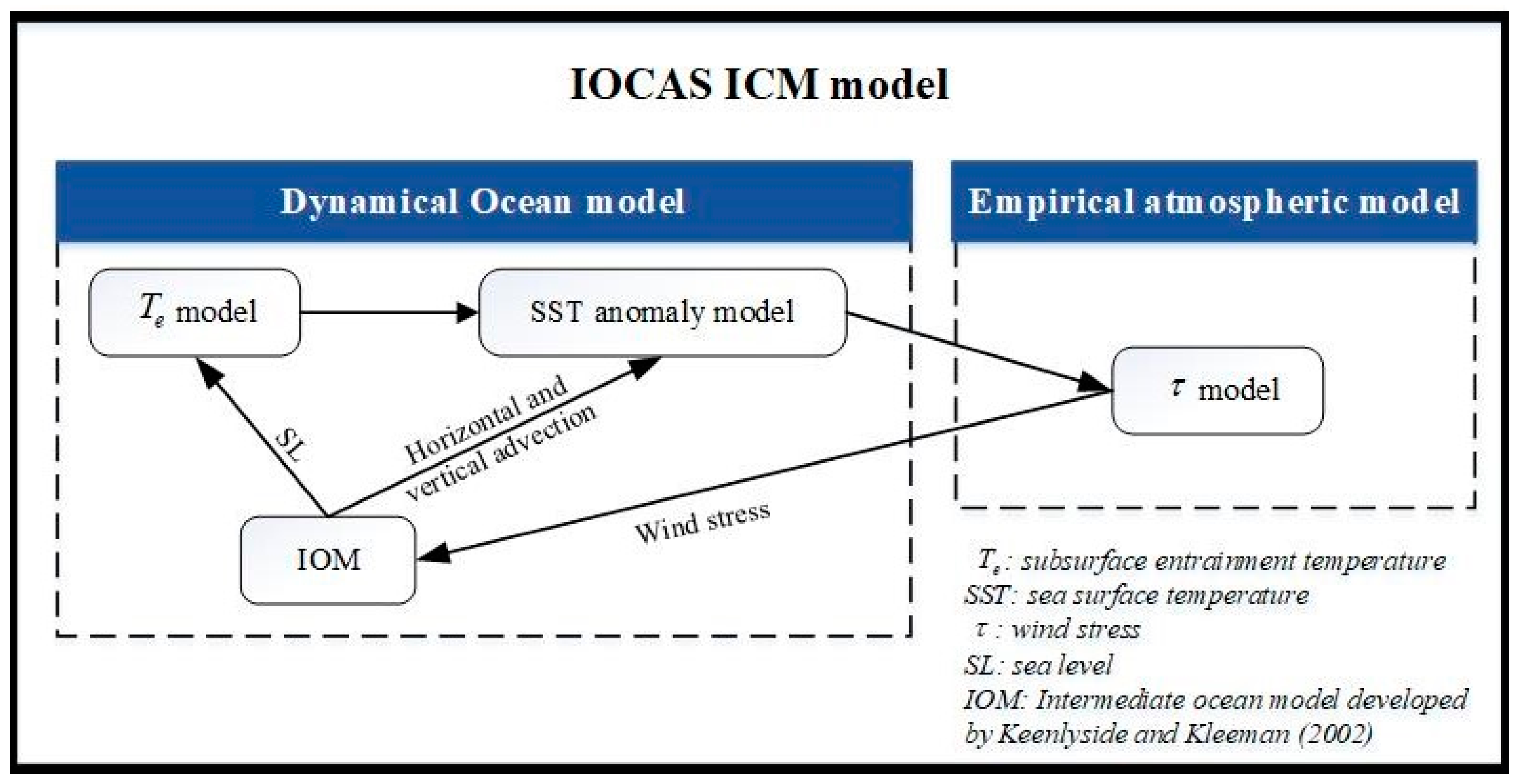
2.1. IOCAS ICM
2.2. CNOP Method
2.3. Solving CNOP of ICM with GD Algorithm
3. Experimental Schema
4. Result Analyses
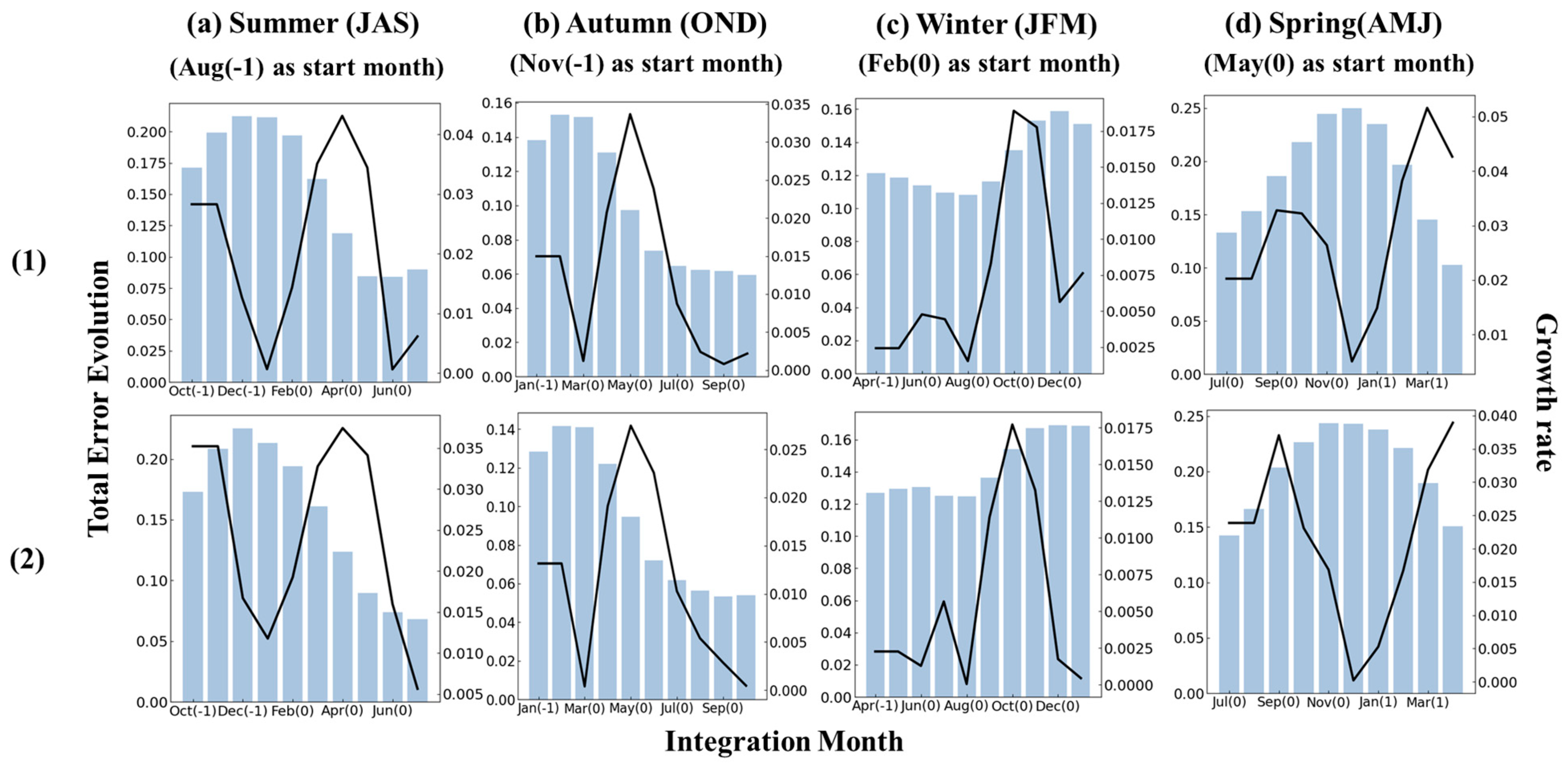
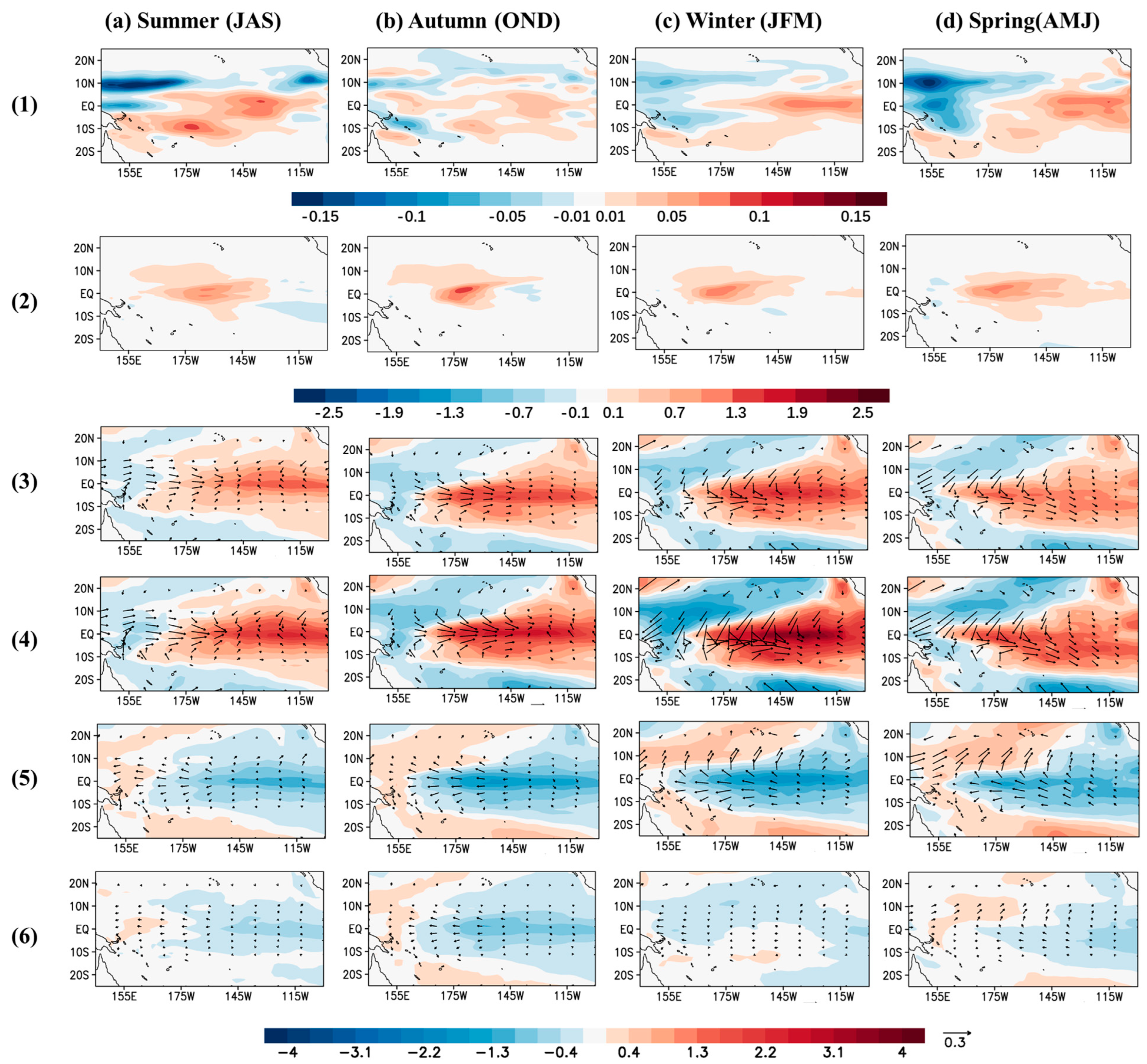
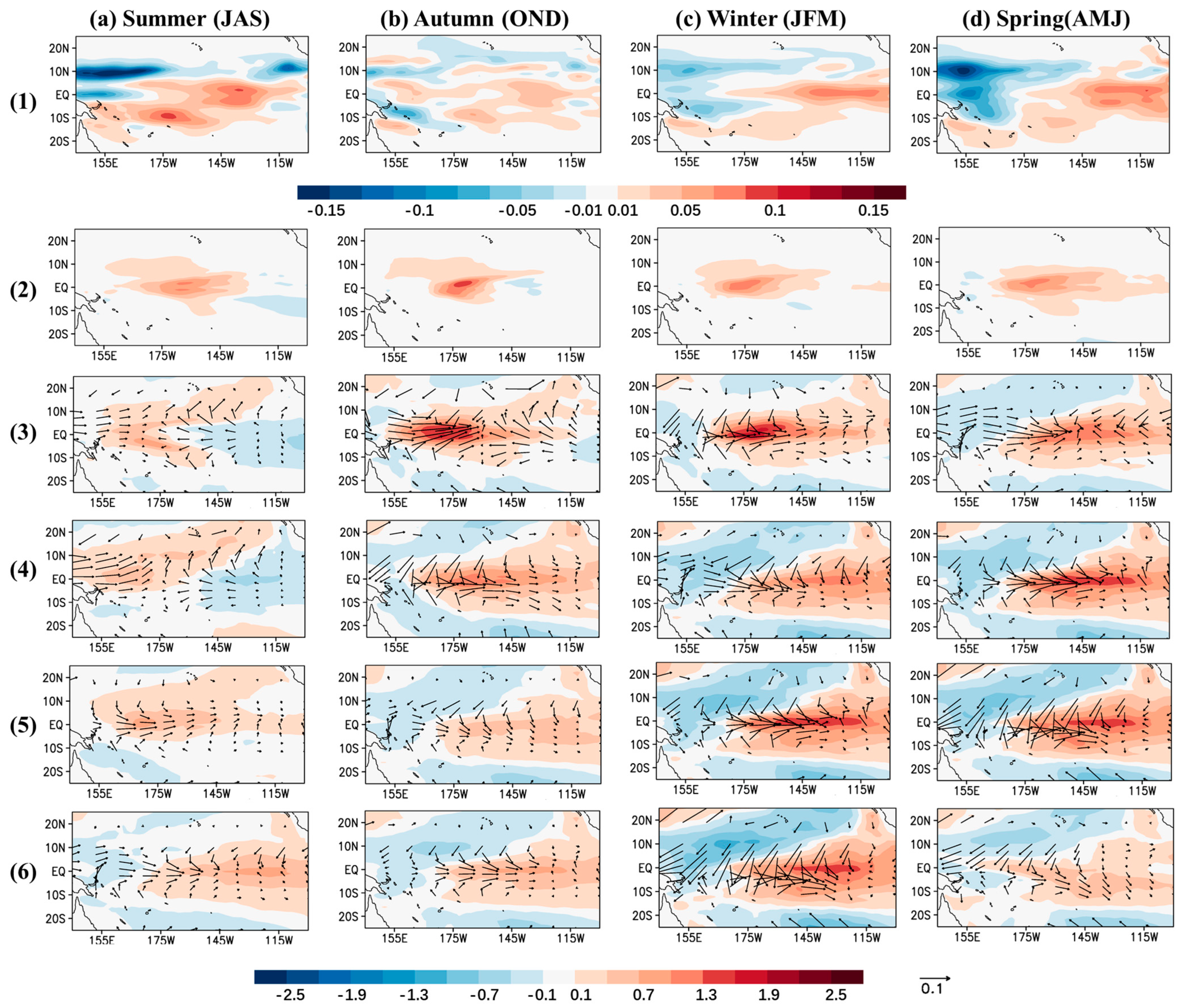
4.1. Patterns, Evolutions of OGEs and the Resulting SPB
4.1.1. SLA-OGEs
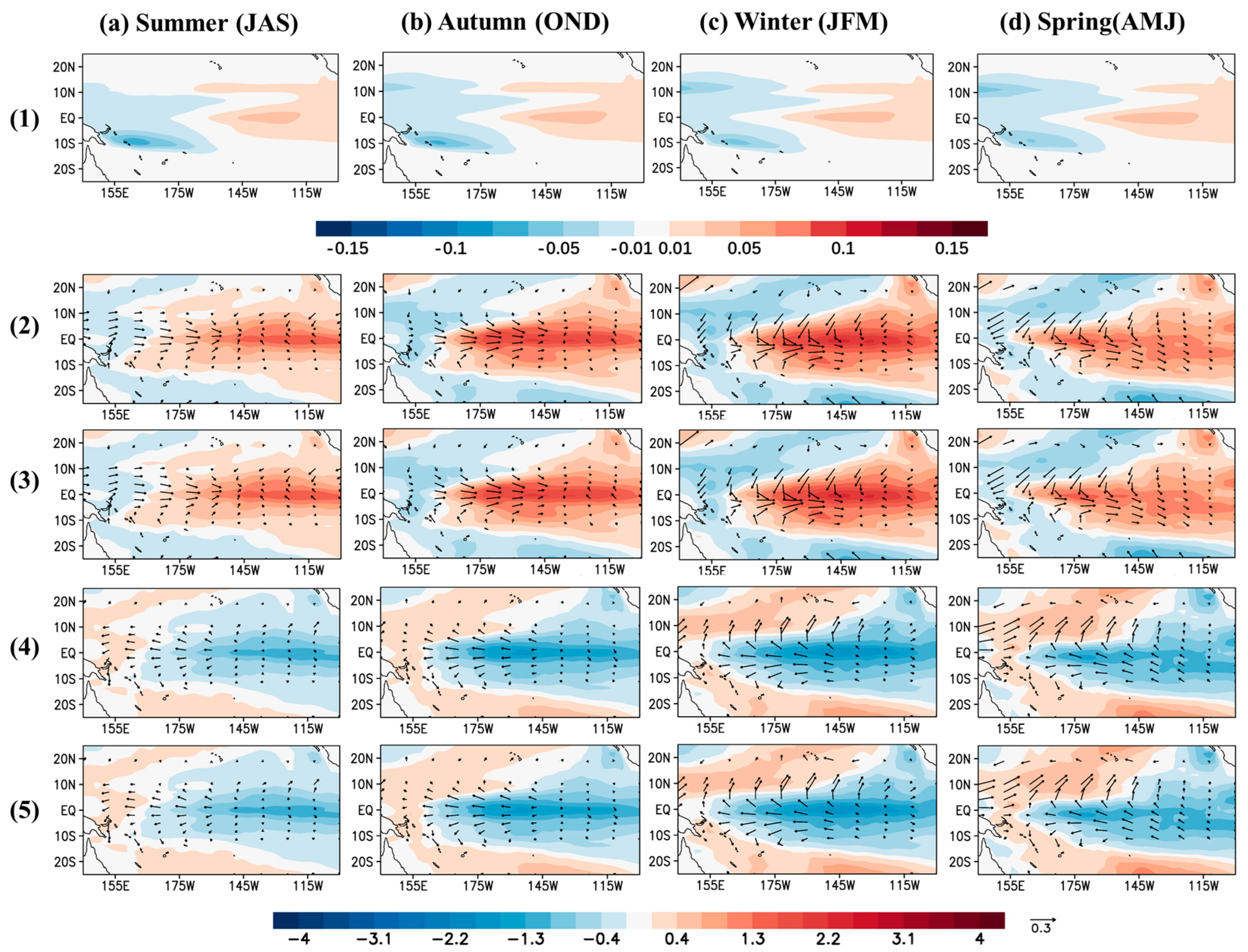
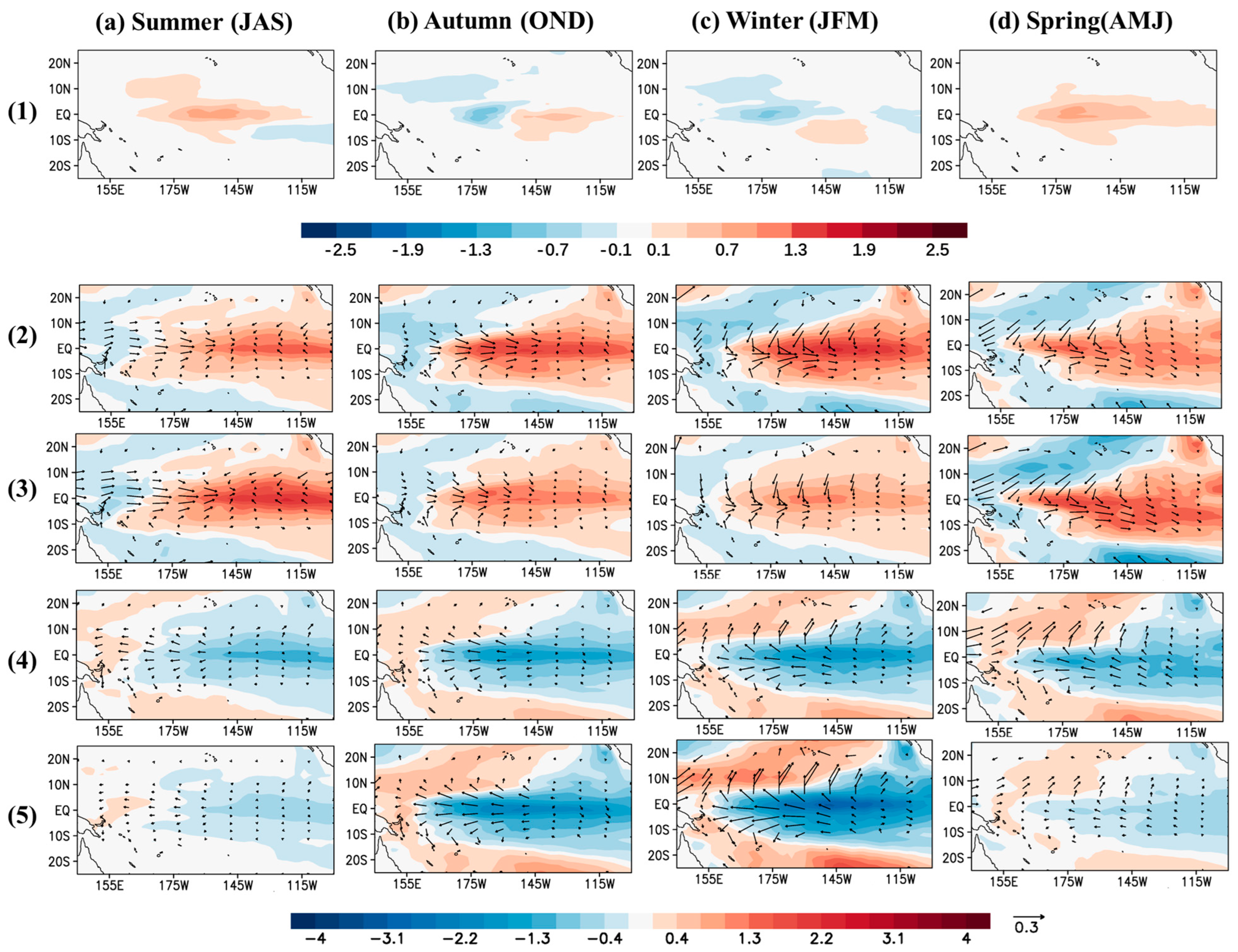
4.1.2. SSTA-OGEs
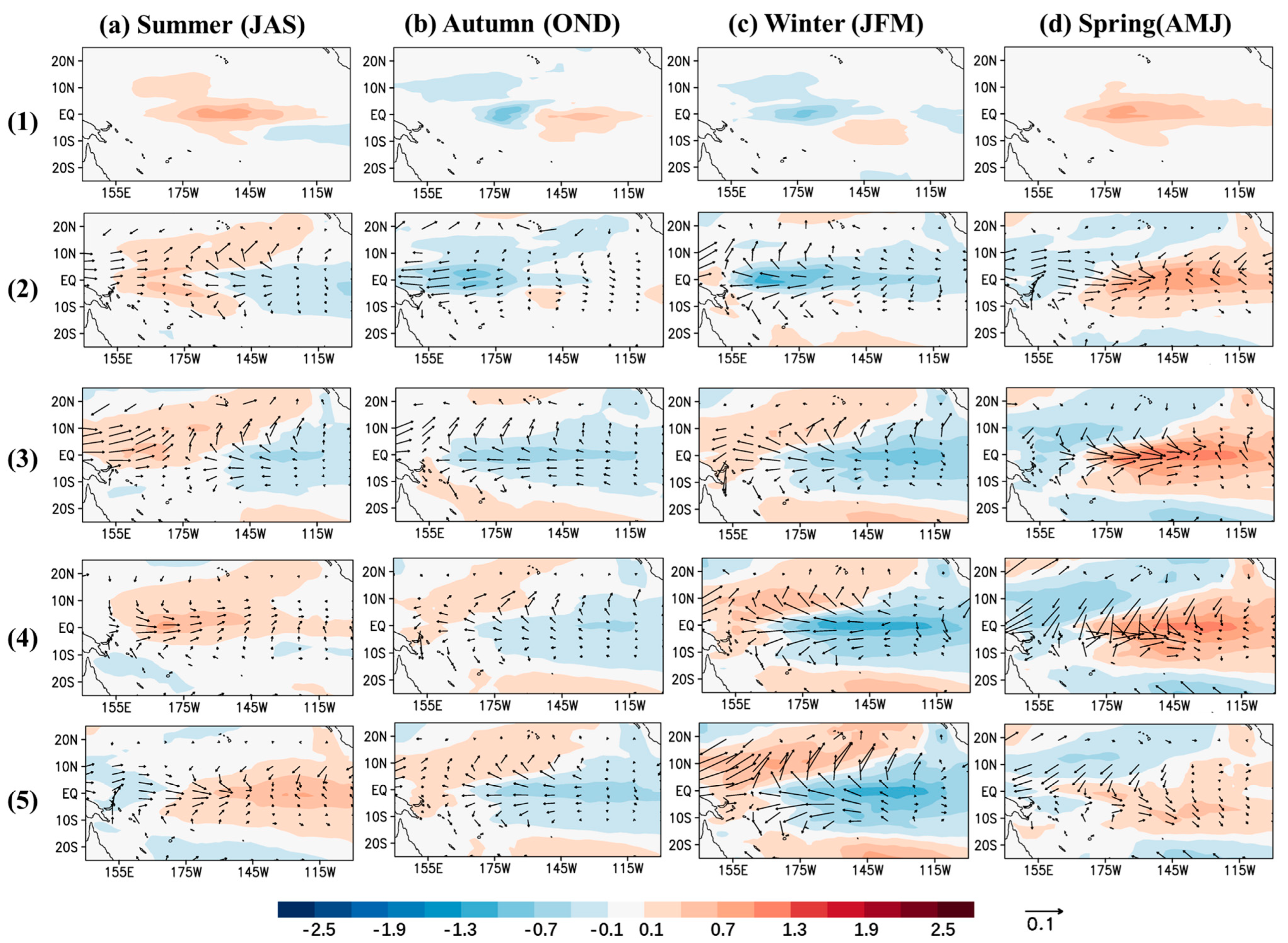
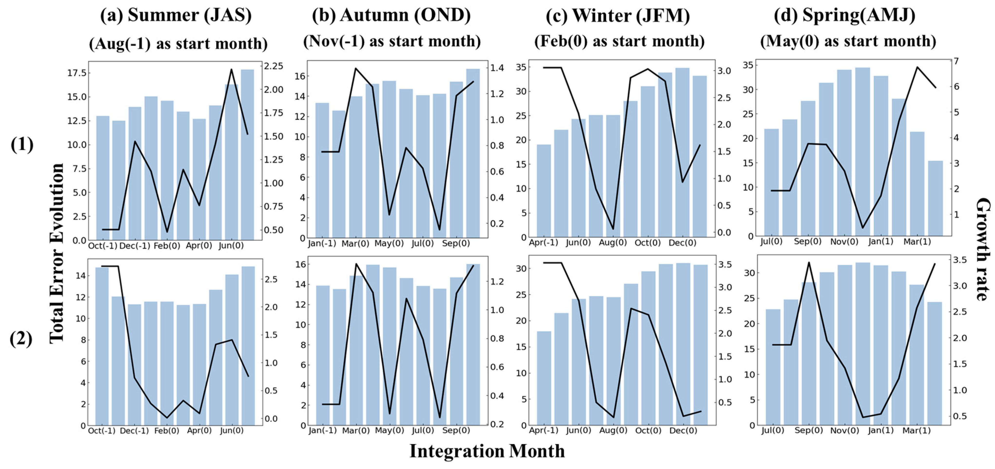
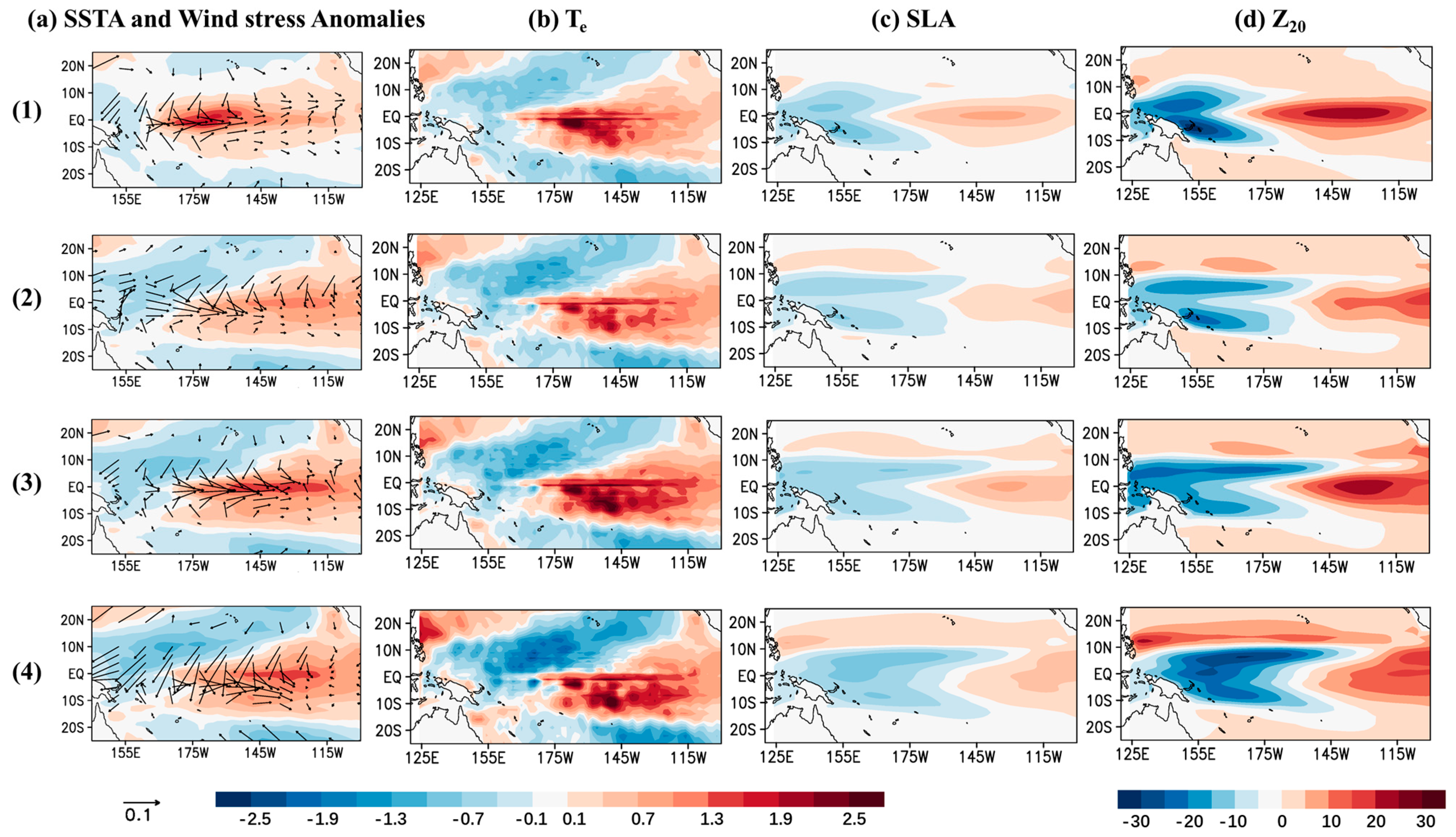
4.1.3. Joint-OGEs
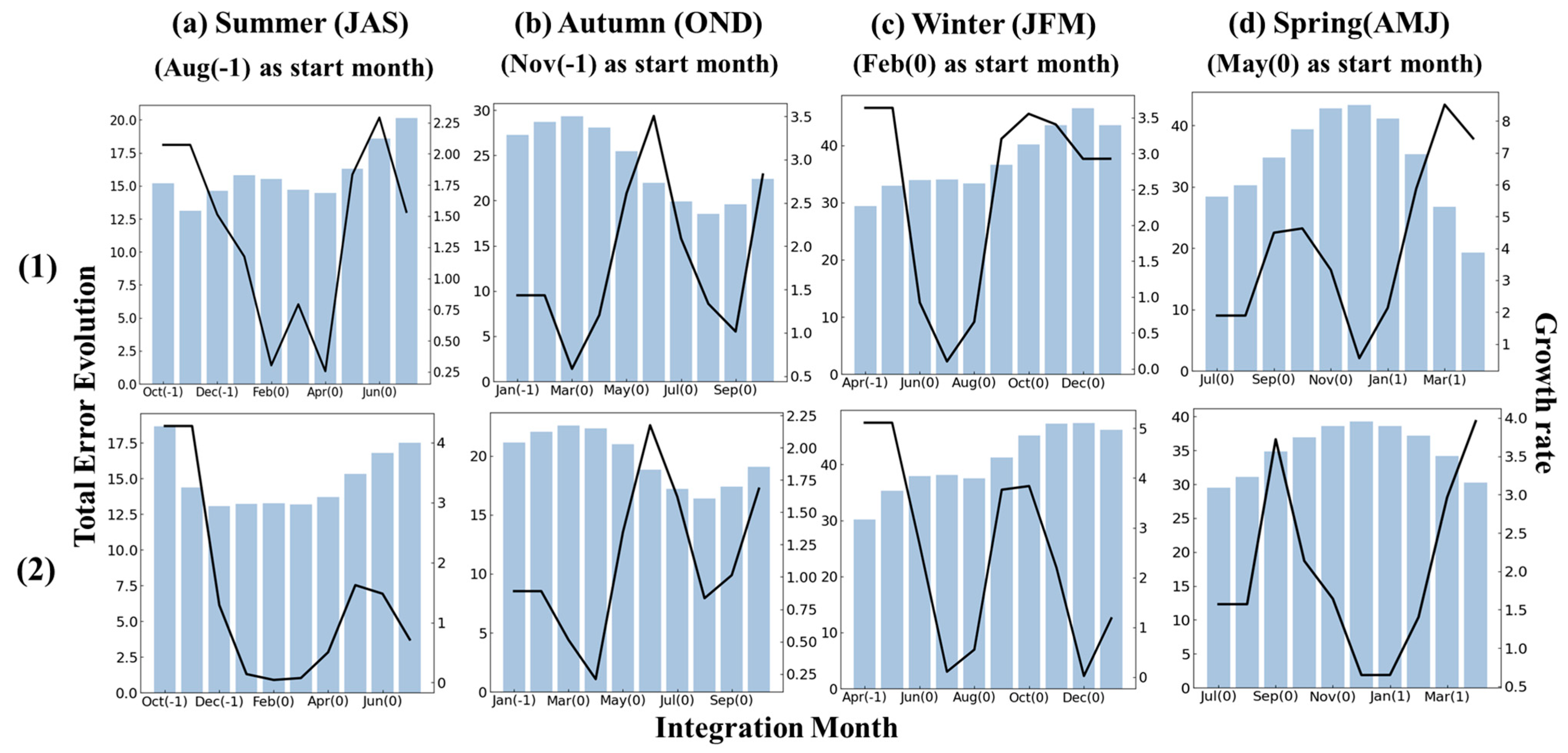
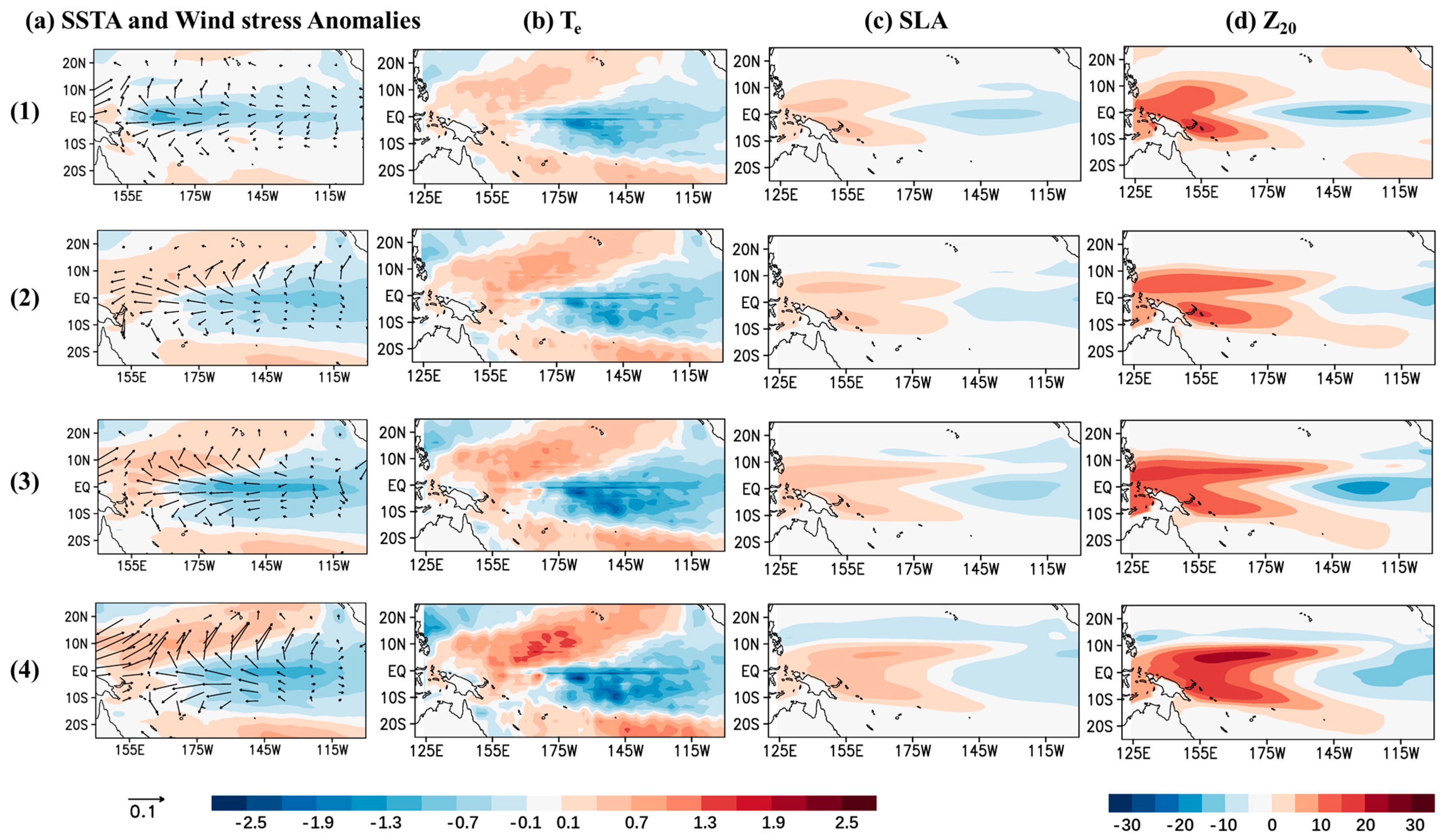
4.2. The Mechanism Analysis on OGE Evolutions and SPB
4.2.1. Dynamics Analysis on SLA-OGEs
4.2.2. Dynamics Analysis on SSTA-OGEs
4.2.3. Dynamics Analysis on Joint-OGEs
5. Target Observation Sensitive Area Identification
6. Conclusions
- We obtained a wide variety of OGE patterns. In addition to covering almost all the OGE modes obtained by previous studies, there are also extended OGE modes with more detailed information. Various OGEs have varying seasonal dependence and distinct effects on ENSO evolutions and the SPB.
- 2.
- By analyzing the mechanism of OGE evolutions and the SPB, we found that the principal physical processes involved in OGE evolutions also govern the SPB, which, induced by SSTA-OGEs, is mainly owing to Bjerknes feedback. For Joint-OGEs, the SPB is primarily due to the continuous heating between the upper ocean and the thermal diffusion in response to the discharge process.
- 3.
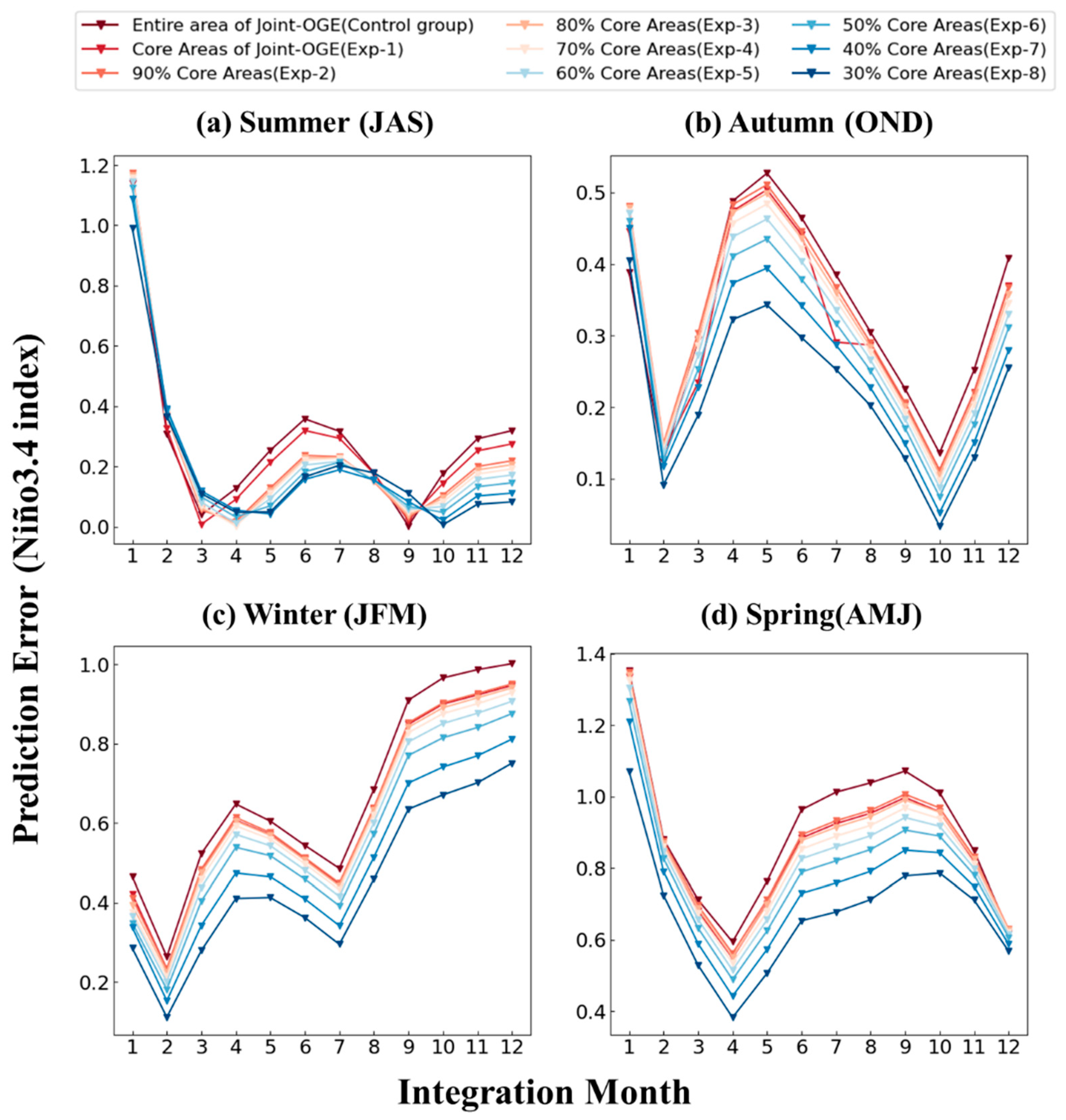
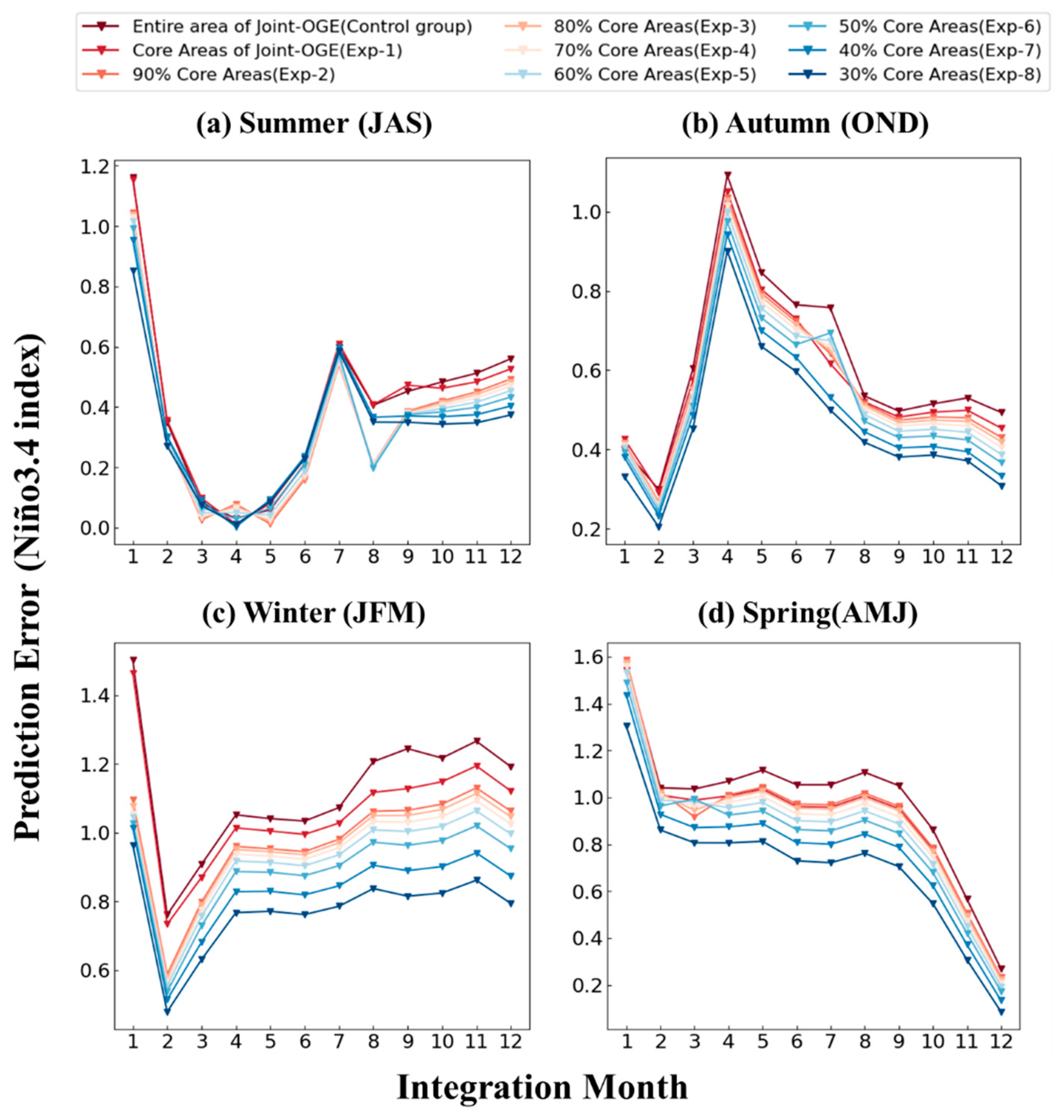
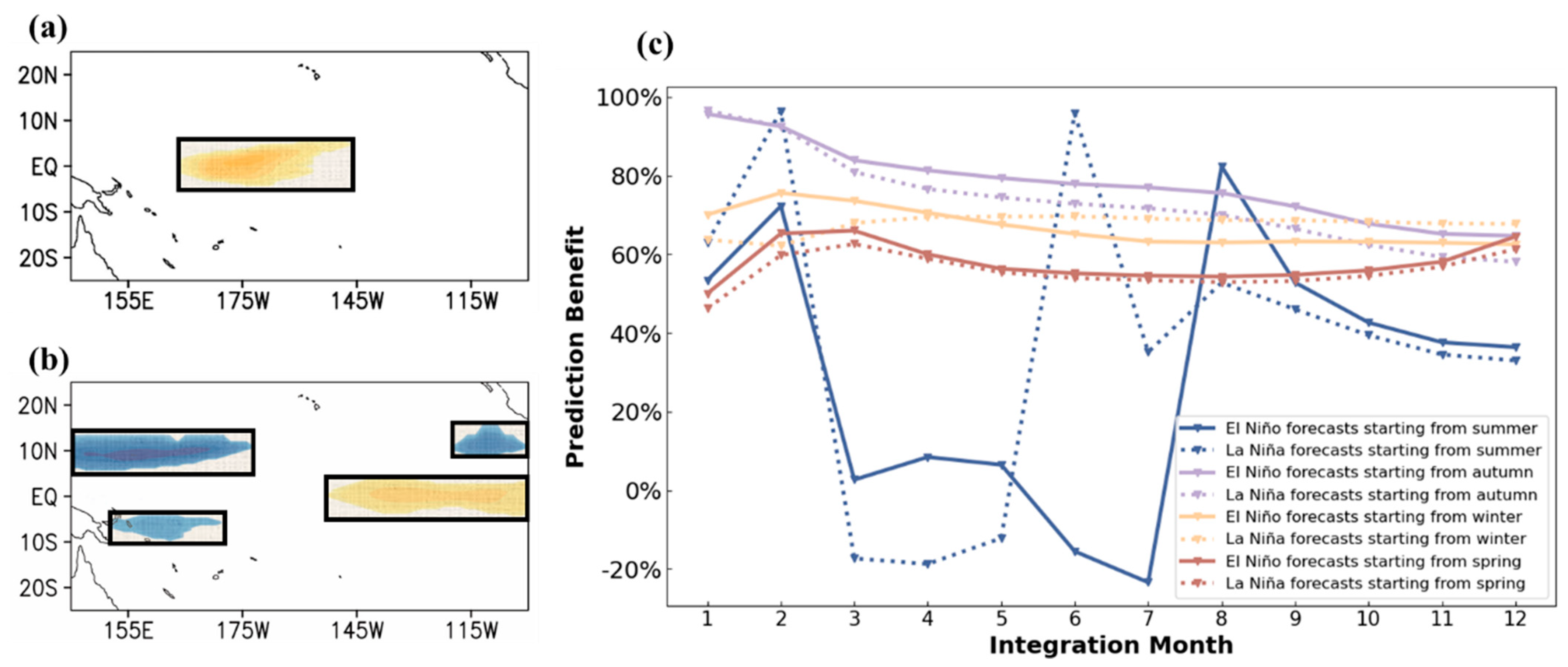
- Based on the Joint-OGE patterns, our observation scheme proposals include not only the most (economically) sensitive area schemes for each forecast starting from different seasons but also generic multivariate observation schemes. In detail, generic sensitive areas encompass the central-eastern equatorial Pacific and the western and north-eastern tropical Pacific boundary, where conducting intensive observation contributes to the ENSO prediction benefits, reaching 58.31% on average.
Author Contributions
Funding
Institutional Review Board Statement
Informed Consent Statement
Data Availability Statement
Conflicts of Interest
Appendix A

| No. | Term | Description |
|---|---|---|
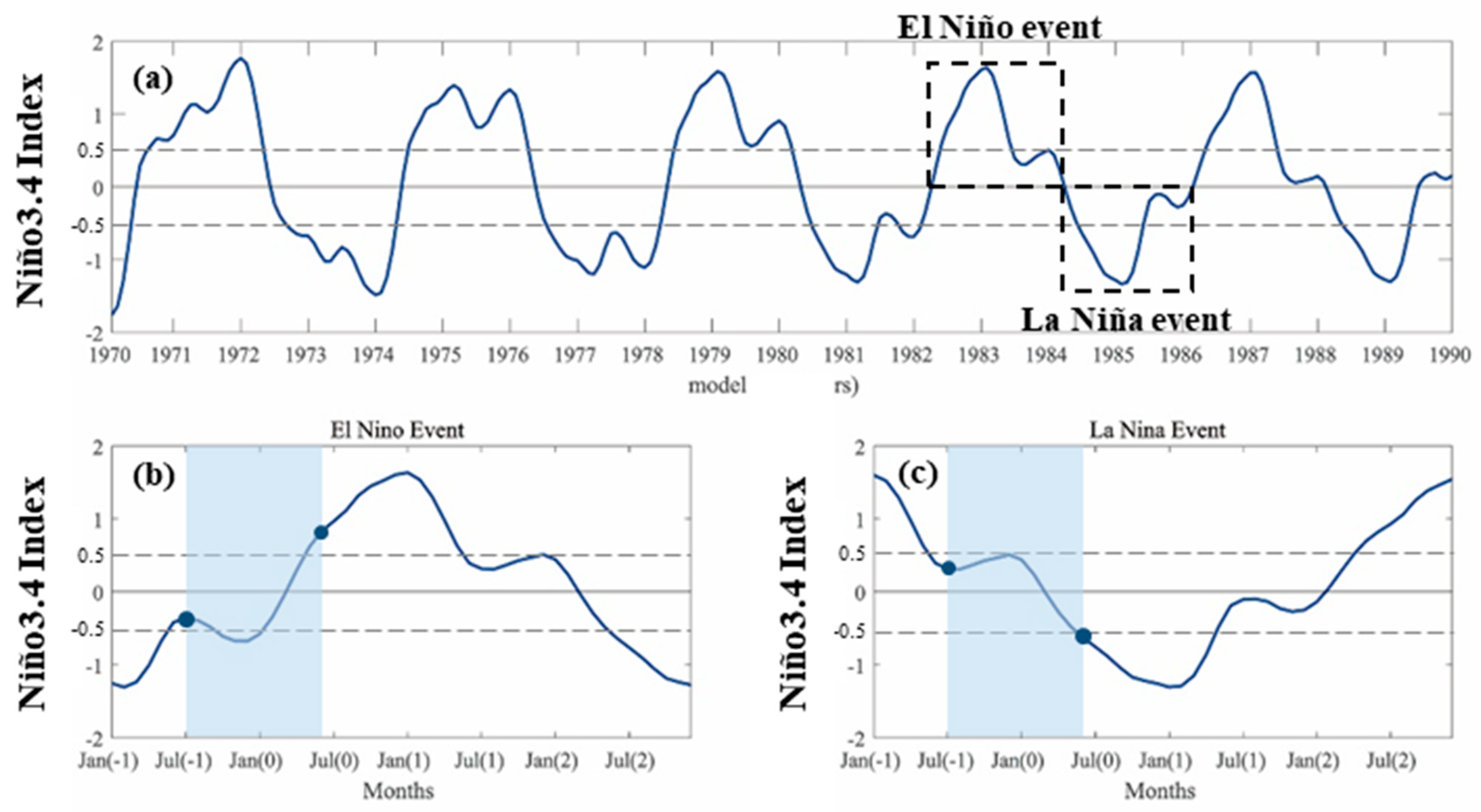
| 1 | ENSO data | The El Niño–Southern Oscillation |
| 2 | Niño3.4 index | mean of SST anomalies in the Niño 3.4 region (120° W–170° W, 5° N–5° S) |
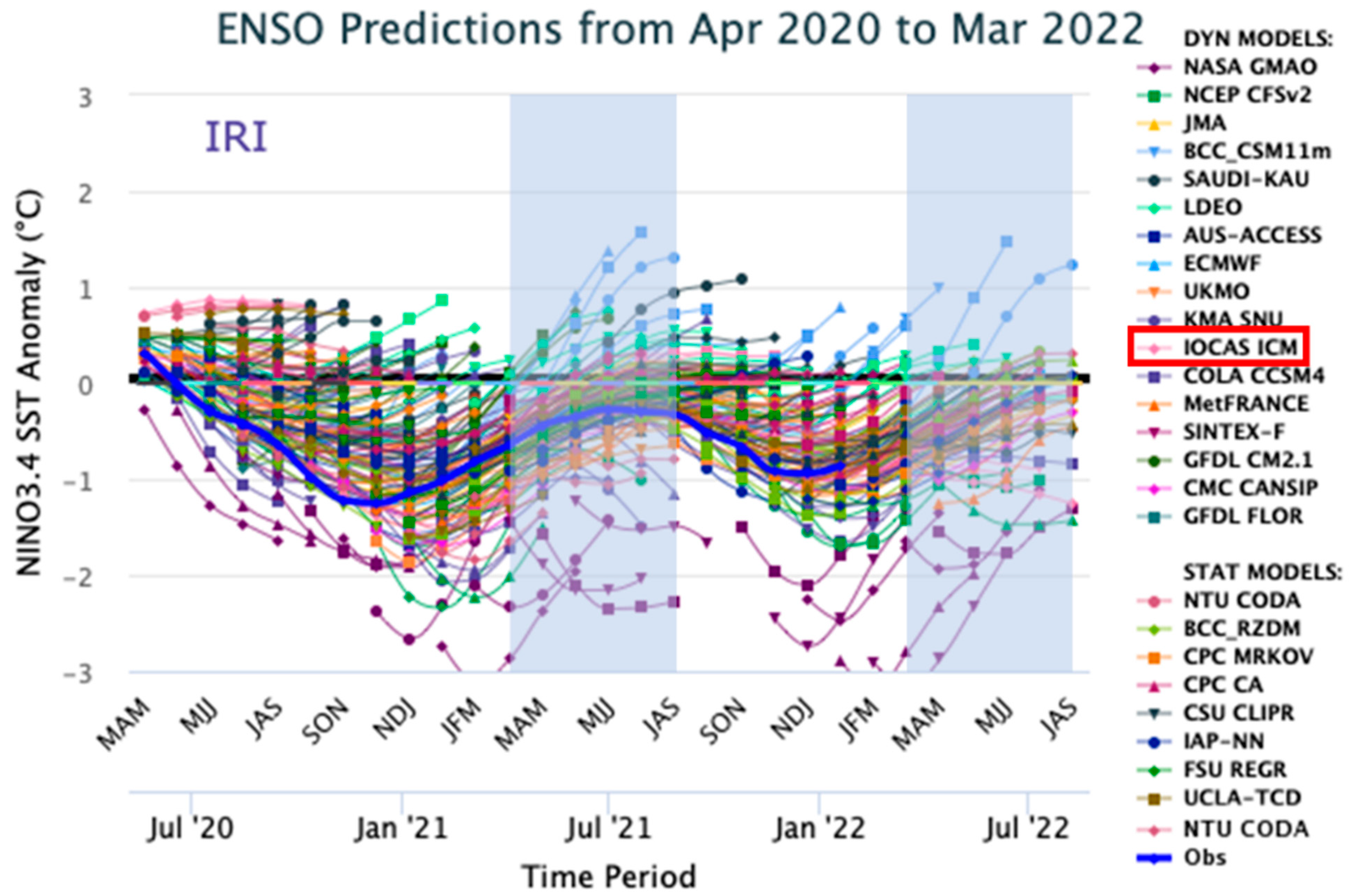
| 3 | IOCAS ICM | an intermediate coupled model developed at the Institute of Oceanology, Chinese Academy of Sciences |
| 4 | CNOP | conditional nonlinear optimal perturbation |
| 5 | PB | predictability barrier |
| 6 | SPB | spring predictability barrier |
| 7 | OGE | the optimal growth initial error |
| 8 | OPR | the optimal precursor |
| 9 | SSTA | sea surface temperature anomalies |
| 10 | SLA | sea level anomalies |
| 11 | THA | thermocline height anomalies |
| 12 | Te | the temperature of subsurface water entrained into the mixed layer |
| 13 | Z20 | 20 °C depth anomalies |
| 14 | SLA-OGE | the optimal growth initial error of SLA |
| 15 | SSTA-OGE | the optimal growth initial error of SSTA |
| 16 | Joint-OGE | the optimal growth initial error of SSTA and SLA |
| 17 | GD | gradient definition algorithm |
| 18 | ZC model | Zebiak–Cane model |
| 19 | MM5 | Mesoscale Model fifth Generation |
References
- Rasmusson, E.M.; Carpenter, T.H. Variations in tropical sea surface temperature and surface wind fields associated with the Southern Oscillation/El Niño. Mon. Weather Rev. 1982, 110, 354–384. [Google Scholar] [CrossRef]
- Philander, S.G.H. El Nino southern oscillation phenomena. Nature 1983, 302, 295–301. [Google Scholar] [CrossRef]
- Wyrtki, K. El Niño—The dynamic response of the equatorial Pacific Oceanto atmospheric forcing. J. Phys. Oceanogr. 1975, 5, 572–584. [Google Scholar] [CrossRef]
- Chen, D.; Cane, M.A.; Kaplan, A.; Zebiak, S.E.; Huang, D. Predictability of El Niño over the past 148 years. Nature 2004, 428, 733–736. [Google Scholar] [CrossRef]
- Beobide-Arsuaga, G.; Bayr, T.; Reintges, A.; Latif, M. Uncertainty of ENSO-amplitude projections in CMIP5 and CMIP6 models. Clim. Dyn. 2021, 56, 3875–3888. [Google Scholar] [CrossRef]
- Available online: https://iri.columbia.edu/our-expertise/climate/forecasts/enso/current/ (accessed on 20 October 2022).
- Fang, X.; Xie, R. A brief review of ENSO theories and prediction. Sci. China Earth Sci. 2020, 63, 476–491. [Google Scholar] [CrossRef]
- Liu, Z.; Jin, Y.; Rong, X. A theory for the seasonal predictability barrier: Threshold, timing, and intensity. J. Clim. 2019, 32, 423–443. [Google Scholar] [CrossRef]
- Zhang, R.H.; Zebiak, S.E.; Kleeman, R.; Keenlyside, N. A new intermediate coupled model for El Niño simulation and prediction. Geophys. Res. Lett. 2003, 30. [Google Scholar] [CrossRef]
- Zhang, R.H.; Gao, C. The IOCAS intermediate coupled model (IOCAS ICM) and its real-time predictions of the 2015–2016 El Niño event. Sci. Bull. 2016, 61, 1061–1070. [Google Scholar] [CrossRef]
- Zhang, R.H.; Tao, L.J.; Gao, C. An improved simulation of the 2015 El Niño event by optimally correcting the initial conditions and model parameters in an intermediate coupled model. Clim. Dyn. 2018, 51, 269–282. [Google Scholar] [CrossRef]
- Gao, C.; Chen, M.; Zhou, L.; Feng, L.; Zhang, R.H. The 2020–2021 prolonged La Niña evolution in the tropical Pacific. Sci. China Earth Sci. 2022, 65, 2248–2266. [Google Scholar] [CrossRef]
- Zhang, R.H.; Gao, C.; Feng, L. Recent ENSO evolution and its real-time prediction challenges. Natl. Sci. Rev. 2022, 9, nwac052. [Google Scholar] [CrossRef] [PubMed]
- Tao, L.J.; Zhang, R.H.; Gao, C. Initial error-induced optimal perturbations in ENSO predictions, as derived from an intermediate coupled model. Adv. Atmos. Sci. 2017, 34, 791–803. [Google Scholar] [CrossRef]
- Chen, H.; Wang, Q.; Zhang, R.H. Sensitivity of El Niño diversity prediction to parameters in an intermediate coupled model. Clim. Dyn. 2023, 1–18. [Google Scholar] [CrossRef]
- Tao, L.J.; Gao, C.; Zhang, R.H. ENSO predictions in an intermediate coupled model influenced by removing initial condition errors in sensitive areas: A target observation perspective. Adv. Atmos. Sci. 2018, 35, 853–867. [Google Scholar] [CrossRef]
- Tian, B.; Ren, H.L. Diagnosing SST Error Growth during ENSO Developing Phase in the BCC_CSM1.1(m) Prediction System. Adv. Atmos. Sci. 2022, 39, 427–442. [Google Scholar] [CrossRef]
- Lee, J.; Planton, Y.Y.; Gleckler, P.J.; Sperber, K.R.; Guilyardi, E.; Wittenberg, A.T.; McPhaden, M.J.; Pallotta, G. Robust evaluation of ENSO in climate models: How many ensemble members are needed? Geophys. Res. Lett. 2021, 48, e2021GL095041. [Google Scholar] [CrossRef]
- Zhou, Q.; Chen, L.; Duan, W.; Wang, X.; Zu, Z.; Li, X.; Zhang, S.; Zhang, Y. Using conditional nonlinear optimal perturbation to generate initial perturbations in ENSO ensemble forecasts. Weather Forecast. 2021, 36, 2101–2111. [Google Scholar] [CrossRef]
- L’Heureux, M.L.; Levine, A.F.; Newman, M.; Ganter, C.; Luo, J.J.; Tippett, M.K.; Stockdale, T.N. ENSO prediction. El Niño South. Oscil. A Chang. Clim. 2020, 227–246. [Google Scholar]
- Hu, J.; Duan, W.; Zhou, Q. Season-dependent predictability and error growth dynamics for La Niña predictions. Clim. Dyn. 2019, 53, 1063–1076. [Google Scholar] [CrossRef]
- Duan, W.; Liu, X.; Zhu, K.; Mu, M. Exploring the initial errors that cause a significant “spring predictability barrier” for El Niño events. J. Geophys. Res. Ocean. 2009, 114. [Google Scholar] [CrossRef]
- Mu, M.; Zhou, F.; Wang, H. A method for identifying the sensitive areas in targeted observations for tropical cyclone prediction: Conditional nonlinear optimal perturbation. Mon. Weather Rev. 2009, 137, 1623–1639. [Google Scholar] [CrossRef]
- Mu, B.; Cui, Y.; Yuan, S.; Qin, B. Simulation, precursor analysis and targeted observation sensitive area identification for two types of ENSO using ENSO-MC v1.0. Geosci. Model Dev. 2022, 15, 4105–4127. [Google Scholar] [CrossRef]
- Zhang, J.; Hu, S.; Duan, W. On the sensitive areas for targeted observations in ENSO forecasting. Atmos. Ocean. Sci. Lett. 2021, 14, 100054. [Google Scholar] [CrossRef]
- Mu, M.; Duan, W.S.; Wang, B. Conditional nonlinear optimal perturbation and its applications. Nonlinear Process. Geophys. 2003, 10, 493–501. [Google Scholar] [CrossRef]
- Mu, M.; Yu, Y.; Xu, H.; Gong, T. Similarities between optimal precursors for ENSO events and optimally growing initial errors in El Niño predictions. Theor. Appl. Climatol. 2014, 115, 461–469. [Google Scholar] [CrossRef]
- Xu, H.; Chen, L.; Duan, W. Optimally growing initial errors of El Niño events in the CESM. Clim. Dyn. 2021, 56, 3797–3815. [Google Scholar] [CrossRef]
- Yang, Z.; Fang, X.; Mu, M. Optimal Precursors for Central Pacific El Niño Events in GFDL CM2p1. J. Clim. 2023, 1–30. [Google Scholar] [CrossRef]
- Mu, B.; Ren, J.; Yuan, S.; Zhang, R.H.; Chen, L.; Gao, C. The optimal precursors for ENSO events depicted using the gradient-definition-based method in an intermediate coupled model. Adv. Atmos. Sci. 2019, 36, 1381–1392. [Google Scholar] [CrossRef]
- Bjerknes, J. Atmospheric teleconnections from the equatorial Pacific. Mon. Weather Rev. 1969, 97, 163–172. [Google Scholar] [CrossRef]
- Neelin, J.D.; Battisti, D.S.; Hirst, A.C.; Jin, F.F.; Wakata, Y.; Yamagata, T.; Zebiak, S.E. ENSO theory. J. Geophys. Res. Ocean. 1998, 103, 14261–14290. [Google Scholar] [CrossRef]
- Zelle, H.; Appeldoorn, G.; Burgers, G.; van Oldenborgh, G.J. The relationship between sea surface temperature and thermocline depth in the eastern equatorial Pacific. J. Phys. Oceanogr. 2004, 34, 643–655. [Google Scholar] [CrossRef]
- Meinen, C.S.; McPhaden, M.J. Observations of warm water volume changes in the equatorial Pacific and their relationship to El Niño and La Niña. J. Clim. 2000, 13, 3551–3559. [Google Scholar] [CrossRef]
- Keenlyside, N.; Kleeman, R. Annual cycle of equatorial zonal currents in the Pacific. J. Geophys. Res. Ocean. 2002, 107, 8-1–8-13. [Google Scholar] [CrossRef]
- Mu, B.; Ren, J.; Yuan, S. An efficient approach based on the gradient definition for solving conditional nonlinear optimal perturbation. Math. Probl. Eng. 2017, 2017, 3208431. [Google Scholar] [CrossRef]
- Mu, B.; Ren, J.; Yuan, S.; Zhou, F. Identifying typhoon targeted observations sensitive areas using the gradient definition based method. Asia-Pac. J. Atmos. Sci. 2019, 55, 195–207. [Google Scholar] [CrossRef]
- Li, X.; Hu, Z.Z.; Zhao, S.; Ding, R.; Zhang, B. On the asymmetry of the tropical Pacific thermocline fluctuation associated with ENSO recharge and discharge. Geophys. Res. Lett. 2022, 49, e2022GL099242. [Google Scholar] [CrossRef]
- O’Kane, T.J.; Squire, D.T.; Sandery, P.A.; Kitsios, V.; Matear, R.J.; Moore, T.S.; Risbey, J.S.; Watterson, I.G. Enhanced ENSO prediction via augmentation of multimodel ensembles with initial thermocline perturbations. J. Clim. 2020, 33, 2281–2293. [Google Scholar] [CrossRef]
- Zhao, S.; Jin, F.F.; Long, X.; Cane, M.A. On the breakdown of ENSO’s relationship with thermocline depth in the central-equatorial Pacific. Geophys. Res. Lett. 2021, 48, e2020GL092335. [Google Scholar] [CrossRef]
- Zhao, Y.; Di Lorenzo, E. The impacts of extra-tropical ENSO precursors on tropical Pacific decadal-scale variability. Sci. Rep. 2020, 10, 3031. [Google Scholar] [CrossRef]
- Duan, W.; Hu, J. The initial errors that induce a significant “spring predictability barrier” for El Niño events and their implications for target observation: Results from an earth system model. Clim. Dyn. 2016, 46, 3599–3615. [Google Scholar] [CrossRef]
- Shin, S.I.; Sardeshmukh, P.D.; Newman, M.; Penland, C.; Alexander, M.A. Impact of annual cycle on ENSO variability and predictability. J. Clim. 2021, 34, 171–193. [Google Scholar] [CrossRef]
- Mu, M.; Xu, H.; Duan, W. A kind of initial errors related to “spring predictability barrier” for El Niño events in Zebiak-Cane model. Geophys. Res. Lett. 2007, 34. [Google Scholar] [CrossRef]
- Yu, Y.; Duan, W.; Xu, H.; Mu, M. Dynamics of nonlinear error growth and season-dependent predictability of El Niño events in the Zebiak–Cane model. Q. J. R. Meteorol. Soc. A J. Atmos. Sci. Appl. Meteorol. Phys. Oceanogr. 2009, 135, 2146–2160. [Google Scholar] [CrossRef]
- Duan, W.; Wei, C. The ‘spring predictability barrier’for ENSO predictions and its possible mechanism: Results from a fully coupled model. Int. J. Climatol. 2013, 33, 1280–1292. [Google Scholar] [CrossRef]
- Zheng, F.; Zhu, J. Coupled assimilation for an intermediated coupled ENSO prediction model. Ocean Dyn. 2010, 60, 1061–1073. [Google Scholar] [CrossRef]
- Geng, T.; Cai, W.; Wu, L.; Yang, Y. Atmospheric convection dominates genesis of ENSO asymmetry. Geophys. Res. Lett. 2019, 46, 8387–8396. [Google Scholar] [CrossRef]


| Parameters | Value | Meaning | ||
|---|---|---|---|---|
| SSTA | SLA | Joint | ||
| DoF | 48 | 48 | 72 | Dimension of the feature space |
| δ | 15 | 15 | 20 | The constraint of the initial perturbation |
| Maxit | 50 | The maximum iteration step of SPG2 | ||
| Lead time (T) | 12 months | The integrating time of ICM | ||
| Absolute Isoline (SSTA(°C)/SLA(m)) | ||||
|---|---|---|---|---|
| Summer | Autumn | Winter | Spring | |
| Control group | Entire areas of Joint-OGEs | |||
| Core area (Exp. 1) | 0.1/0.003 | |||
| 90% of core area (Exp. 2) | 0.125/0.0332 | 0.1185/0.03112 | 0.1109/0.03216 | 0.113/0.0333 |
| 80% of core area (Exp. 3) | 0.1487/0.0367 | 0.134/0.03275 | 0.1245/0.03485 | 0.127/0.0372 |
| 70% of core area (Exp. 4) | 0.1806/0.0403 | 0.156/0.03453 | 0.143/0.0376 | 0.142/0.0415 |
| 60% of core area (Exp. 5) | 0.2173/0.0459 | 0.1825/0.03678 | 0.1689/0.0408 | 0.1662/0.0479 |
| 50% of core area (Exp. 6) | 0.255/0.0521 | 0.216/0.03912 | 0.204/0.0438 | 0.2026/0.0548 |
| 40% of core area (Exp. 7) | 0.3055/0.05915 | 0.25/0.042 | 0.243/0.0474 | 0.25405/0.062 |
| 30% of core area (Exp. 8) | 0.4102/0.06928 | 0.36/0.04453 | 0.3235/0.0523 | 0.381/0.0708 |
Disclaimer/Publisher’s Note: The statements, opinions and data contained in all publications are solely those of the individual author(s) and contributor(s) and not of MDPI and/or the editor(s). MDPI and/or the editor(s) disclaim responsibility for any injury to people or property resulting from any ideas, methods, instructions or products referred to in the content. |
© 2023 by the authors. Licensee MDPI, Basel, Switzerland. This article is an open access article distributed under the terms and conditions of the Creative Commons Attribution (CC BY) license (https://creativecommons.org/licenses/by/4.0/).
Share and Cite
Mu, B.; Qin, X.; Yuan, S.; Qin, B. Error Evolutions and Analyses on Joint Effects of SST and SL via Intermediate Coupled Models and Conditional Nonlinear Optimal Perturbation Method. J. Mar. Sci. Eng. 2023, 11, 910. https://doi.org/10.3390/jmse11050910
Mu B, Qin X, Yuan S, Qin B. Error Evolutions and Analyses on Joint Effects of SST and SL via Intermediate Coupled Models and Conditional Nonlinear Optimal Perturbation Method. Journal of Marine Science and Engineering. 2023; 11(5):910. https://doi.org/10.3390/jmse11050910
Chicago/Turabian StyleMu, Bin, Xiaoyun Qin, Shijin Yuan, and Bo Qin. 2023. "Error Evolutions and Analyses on Joint Effects of SST and SL via Intermediate Coupled Models and Conditional Nonlinear Optimal Perturbation Method" Journal of Marine Science and Engineering 11, no. 5: 910. https://doi.org/10.3390/jmse11050910